Sudden expansion and domain-wall melting of strongly interacting bosons in two-dimensional optical lattices and on multileg ladders

Abstract

We numerically investigate the expansion of clouds of hard-core bosons in the two-dimensional square lattice using a matrix-product-state–based method. This nonequilibrium set-up is induced by quenching the trapping potential to zero and our work is specifically motivated by a recent experiment with interacting bosons in an optical lattice [Ronzheimer et al., Phys. Rev. Lett. 110, 205301 (2013)]. As the anisotropy of the amplitudes $J_{x}$ and $J_{y}$ for hopping in different spatial directions is varied from the one- to the two-dimensional case, we observe a crossover from a fast ballistic expansion in the one-dimensional limit $J_{x}\gg J_{y}$ to much slower dynamics in the isotropic two-dimensional limit $J_{x}=J_{y}$. We further study the dynamics on multi-leg ladders and long cylinders. For these geometries we compare the expansion of a cloud to the melting of a domain wall, which helps us to identify several different regimes of the expansion as a function of time. By studying the dependence of expansion velocities on both the anisotropy $J_{y}/J_{x}$ and the number of legs, we observe that the expansion on two-leg ladders, while similar to the two-dimensional case, is slower than on wider ladders. We provide a qualitative explanation for this observation based on an analysis of the rung spectrum.

I Introduction

Ultracold quantum gases are famous for the possibility of realizing many-body Hamiltonians such as the Hubbard model, the tunability of interaction strength, and, effectively, also dimensionality Bloch et al. (2008). This provides access to genuine one-dimensional (1D) and two-dimensional (2D) physics as well as to the crossover physics between these limiting cases. Moreover, time-dependent changes of various model parameters can be used to explore the nonequilibrium dynamics of many-body systems (see Langen et al. (2015a); Gogolin and Eisert (2015); Eisert et al. (2015) for recent reviews). Timely topics that are investigated in experiments include the relaxation and thermalization dynamics in quantum quenches Greiner et al. (2002); Kinoshita et al. (2006); Hofferberth et al. (2007); Trotzky et al. (2012); Gring et al. (2012); Cheneau et al. (2012); Pertot et al. (2014); Will et al. (2015); Braun et al. (2015); Langen et al. (2015b), the realization of metastable states Xia et al. (2014); Vidmar et al. (2015), and nonequilibrium mass transport Schneider et al. (2012); Reinhard et al. (2013); Ronzheimer et al. (2013) and spin transport Hild et al. (2014). Due to the availability of powerful analytical and numerical methods such as bosonization Giamarchi (2004), exact solutions for integrable systems Essler et al. (2005), or the density matrix renormalization group method White (1992); Schollwöck (2005, 2011), a direct comparison between theoretical and experimental results is often possible in the case of 1D systems Cheneau et al. (2012); Trotzky et al. (2012); Ronzheimer et al. (2013); Braun et al. (2015).

Strongly interacting many-body systems in two spatial dimensions, however, pose many of the open problems in condensed matter theory and many-body physics, concerning both equilibrium and nonequilibrium properties. The reason is related to the lack of reliable numerical approaches. Exact diagonalization, while supremely flexible, is inherently restricted to small system sizes Rigol et al. (2008). Nevertheless, smart constructions of truncated basis sets by selecting only states from subspaces that are relevant for a given time-evolution problem have given access to a number of 2D nonequilibrium problems (see, e.g., Mierzejewski et al. (2011); Bonca et al. (2012)). The truncation of equation of motions for operators provides an alternative approach Uhrig (2009), which has also been applied to quantum quench problems in the 2D Fermi-Hubbard model Hamerla and Uhrig (2014). Quantum Monte Carlo methods can be applied to systems in arbitrary dimensions including nonequilibrium problems (see, e.g., Goth and Assaad (2012); Carleo et al. (2012, 2014)), but suffer, for certain systems and parameter ranges, from the sign problem Gull et al. (2011). Dynamical mean-field methods become accurate in higher dimensions, yet do not necessarily yield quantitatively correct results in 2D Eckstein et al. (2010).

Regarding analytical approaches, we mention just a few examples, including solutions of the Boltzmann equation Schneider et al. (2012), flow equations Moeckel and Kehrein (2008), expansions in terms of the inverse coordination number Queisser et al. (2014), semiclassical approaches Lux et al. (2014); Lux and Rosch (2015), or time-dependent mean-field approaches Schützhold et al. (2006); Schiró and Fabrizio (2010, 2011) such as the time-dependent Gutzwiller ansatz (see, e.g., Jreissaty et al. (2011, 2013)). All these methods have provided valuable insights into aspects of the nonequilibrium dynamics in two (or three) dimensions, yet often involve approximations. Recently, the application of a nonequilibrium Green’s function approach to the dynamics in the sudden expansion in the 2D Fermi-Hubbard model has been explored Schlünzen et al. (2015).

Although there have been very impressive recent applications Yan et al. (2011); Depenbrock et al. (2012); Stoudenmire and White (2012) of the density-matrix renormalization group (DMRG) method White (1992) to 2D systems, the method, in general, faces a disadvantageous scaling with system size in 2D Stoudenmire and White (2012); Schollwöck (2005). Tensor-network approaches Maeshima et al. (2001); Verstraete and Cirac (2004); Jordan et al. (2008) that were specifically designed to capture 2D many-body wave functions are an exciting development, with promising results for the $t-J$ model Corboz et al. (2011). A relatively little-explored area of research is the time evolution of 2D many-body systems in quantum quench problems using DMRG-type algorithms Zaletel et al. (2015); Dorando et al. (2009); Haegeman et al. (2011); Lubasch et al. (2011); James and Konik (2015).

In this work, we present the application of a recent extension Zaletel et al. (2015) of 1D matrix-product state (MPS) algorithms Vidal (2004); Daley et al. ; White and Feiguin (2004) that is specifically tailored to deal with long-range interactions. Such long-range interactions arise by mapping even a short-range Hamiltonian on a 2D lattice to a 1D chain for the application of DMRG.

Recent experiments have started to study the nonequilibrium dynamics of interacting quantum gases in 2D lattices or in the 1D-to-2D crossover Schneider et al. (2012); Ronzheimer et al. (2013); Brown et al. (2015). Motivated by Refs. Ronzheimer et al. (2013); Vidmar et al. (2015), we study the sudden expansion of hard-core bosons which is the release of a trapped gas into a homogeneous optical lattice after quenching the trapping potential to zero. The results of Ref. Ronzheimer et al. (2013) show that strongly interacting bosons in 2D exhibit a much slower expansion than their 1D counterpart. In the latter case, the integrability of hard core bosons leads to a strictly ballistic and (for the specific initial conditions of Ref. Ronzheimer et al. (2013)) fast expansion that is indistinguishable from the one of noninteracting fermions and bosons. In the 2D case, it is believed that diffusive dynamics sets in and virtually inhibits the expansion in the high-density region, leading to a stable high-density core surrounded by ballistically expanding wings Ronzheimer et al. (2013), similar to the behavior of interacting fermions in 2D Schneider et al. (2012). The characteristic feature of these diffusivelike expansions in contrast to the ballistic case is the emergence of a spherically symmetric high-density core, while the ballistic expansion unveils the topology of the underlying reciprocal lattice.

In our work, we investigate this problem for both 2D clusters that can expand symmetrically in the $x$ and $y$ directions [see Fig. 1(a)] and wide cylinders and ladders [see Fig. 1(b)]. We use the ratio of hopping matrix elements $J_{x}$ and $J_{y}$ along the $x$ and $y$ directions as a parameter to study the 1D-to-2D crossover. For the 2D expansion in the isotropic case $J_{x}=J_{y}$, we clearly observe the emergence of a spherically symmetric core, while for small values of $J_{y}<J_{x}$ and on the accessible time scales, the expansion is essentially 1D-like. We further compute the expansion velocities derived from the time dependence of the radius as a function of $J_{y}/J_{x}$.

Since we are, in general, able to reach both longer times and larger particle numbers in the case of ladders than in 2D, we present an extensive analysis of multileg ladders and cylinders [i.e., ladders with periodic boundary conditions in the (narrow) $y$ direction] with $L_{y}=2,3,4$ legs [see the sketch in Fig. 1(b)]. From the analysis of the expansion in 1D systems Vidmar et al. (2015), we expect that the short-time dynamics is identical to the melting of so-called domain-wall states Antal et al. (1998); Gobert et al. (2005); Lancaster and Mitra (2010), in which half of the system is empty while the other half contains one particle per site in the initial state [see the sketch in Fig. 1(c)]. The domain-wall melting has been attracting considerable attention as a nonequilibrium problem in 1D spin-$\frac{1}{2}$ systems (see, e.g., Antal et al. (1998); Gobert et al. (2005); Lancaster and Mitra (2010); Caux and Mossel ; Santos and Mitra (2011); Sabetta and Misguich (2013); Halimeh et al. (2014); Alba and Heidrich-Meisner (2014)). Our results show that this similarity between the expansion of clusters and the domain-wall melting carries over to the transient dynamics on $L_{y}$-leg ladder systems, irrespective of boundary conditions.

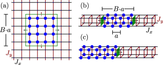
Figure 1: (Color online) Illustration of initial states and geometries: (a) central block for the 2D expansion; (b) central block of size $B\times L_{y}$; and (c) domain wall on a cylinder with $L_{y}=4$ legs.

A considerable portion of the discussion in both theoretical and experimental papers has focused on the question of whether there are signatures of diffusive dynamics in the sudden expansion in 2D, in the dimensional crossover Schneider et al. (2012); Ronzheimer et al. (2013), or on coupled chains Vidmar et al. (2013). The analysis of the expansion of fermions in the 2D square lattice starting from an initial state with two particles per site (i.e., a fermionic band insulator) suggests that diffusive dynamics is responsible for the slow expansion in the high-density regions Schneider et al. (2012). This is expected to carry over to the bosonic case, yet there only two-leg ladders have been thoroughly studied. In linear response, hard-core bosons on a two-leg ladder realize a textbook diffusive conductor at high temperatures Steinigeweg et al. (2014); Karrasch et al. (2015), thus suggesting that diffusion may also play a role in the sudden expansion Vidmar et al. (2013). Curiously, the expansion velocities measured numerically for hard-core bosons on a two-leg ladder exhibit a dependence on $J_{y}/J_{x}$ that resembles the experimental observations for the true 2D case Vidmar et al. (2013); Ronzheimer et al. (2013). Here we are able to provide a more refined picture. Our analysis unveils that the sudden expansion becomes faster by going from two-leg to three- or four-leg ladders. We trace this back to the existence of heavy excitations on the two-leg ladder that are defined on a rung of the ladder and are inherited from the $J_{x}\ll J_{y}$ limit, which cannot propagate in first-order tunneling processes in $J_{x}/J_{y}$. Conversely, the three- and four-leg ladders possess single-particle-like excitations, which we dub propagating modes, that have a sufficiently low mass to become propagating. This picture provides an intuitive understanding of the emergence of slow mass transport in the sudden expansion in the initial stages of the time evolution, complementary to the discussion of diffusive versus ballistic dynamics. The reasoning is similar to the role that doublons play for slowing down mass transport in the 1D Bose-Hubbard model Muth et al. (2012); Ronzheimer et al. (2013); Vidmar et al. (2013); Boschi et al. (2014); Sorg et al. (2014), which has also been emphasized in the case of the Fermi-Hubbard model Heidrich-Meisner et al. (2009); Kajala et al. (2011). Our results raise the question as to whether the expansion in both directions in 2D and the one-directional expansion on wide ladders and cylinders will result in the same dependence of expansion velocities on $J_{y}/J_{x}$ for large $L_{y}$. It appears that the ladders and cylinders, at least for small $L_{y}$, preserve some degree of one-dimensionality. A possible scenario is that the expansion velocities in the $x$ direction will depend nonmonotonically on $L_{y}$ for a fixed value of $J_{y}/J_{x}$ if ever they become identical to the behavior on the 2D systems. As a caution, we stress that long expansion times may be necessary to fully probe the effect of a 2D expansion at small $J_{y}\ll J_{x}$ since the bare time scale for charge dynamics in the $y$ direction is set by $1/J_{y}$, as pointed out in Schönmeier-Kromer and Pollet (2014).

Apart from the nonequilibrium mass transport of strongly interacting bosons, there are also predictions for the emergence of nonequilibrium condensates at finite quasimomenta in the sudden expansion in a 2D square lattice. These predictions are based on exact diagonalization for narrow stripes Hen and Rigol (2010), as well as on the time-dependent Gutzwiller method Jreissaty et al. (2011, 2013). The dynamical condensation phenomenon has first been discussed for 1D systems (where it actually is a quasicondensation Rigol and Muramatsu (2004)), where it was firmly established from exact numerical results Rigol and Muramatsu (2004, 2005a) and analytical solutions Lancaster and Mitra (2010) (see also Micheli et al. (2004); Daley et al. (2005); Rodriguez et al. (2006); Vidmar et al. (2013)) and has recently been observed in an experiment Vidmar et al. (2015). In the sudden expansion of hard-core bosons in 1D, the dynamical quasicondensation is a transient, yet long-lived phenomenon Rigol and Muramatsu (2004); Vidmar et al. (2013) as ultimately the quasimomentum distribution function of the physical particles approaches the one of the underlying noninteracting fermions via the dynamical fermionization mechanism Rigol and Muramatsu (2005b); Minguzzi and Gangardt (2005).

It is therefore an exciting question whether a true nonequilibrium condensate can be generated in 2D. Our results cannot fully clarify this point, yet we do observe a bunching of particles at certain nonzero momenta in the quasimomentum distribution after releasing the particles whenever propagating modes as discussed above are present. For the melting of domain walls, the occupation of most of these modes, at which a nonequilibrium condensation is allowed by energy conservation and at which a bunching occurs, saturates at long expansion times. The notable exception are certain modes on the $L_{y}=4$ cylinder. This behavior, i.e., the saturation is markedly different from the 1D case of hard-core bosons in the domain-wall melting, where the occupation continuously increases. The reason for this increase is that the semi-infinite, initially filled half of the system will indefinitely feed the quasicondensates Lancaster and Mitra (2010); Vidmar et al. (2015). As such an increase is a necessary condition for condensation, we interpret the saturation of occupations as an indication that either breaking the integrability of strictly 1D hard-core bosons or the larger phase space for scattering in 2D inhibits the dynamical condensation of expanding clouds. However, even in those cases on the ladder, in which we do not see a saturation, the increase is slower than the true 1D case, suggesting that coupling chains, in general, disfavors condensation. Yet a decisive analysis of this problem will require access to larger particle numbers and times in numerical simulations or future experiments. Note that multileg ladder systems can be readily realized with optical lattices, using either superlattices Fölling et al. (2007) or the more recent approach of using a synthetic lattice dimension Celi et al. (2014); Stuhl et al. (2015); Mancini et al. (2015). Using a synthetic lattice dimension Celi et al. (2014), it is in principle possible to obtain cylinders, i.e., periodic boundary conditions along the (narrow) $y$-direction.

The plan of this paper is the following. In Sec. II, we introduce the model and definitions. Section III provides a discussion and definitions for various measures of expansion velocities employed throughout our work, while Sec. IV provides details on our numerical method. We present our results for the 2D case in Sec. V, while the results for multileg ladders and cylinders are contained in Sec. VI. We conclude with a summary presented in Sec. VII, while details on the extraction of velocities and on the diagonalization of rung Hilbert spaces are contained in two appendixes.

II Model and initial conditions

We consider hard-core bosons on a square lattice and on multileg ladders. The Hamiltonian reads

$$H=-\sum_{i_{x},i_{y}}[J_{x}(\hat{a}^{\dagger}_{i_{x},i_{y}}\hat{a}^{\phantom{\dagger}}_{i_{x}+1,i_{y}}+h.c.)\,\\ +J_{y}(\hat{a}^{\dagger}_{i_{x},i_{y}}\hat{a}^{\phantom{\dagger}}_{i_{x},i_{y}+1}+h.c.)]\,.$$ (1)

Here $\hat{a}^{\dagger}_{i_{x},i_{y}}$ denotes the creation operator on site $\mathbf{i}=(i_{x},i_{y})$ and $J_{x}$($J_{y}$) are the hopping matrix elements in the $x$($y$) direction. We choose the hopping matrix element $J_{x}$ in the $x$ direction and the lattice constant $a$ as units and set $\hbar$ to unity; the ratio $J_{y}/J_{x}$ is dimensionless. Note that the Hamiltonian is equivalent to the spin-$\frac{1}{2}$ $XX$ model. In 1D ($J_{y}=0$), the Jordan-Wigner transformation maps the bosons to free fermions Cazalilla et al. (2011). $L_{x}$ and $L_{y}$ denote the number of sites in the $x$ and $y$ direction, respectively.

We consider different geometries, namely (i) a small square-shaped cluster of $L_{x}=L_{y}=12$ sites with open boundary conditions in both directions, (ii) ladders with $L_{x}=60$, $L_{y}\in\set{2,3,4}$ with open boundary conditions (OBCs) in both the $x$- and $y$-direction, and (iii) cylinders with $L_{x}=60$, $L_{y}\in\set{2,3,4}$ with periodic boundary conditions (PBCs) in the $y$ direction and OBCs in the $x$ direction. For two-leg ladders, the only difference between the Hamiltonian with OPC and PBC along the $y$ direction is thus a factor of two in the tunneling matrix element $J_{y}$. In praxis, we obtain the behavior with PBCs by just taking the OBCs data with $J_{y}\rightarrow J_{y}/2$.

For all simulations, we start the expansion from a product state,

$$|\psi_{0}\rangle=\prod_{{\bf i}\in\mathcal{B}}\hat{a}^{\dagger}_{i_{x},i_{y}}\ket{\rm vac},$$ (2)

in real space. To model the fully 2D expansion, we choose $\mathcal{B}$ to be a square-shaped block of $B\times B$ sites centered in the cluster; see Fig. 1(a). On cylinders and ladders, we study two different types of $\mathcal{B}$: (i) a block of $B\times L_{y}$ bosons, centered in the $x$ direction and filling all the sites in the $y$ direction as shown in Fig. 1(b), and (ii) a domain wall, where the left half of the lattice is occupied by a block of $L_{x}/2\times L_{y}$ bosons while the right half is empty; see Fig. 1(c).

III Definitions of expansion velocities

There are several possible ways of defining the spatial extension of an expanding cloud and thus also several different velocities.

III.1 Position of the fastest wave front

One can define the cloud size from its maximum extension, i.e., from the position of the (fastest) wave front. The velocity derived from this approach will typically simply be the fastest possible group velocity (provided the corresponding quasimomentum is occupied in the initial state). Thus, this velocity will not contain information about the slower-moving particles and any emergent slow and possibly diffusive dynamics in the core region. We do not study the wave front in this work.

III.2 Radial velocity

Theoretically, it is natural to define the radius $R$ as the square root of the second moment of the particle distribution $\langle n_{i}(t)\rangle$. Suppose we are interested in the expansion in $x$ direction: We average the density profile over the $y$ direction to calculate the radius

$$R_{x}^{2}(t)=\frac{1}{N}\sum_{i_{x},i_{y}}n_{i_{x},i_{y}}(t)(i_{x}a-i_{x}^{0}a)^{2},$$ (3)

where $i_{x}^{0}a$ is the center of mass in the $x$ direction and $N$ is the total number of bosons. An analogous expression is used to define $R_{y}^{2}$. To get rid of an initial constant part, we use $\tilde{R}_{\mu}^{2}(t)=R_{\mu}^{2}(t)-R_{\mu}^{2}(t=0)$ to define the radial velocity

$$v_{r,\mu}=\frac{\partial\tilde{R}_{\mu}(t)}{\partial t}\,$$ (4)

with $\mu=x,y$. The corresponding velocity has contributions from all occupied quasimomenta. It will ultimately be dominated by the fastest expanding particles, and for the sudden expansion, $R_{\mu}$ will be linear in time in the limit in which the gas has become dilute and effectively noninteracting.

The radial expansion velocity of 1D systems was studied for the Fermi-Hubbard model Langer et al. (2012), the Bose-Hubbard model Ronzheimer et al. (2013); Vidmar et al. (2013), and the Lieb-Liniger model Jukić et al. (2009). For Bethe-integrable 1D systems, it can be related to distributions of rapidities Mei et al. (2015). For a recent study of the radial velocity in the 2D Fermi-Hubbard model, see Schlünzen et al. (2015).

III.3 Core expansion velocity

In the related experiments with ultracold atoms Schneider et al. (2012); Ronzheimer et al. (2013), the focus was on the core expansion velocity that is derived from the time evolution of the half width at half maximum $r_{c}(t)$. The reason is that in these experiments, an average over many 1D or 2D systems is measured. Moreover, the core expansion velocity is primarily sensitive to the dynamics in the high-density core (but insensitive to the ballistic tails) and thus yields slightly different information. In case of multiple local maxima, the two outermost points are taken. Since in our simulations we have smaller particle numbers compared to the experiments Schneider et al. (2012); Ronzheimer et al. (2013), we use linear splines to interpolate the density profile between the lattice sites in order to get values for $r_{c}(t)$ to a better accuracy than just a single lattice constant. The core expansion velocity is defined as the time derivative

$$v_{c}=\frac{\partial r_{c}(t)}{\partial t}\,.$$ (5)

The full time dependence of $r_{c}$ and the extraction of $v_{c}$ is discussed in Appendix A.

IV Numerical Method

Although the Hamiltonian Eq. (1) itself is short ranged, long-range interactions arise by mapping the 2D lattice to a 1D DMRG chain. The presence of such long-range interactions renders most of the existing DMRG-based algorithms for the time evolution Vidal (2004); Daley et al. ; White and Feiguin (2004); Schollwöck (2011) inefficient because a direct Trotter decomposition of the exponential is not possible. In our work, we use a recently developed extension of an MPS-based time-dependent DMRG algorithm that is particularly suited for such systems Zaletel et al. (2015). The method is based on a local version of a Runge-Kutta step which can be efficiently represented by a matrix-product operator (MPO) Verstraete et al. (2004). The actual time evolution can then be performed using standard algorithms that apply an MPO to a given MPS Schollwöck (2011). An advantage of the method is that it can be easily implemented into an existing MPS based DMRG code and has a constant error per site.

For our simulations, we choose the DMRG chain to wind along the $y$ direction in order to keep the range of the interactions as small as possible (namely $L_{y}$). Sources of errors are the discretization in time and the discarded weight per truncation of the MPSs after each time step. The time steps are chosen small enough to make the error resulting from the second-order expansion negligible. We furthermore choose the truncation error at each step to be smaller than $10^{-10}$, which is sufficient to obtain all measured observables accurately. The growth of the entanglement entropy following the quench requires increasing the bond dimension $\chi$ with time. Conversely, since we restrict the number of states to $\chi\lesssim 2000$, we are naturally limited to a finite maximum time $t_{m}$ at which the truncation error becomes significant. Note that the bond dimension $\chi$ required for the simulations grows exponentially with time. Increasing the particle numbers and $L_{y}$ leads to a faster growth of the entanglement entropy and thus to a shorter maximal time $t_{m}$. However, we stress that we clearly reach longer times and larger systems than is accessible with exact diagonalization (i.e., pure state propagation using, e.g., Krylov subspace methods).

V Two-dimensional expansion

V.1 Density profiles

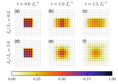
Figure 2: (Color online) Density profiles for the 2D expansion from a $4\times 4$ cluster with (a)–(c) $J_{y}/J_{x}=0.2$ and (d)–(f) $J_{y}/J_{x}=1.0$ at times $tJ_{x}=0.0,1.0,1.5$.

We first characterize the expansion by analyzing the time- and position-resolved density profile $n_{i_{x},i_{y}}(t)=\braket{\hat{n}_{i_{x},i_{y}}(t)}$, where $\hat{n}_{i_{x},i_{y}}=\hat{a}^{\dagger}_{i_{x},i_{y}}\hat{a}^{\phantom{\dagger}}_{i_{x},i_{y}}$ is the number operator. We present exemplary density profiles for three different times and and two anisotropies $J_{y}/J_{x}\in\set{0.2,1}$ in Fig. 2. For small $J_{y}/J_{x}=0.2$ [Figs. 2(a)–(c)], there is a fast expansion in the $x$ direction and nearly no expansion in the $y$ direction. This is expected since the bare timescale for the expansion in the $y$ direction set by $1/J_{y}$ is here much larger than the one in the $x$ direction Schönmeier-Kromer and Pollet (2014). On the other hand, for $J_{y}=J_{x}$, we find four “beams” of faster expanding particles going out along the diagonals. These beams are even more pronounced for initial states with smaller clusters of $2\times 2$ and $3\times 3$ bosons (not shown here).

The most important qualitative difference between the density profiles at $J_{y}/J_{x}=0.2$ and $J_{y}/J_{x}=1$ is the shape. In the former case, the profiles retain a rectangular form, reflecting the underlying reciprocal lattice and the different bare tunneling times in the $x$ versus the $y$ direction. For the isotropic case, the initial square shape of the cluster changes into a spherically symmetrical form in the high-density region. This observation is consistent with the experimental results of Ronzheimer et al. (2013).

V.2 Radial velocity

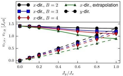
Figure 3: (Color online) Radial velocity $v_{r,x/y}$ in the $x$ direction (top three solid lines) and the $y$ direction (dashed lines) for the 2D expansion from $B\times B$ clusters. The small green triangles show the result of an extrapolation to $B=\infty$ using Eq. (6).

In order to compare the expansion for different values of $J_{y}/J_{x}$ more quantitatively, we extract certain integrated quantities from the profiles, which contain relevant information. One such quantity is the radial velocity $v_{r,x/y}$ derived from the reduced radius $\tilde{R}_{x/y}$ [see Eq. (3)]. Details on how we extract $v_{r}$ from the time-dependent reduced radius $\tilde{R}(t)$ can be found in Appendix A.

The radial velocities $v_{r,x}$ and $v_{r,y}$ for the 2D expansion are shown in Fig. 3. Unfortunately, our simulations for the 2D lattice are restricted to both very short times and small numbers of bosons with block sizes $B\in\set{2,3,4}$. For instance, for $4\times 4$ bosons we reach only times $t_{m}\approx 1.5\,J_{x}^{-1}$. The short times prevent us from a reliable extraction of the core expansion velocity, which would allow for a direct comparison to the experiment Schneider et al. (2012); Ronzheimer et al. (2013). The experimental results Ronzheimer et al. (2013) suggest that, for increasing $J_{y}$, the core expansion velocity in the $x$ direction decreases dramatically (see Fig. 8), which has been attributed to the breaking of integrability of 1D hard-core bosons Ronzheimer et al. (2013); Vidmar et al. (2013).

Our results for the radial velocity $v_{r}$ show that for the smallest block size $B=2$, tuning $J_{y}/J_{x}$ from 0 to 1 changes the velocity $v_{r,x}$ only gradually while the velocity in the $y$ direction scales almost linearly with $J_{y}$. A previous study of the expansion of two-leg ladders also indicated that the core expansion velocity exhibits a much stronger dependence on $J_{y}/J_{x}$ than the radial expansion velocity Vidmar et al. (2013). We suspect that this weak dependence may additionally result from the small number of bosons considered in our simulations: Increasing $J_{y}$ allows a hopping in the $y$ direction, which reduces the density and thus the effective interaction. In other words, tuning $J_{y}/J_{x}$ from 0 to 1 increases the effective surface of the initial block to include the upper and lower boundaries. From the surface, there is always a fraction of the bosons that escape and which effectively do not experience the hard-core interaction. This effect becomes more relevant for smaller boson numbers, where the bosons are almost immediately dilute, feel no effective interaction, and, thus, expand (nearly) ballistically in both directions. For larger block sizes $B=3,4$, the ratio of surface to bulk is smaller and, therefore, interaction effects become more relevant. Indeed, we find for $B=3,4$ that tuning $J_{y}/J_{x}$ from 0 to 1 leads to a significant reduction of $v_{r,x}$, most pronounced for $B=4$.

Even though we have access to only three values of $B$, it is noteworthy that for all values of $J_{y}/J_{x}$, $v_{r,x}(v_{r,y})$ decreases (increases) monotonically with $B$ and thus with total particle number. This tendency is compatible with the behavior of the experiments Ronzheimer et al. (2013) performed with much larger boson numbers, which motivates us to perform an extrapolation to $B=\infty$ despite the small number of bosons. We assume that the finite-size dependence is dominated by the surface effects of the initial boundary, which scales with $B$. Therefore, we extract the velocity for $B=\infty$ from a fit to the form

$$v_{r,x/y}(B)=v_{r,x/y}(B=\infty)+\frac{\mathrm{const}}{B}$$ (6)

at fixed $J_{y}/J_{x}$. The resulting values, which are indicated by the small green symbols in Fig. 3, should only be considered as rough estimates.

V.3 Momentum distribution function

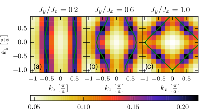
Figure 4: (Color online) Momentum distribution function $n_{k_{x},k_{y}}$ (dimensionless) for the 2D expanding cloud of $4\times 4$ bosons at time $t=1.5\,J_{x}^{-1}$. The solid green lines show the solutions to Eq. (8).

Figure 4 shows the momentum distribution function

$$n_{k_{x},k_{y}}=\frac{1}{L_{x}L_{y}}\sum_{i_{x},i_{y},j_{x},j_{y}}e^{-\mathrm{i}(k_{x}(i_{x}a-j_{x}a)+k_{y}(i_{y}a-j_{y}a))}\\ \times\braket{\hat{a}^{\dagger}_{i_{x},i_{y}}\hat{a}^{\phantom{\dagger}}_{j_{x},j_{y}}}$$ (7)

for the 2D expansion. For a purely 1D expansion ($J_{y}=0$), dynamical quasicondensation occurs at $k_{x}=\pm\frac{\pi}{2a}$ Rigol and Muramatsu (2004, 2005a); Vidmar et al. (2015). As discussed in Refs. Hen and Rigol (2010); Jreissaty et al. (2011), energy conservation restricts the (quasi)condensation to momenta at which the single-particle dispersion relation $\epsilon(k_{x},k_{y})$ vanishes since the initial state has zero energy, resulting in the emission of bosons with, on average, zero energy per particle. For a 2D system, this leads to

$$\epsilon(k_{x},k_{y}) =-2J_{x}\cos(k_{x}a)-2J_{y}\cos(k_{y}a)=0.$$ (8)

The solutions of this equation are indicated by the solid green lines in Fig. 4. We indeed observe an accumulation of particles at momenta compatible with Eq. (8). For $J_{y}/J_{x}=0.2$ [Fig. 4(a)], there is almost the same weight at any momentum $k_{y}$ compatible with Eq. (8). We suspect that this is a relict of the short time $t=1.5\,J_{x}^{-1}=0.3\,J_{y}^{-1}$ reached in the simulations: Up to this time there was almost no expansion in the $y$ direction; thus, we have roughly $\braket{\hat{a}^{\dagger}_{i_{x},i_{y}}\hat{a}^{\phantom{\dagger}}_{j_{x},j_{y}}}\approx\delta_{i_{y},j_{y}}$ such that $n_{k_{x},k_{y}}$ is initially independent of $k_{y}$. Nevertheless, closer inspection shows slightly more weight at compatible momenta with $k_{y}=\pm\frac{\pi}{2a}$ than at those with $k_{y}=0$ even for small $J_{y}$ [see Fig. 4(a)]. This becomes much more pronounced for $J_{y}=J_{x}$ [see Fig. 4(c)]. In this case, the strongest peaks are at $(k_{x},k_{y})=(\pm\frac{\pi}{2a},\pm\frac{\pi}{2a}),(\pm\frac{\pi}{2a},\mp\frac{\pi}{2a})$. These four points correspond to the maximum group velocities $v(k_{x},k_{y})=(2J_{x}a\sin(k_{x}a),2J_{y}a\sin(k_{y}a))$ and, in real space, manifest themselves via the four “beams” in the density profile shown in Fig. 2(f).

Our results do not serve to clarify whether there actually is a dynamical condensation at finite momenta in 2D or not since our initial clusters have too few particles in the bulk compared to their surface. The fast ballistic propagation of the particles melting away from the surface will only be suppressed once the majority of particles is in the bulk initially. If we attribute the outermost particles to the surface, this would require us to be able to simulate at least $7\times 7$ clusters. We believe that the accumulation at finite momenta seen in the quasimomentum distribution function is due to these fast particles melting away from the boundary during the first tunneling time. Moreover, we would need to be able to study the particle-number dependence of the height of the maxima in the quasimomentum distribution function or the decay of single-particle correlations over sufficiently long distances Rigol and Muramatsu (2004).

VI Cylinders and ladders

In contrast to the 2D lattice, the ratio of surface to bulk is much lower for cylinders and ladders, as we initialize the system uniformly in the $y$ direction. Moreover, if we tune $J_{y}$ from 0 to 1, the additional hopping in the $y$ direction does not lower the density (and with it the effective interaction), as it is the case for the fully 2D expansion. We thus expect a weaker dependence of the results on the number of bosons. Additionally, we can reach larger times than for the fully 2D expansion since the range of hopping terms after mapping to the DMRG chain is smaller. While we can reach times up to $t_{m}\approx 6\,J_{x}^{-1}$ for $L_{y}=2$, we are restricted to times up to $t_{m}\approx 4\,J_{x}^{-1}$ for $L_{y}=3$ and $t_{m}\approx 3\,J_{x}^{-1}$ for $L_{y}=4$.

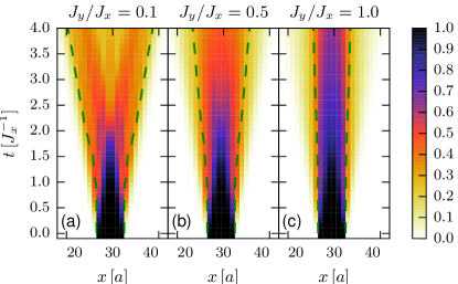
Figure 5: (Color online) Integrated density profiles $\frac{1}{L_{y}}\sum_{i_{y}}n_{i_{x},i_{y}}(t)$ (dimensionless) for the expansion from a $6\times 3$ cluster on a cylinder with $L_{y}=3$. The green dashed lines show the location of the half maximum on the left and right.

VI.1 Density profile

Figure 5 shows some typical results for the column density for the expansion of a block on a cylinder with $L_{y}=3$. We identify three different time regimes for the expansion of blocks, schematically depicted in Fig. 6. First, the evolution during the first tunneling time $t_{1}\propto 1/J_{x}$ is independent of $J_{y}$: Since we initialize our system uniformly in $y$ direction, in the initial longitudinal hopping, there cannot be any dependence on $J_{y}$ and a finite amount of time is required before correlations in the $y$ direction can build up.

Then, in a transient regime $0<t_{2}$ (where $t_{2}>t_{1}$), the melting of the block from either side is equivalent to the domain-wall melting Gobert et al. (2005); Vidmar et al. (2015) (compare the sketch in Fig. 1). From the two boundaries, two “light cones” emerge, consisting of particles outside and holes inside the block. Both particles and holes have a maximum speed of $v_{m}=2\,J_{x}a$. Consequently, the time $t_{2}:=B/4J_{x}$ is the earliest possible time at which the melting arrives at the center, such that the density drops below one on all sites. Thus, $t_{2}$ marks the point in time at which density profiles obtained from blocks start to differ quantitatively from those of domain walls, defining the third time regime. In the case of a ballistic expansion realized for $J_{y}\ll J_{x}$, the density in the center drops strongly at $t_{2}$ and we can clearly identify two outgoing “jets” as two separating maxima in the density profiles; see Fig. 5(a). To be clear, the expectation for the nature of mass transport in a nonintegrable model such as coupled systems of 1D hard-core bosons is diffusion, sustained by numerical studies Steinigeweg et al. (2014). However, in the sudden expansion, the whole cloud expands and it is conceivable that the expansion appears to be ballistic because the cloud becomes dilute too fast, resulting in mean-free paths being on the order of or larger than the cloud size at any time Vidmar et al. (2013).

Figure 6: Illustration of the time regimes for the expansion of blocks (see the text in Sec. VI.1 for details).

On the other hand, for larger $J_{y}$ the block in the center does not split at $t_{2}$, but a region with a high density (“core”) remains in the center. The high-density core is clearly established already at intermediate $J_{y}/J_{x}=0.5$, where it still expands slowly. For larger $J_{y}$, the spreading of this core is continuously suppressed.

VI.2 Integrated current

In order to investigate the different time regimes further, we consider the number of bosons $\Delta N(t)$ that at a time $t$ have left the block $\mathcal{B}$ where they were initialized. This is equivalent to the particle current $j^{x}_{i_{x}}=\mathrm{i}J_{x}\sum_{i_{y}}\langle\hat{a}^{\dagger}_{i_{x}+1,i_{y}}\hat{a}^{\phantom{\dagger}}_{i_{x},i_{y}}-\hat{a}^{\dagger}_{i_{x},i_{y}}\hat{a}^{\phantom{\dagger}}_{i_{x}+1,i_{y}}\rangle$ integrated over time and along the boundary $\partial\mathcal{B}$ of the block,

$$\Delta N(t)=\sum_{i\notin\mathcal{B}}n_{i_{x},i_{y}}(t)=\int_{0}^{t}{\rm d}s\,\left[j^{x}_{b_{r}}(s)-j^{x}_{b_{l}}(s)\right].$$ (9)

Here $b_{r}$ and $b_{l}$ denote the right and left indices $i_{x}$ of the boundary of the initially centered block $\mathcal{B}$. We compare $\Delta N$ for the expansion on a two-leg ladder starting from either central blocks or domain walls in Fig. 7(a). To this end we normalize $\Delta N$ by the boundary length $|\partial\mathcal{B}|$, which is simply $2L_{y}\,a$ for the central blocks and $L_{y}\,a$ for the domain walls.

For short times $t\lesssim 0.5\,J_{x}^{-1}$ (i.e., $t\lesssim t_{1}$, see the above), all curves in Fig. 7 are independent of $J_{y}$. For the quantity $\Delta N$, the first deviations between domain walls and cylinders do not occur at $t_{2}$ but at $2t_{2}=B/2J_{x}$, which is exactly the time the fastest holes need to travel once completely through the block: By definition, $\Delta N$ is not sensitive to the density inside the initial block. For the expansion of central blocks, particle conservation gives a strict bound $\Delta N/|\partial\mathcal{B}|\leq B/2a$, in which case all the bosons have left the initial block. These bounds (equal to $1.5\,a^{-1}$ and $3\,a^{-1}$ for $B=3$ and $B=6$, respectively) are approached in the long-time limit of the ballistic expansion for small $J_{y}/J_{x}=0.2$, which for $B=6$, however, happens beyond the times reached in our simulations. For the domain walls, $\Delta N$ is not bounded (as long as the melting does not reach the boundary of the system) and grows for small $J_{y}/J_{x}$ as $\Delta N\propto t$ linearly in time, which, via Eq. (9), corresponds to a nondecaying current $j^{x}$. On the other hand, $\Delta N$ gets almost constant for large $J_{y}/J_{x}$ for both the domain walls and the blocks. This indicates that the expansion is strongly suppressed on the two-leg ladder, with a high-density core remaining in the center. We speculate that the regime in which $\Delta N$ increases only very slowly is indicative of diffusive dynamics, by similarity with Schneider et al. (2012).

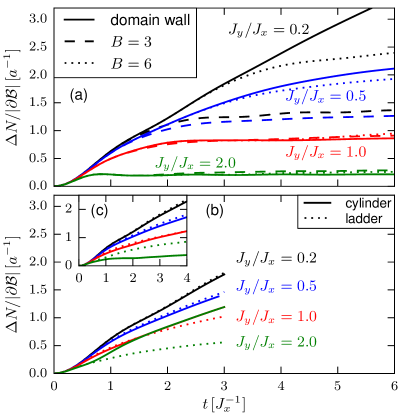
Figure 7: (Color online) Comparison of $\Delta N/|\partial\mathcal{B}|$ (a) on a two-leg ladder for the expansion from central blocks (dashed/dotted lines, $B\times 2$ bosons) versus the melting of a domain wall (solid lines). The lower panels compare domain walls on ladders (dashed lines) to domain walls on cylinders (solid lines) for (b) $L_{y}=4$ and (c) $L_{y}=3$. The curves for the $L_{y}=4$ cylinder in (b) with $J_{y}/J_{x}=1,2$ are nearly on top of each other for $t\gtrsim 1.5\,J_{x}^{-1}$.

VI.3 Propagating modes: Limit of large $J_{y}\gg J_{x}$

In order to qualitatively understand the suppression of the expansion for certain geometries and specific values of $L_{y}$, it is very instructive to consider the limit of large $J_{y}\gg J_{x}$. We discuss this limit in more detail in Appendix B, while here, we provide only the general idea and discuss the results. The Hamiltonian Eq. (1) can be split up into the hopping on rungs (we denote sites with the same index $i_{x}$ as a “rung” for both ladders and cylinders), denoted by $H^{y}$ proportional to $J_{y}$, and the hopping terms in the $x$ direction proportional to $J_{x}$, collected in $H^{x}$. Our analysis is based on a diagonalization of $H^{y}$, which is a block-diagonal product of terms operating on single rungs. We view the eigenstates of single rungs as “modes,” which can be delocalized by $H^{x}$. Since a coherent movement of multiple bosons is a higher-order process of $H^{x}$ and thus generally suppressed for large $J_{y}/J_{x}$, we focus on modes with a single particle on a rung. We then look for modes which are candidates for a propagation at finite $k_{x}$. Importantly, the kinetic energy $E_{x}\propto J_{x}$ cannot compensate for a finite $E_{y}\propto J_{y}$ for $J_{y}\gg J_{x}$. Since we initialize the system in states with zero total energy, energy conservation allows only modes with $E_{y}=0$ to contribute to the expansion in first-order processes in $J_{x}/J_{y}$ in time. In general, one could also imagine to create pairs of two separate bosons with exactly opposite $E_{y}$, summing up to 0. Yet $H^{x}$ cannot create such pairs (see Appendix B for details).

For smaller $J_{y}$, the scaling argument of the energy conservation does not hold and additional modes (beginning with those of small energy $E_{y}$) can be used for the propagation in the the $x$ direction; ultimately, for $J_{y}\ll J_{x}$ any mode contributes to the expansion already at short times. We note that modes with strictly $E_{y}=0$ are either present or absent at any value of $J_{y}/J_{x}$.

Such propagating single-boson modes with $E_{y}=0$ do not exist on a two-leg ladder: There are, apart from the empty and filled rung, only two states with large energies $E_{y}=\pm J_{y}$. We argue that precisely this lack of modes with $E_{y}=0$ leads to the suppression of the expansion with increasing $J_{y}/J_{x}$. It is manifest in Fig. 7(a) by the fact that $\Delta N$ gets almost constant. Thus, we can view the expansion to be inhibited by the existence of heavy objects (particles of a large effective mass) that can propagate only via higher-order processes. This is similar to the reduction of expansion velocities due to doublons in the strongly interacting regime of the 1D Bose-Hubbard model Ronzheimer et al. (2013); Vidmar et al. (2013); Boschi et al. (2014); Sorg et al. (2014); Xia et al. (2014). Another effect with very similar physics is self-trapping (see, e.g., Trombettoni and Smerzi (2001); Hennig et al. (2013); Jreissaty et al. (2013)).

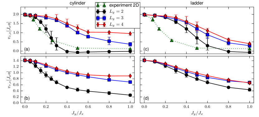
Figure 8: (Color online) (a),(c) Core expansion velocities $v_{c,x}$ and (b),(d) radial velocities $v_{r,x}$ versus $J_{y}$ for the expansion of a $6\times L_{y}$ block. The left panels (a) and (b) are obtained on $L_{y}=2,3,4$ cylinders; the right panels (c),(d) are obtained on $L_{y}=2,3,4$ ladders. The green triangles taken from Ref. Ronzheimer et al. (2013) show the results of the experiments for the fully 2D expansion corresponding to the setup of Sec. V.

Whether propagating modes with $E_{y}=0$ exist or not depends not only on $L_{y}$ but also on the boundary conditions in the $y$ direction. This can serve as a test for our reasoning. For $L_{y}=4$, we find modes with $E_{y}=0$ on a cylinder but not on a ladder (see Appendix B). We compare $\Delta N$ for these two geometries directly in Figs. 7(b) and 7(c). For small $J_{y}/J_{x}=0.2$, the additional coupling of the cylinders compared to the ladders has (at least on the time scales accessible to us) nearly no influence. Yet, for large $J_{y}/J_{x}$, we find not only a quantitative but even a qualitative difference: For the $L_{y}=4$ cylinders, $\Delta N$ increases linearly in time, irrespective of how large $J_{y}/J_{x}$ is. Moreover, the slope is (at $t\gtrsim 1.5\,J_{x}^{-1}$) roughly the same for all $J_{y}/J_{x}\gtrsim 0.5$ and does almost not decrease with time. Using Eq. (9), we can relate this to the presence of a non-decaying current, which we explain in terms of an enhanced occupation at momenta compatible with $E_{y}=0$. In contrast, on the four-leg ladder there are no propagating modes with $E_{y}=0$; thus, we expect no linear increase of $\Delta N$. Indeed, we find that the currents—i.e., the slopes of $\Delta N$ in Fig. 7(c)—on the four-leg ladder decay in time. Yet, the decay is not as extreme as for the two-leg ladder, which we explain by the existence of modes with lower energies $E_{y}>0$ than on the two-leg ladder. For $L_{y}=3$, it is exactly the other way around: There are modes with $E_{y}=0$ on the ladder but not on the cylinder. In agreement with this, Fig. 7(c) shows that the expansion on a three-leg ladder is faster than on an $L_{y}=3$ cylinder for large $J_{y}/J_{x}=2$.

VI.4 Expansion velocities

Figure 8 shows the radial and core velocities for the expansion of blocks on cylinders and ladders. We note that, while $v_{c}$ and $v_{r}$ are nearly independent of $J_{y}/J_{x}$ in the range $J_{y}/J_{x}=0.6,\dots,1$ for the $L_{y}=4$ cylinder [Figs. 8(a) and 8(b)], the values $r_{c}(t)$ and $\tilde{R}(t)$ themselves actually do decrease when $J_{y}/J_{x}$ is tuned from 0.6 to 1 (see Figs. 12 and 13 in the Appendixes), due to different short-time dynamics. Further, for the accessible times ($t_{m}=3\,J_{x}^{-1}$ for $L_{y}=4$), the density profile outside the original block is still completely equivalent to the domain-wall melting. Nevertheless, $r_{c}(t)$, by definition, is also sensitive to the maximum value in the center of the block, and $\tilde{R}(t)$ is sensitive to the densities at all positions. Thus, the velocities shown in Fig. 8 contain valuable and complementary information.

The two-leg ladder (for which the expansion velocity has been studied in Ref. Vidmar et al. (2013)) shows a behavior similar to the experimental data for 2D expansions Ronzheimer et al. (2013), namely that the core velocity $v_{c}$ drops down to zero with increasing $J_{y}/J_{x}$. However, by comparing different $L_{y}$, we find a trend towards a faster expansion when $L_{y}$ is increased at fixed $J_{y}/J_{x}$. This trend is in contrast to the naive expectation that wider cylinders should mimic the 1D-to-2D crossover better. In other words, it demonstrates that the two-leg ladder does not capture all the relevant physics of the expansion in all directions in the 1D-to-2D crossover, although it shows the same qualitative dependence of velocities on $J_{y}/J_{x}$ as the 2D system studied experimentally Ronzheimer et al. (2013). However, we understand this from our considerations of the limit $J_{y}\gg J_{x}$ in Sec. VI.3: On the $L_{y}=4$ cylinder and the $L_{y}=3$ ladder, there exist $E_{y}=0$ modes, and thus a preferred occupation of these propagating modes with nonzero $k_{y}$ is possible. Moreover, in those other cases in which there are no modes with strictly $E_{y}=0$, there are at least modes with lower $|E_{y}|<J_{y}$.

VI.5 Momentum distribution function

The momentum distribution $n_{k_{x},k_{y}}$ on cylinders starting from $6\times L_{y}$ blocks and at fixed time $t=2.0\,J_{x}^{-1}$ is shown in Fig. 9. At small $J_{y}/J_{x}=0.2$, we observe a bunching of particles at the $k_{x}=\pm\frac{\pi}{2a}$ modes independent of $k_{y}$, similar to the fully 2D expansion at the same value of $J_{y}/J_{x}$ shown in Fig. 4.

For $J_{y}=J_{x}$ and on the $L_{y}=3$ cylinder, the energy $E_{y}(k_{y}=\pm\frac{2\pi}{3a})=J_{y}$ can be compensated by kinetic energy $E_{x}=-2J_{x}\cos(k_{x}a)$ in the $x$ direction; compare Eq. (8). Indeed, we find a bunching of particles at those momenta in Fig. 9(e). The $E_{y}(k_{y}=0)=-2J_{y}$ and $E_{y}(k_{y}=\frac{\pi}{a})=2J_{y}$ mode would yield $k_{x}=\frac{\pi}{a}$ and $k_{y}=0$, yet we find a slightly higher weight at smaller $k_{x}$ in Fig. 9(e). However, we note that all these peaks for $J_{y}=J_{x}$ in Figs. 9(d) and 9(e) are not as high as their counterparts for $J_{y}/J_{x}=0.2$. As we have discussed above and in Appendix B, there are no modes with $E_{y}=0$ for $L_{y}=2,3$ on cylinders; hence, the maxima in $n_{k_{x},k_{y}}$ are generally suppressed as we go from small to large $J_{y}/J_{x}$ for $L_{y}=2,3$.

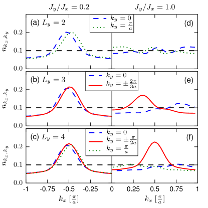
Figure 9: (Color online) Momentum distribution function $n_{k_{x},k_{y}}$ (dimensionless) for cylinders with (a),(d) $L_{y}=2$, (b),(e) $L_{y}=3$ and (c),(f) $L_{y}=4$, starting from a $6\times L_{y}$ cluster. Data are shown for time $t=2.0\,J_{x}^{-1}$ and (a)–(c) $J_{y}/J_{x}=0.2$ and (d)–(f) $J_{y}/J_{x}=1.0$ (Note that we have a symmetry $n_{-k_{x},k_{y}}=n_{k_{x},k_{y}}=n_{k_{x},-k_{y}}$). The black dashed lines indicate the flat initial distribution at $t=0$.

On the $L_{y}=4$ cylinder, we find a bunching of particles at $(k_{x},k_{y})=(\frac{\pi}{2a},\frac{\pi}{2a})$ with roughly the same weight for all $J_{y}$; compare Figs. 9(c) and 9(f). This is in agreement with our considerations of Sec. VI.3, since the modes with $k_{y}=\frac{\pi}{2a}$ have $E_{y}=0$. The $k_{y}=0,\frac{\pi}{a}$ modes are suppressed, similar to the case of $L_{y}=2,3$.

The question of whether the bunching of particles at certain quasimomenta (that requires the existence of propagating modes with energies compatible with those quasimomenta) will lead to a true dynamical quasicondensation at finite momenta can best be addressed using the domain walls as initial stats. Here, we are guided by the behavior of 1D hard-core bosons: In the sudden expansion Rigol and Muramatsu (2004); Vidmar et al. (2013), the dynamical quasicondensation is a transient phenomenon, hence the occupation at $k=\pm\frac{\pi}{2a}$ first increases and then slowly decreases as dynamical fermionization sets in Rigol and Muramatsu (2005b); Minguzzi and Gangardt (2005); Vidmar et al. (2013). The crossover between these two regimes—the formation and the decay of quasicondensates—is given by $t_{2}\propto B$ (see also the discussion in Vidmar et al. (2015)). For the domain-wall melting, the quasicondensates are continuously fed with particles with identical properties due to the presence of an infinite reservoir and thus the quasicondensation peaks in $n_{k}$ never decay but keep increasing.

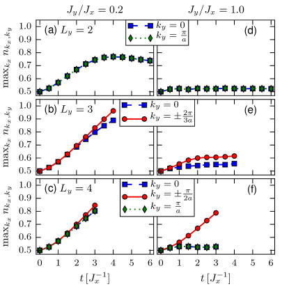
Figure 10: (Color online) Time evolution of the peak heights in the momentum distribution function for cylinders with (a),(d) $L_{y}=2$, (b),(e) $L_{y}=3$, and (c),(f) $L_{y}=4$, starting from a domain wall. Data are shown for (a)–(c) $J_{y}/J_{x}=0.2$ and (d)–(f) $J_{y}/J_{x}=1.0$.

Figure 10 shows the time dependence of the occupation at the maximum of $n_{k_{x},k_{y}}$ for the domain-wall melting on $L_{y}=2,3,4$ cylinders for (a)–(c) $J_{y}/J_{x}=0.2$ and (d)–(f) $J_{y}/J_{x}=1$. For $J_{y}/J_{x}=0.2$ and the accessible time windows of the $L_{y}=3,4$ cylinders, the occupation indeed increases monotonically in time. On the $L_{y}=2$ cylinder in Fig. 10(a), the maximum initially increases similar as for $L_{y}=3,4$, yet for times $t\gtrsim 3J_{x}^{-1}$ it saturates and even decreases, which suggests that no condensation sets in. Note that the time scale at which the saturation happens is quite large, as it is set by $J_{y}^{-1}$. This suggests that there is no condensation even for very small $J_{y}>0$ on the $L_{y}=2$ cylinder.

The behavior for $J_{y}/J_{x}=1$ is quite different. In almost all cases, the occupation at the maximum quickly saturates, which suggests that no condensation sets in. This observation is consistent with the absence of fast propagating modes on the $L_{y}=2,3$ cylinders. Among the data sets shown in Fig. 10(d)–10(f), there is one exception, namely the peak at $(k_{x},k_{y})=(\frac{\pi}{2a},\pm\frac{\pi}{2a})$ on the four-leg cylinder, which monotonically increases without a trend towards saturation. This case is thus the most promising candidate for a condensation at $J_{y}=J_{x}$.

VI.6 Occupation of lowest natural orbital

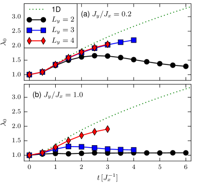
Figure 11: (Color online) Time evolution of the occupation of the largest eigenvalue $\lambda_{0}$ (dimensionless) of the one particle density matrix for cylinders with (a) $J_{y}/J_{x}=0.2$ and (b) $J_{y}/J_{x}=1.0$, starting from a domain wall. The dotted green lines show the results of an 1D chain ($J_{y}=0$) for comparison.

To investigate the question of condensation in more detail, we look at the maximum occupation $\lambda_{0}$ of the natural orbitals Penrose and Onsager (1956). The natural orbitals are effective single particle states defined as the eigenstates of the one particle density matrix $\braket{\hat{a}^{\dagger}_{\mathbf{i}}\hat{a}^{\phantom{\dagger}}_{\mathbf{j}}}$. The corresponding eigenvalues sum up to the number of particles and can be interpreted as the occupations of the natural orbitals. A true condensate requires that $\lambda_{0}$ becomes macroscopically large.

The largest occupation $\lambda_{0}$ for the domain-wall melting of cylinders is shown in Fig. 11. In the 1D case, indicated by the green dotted line, the occupation grows, for large times, as $\lambda_{0}\approx 1.38\sqrt{t}$ Rigol and Muramatsu (2004). For $L_{y}=2$ we find two degenerate natural orbitals with occupation $\lambda_{0}$. For $J_{y}/J_{x}=0.2$, we find an initial growth for all $L_{y}=2,3,4$, but for $L_{y}=2$, the occupation saturates and even decreases for large times $t\gtrsim 3J_{x}^{-1}$, similar as for the peaks in the momentum distribution function. In fact, the peaks in the momentum distribution are directly related to the natural orbitals with the largest occupation: For $L_{y}=2$ there are two degenerate natural orbitals with maximal occupation with $k_{y}=0$ and $k_{y}=\frac{\pi}{a}$, and their Fourier transformation is peaked slightly above (below) $k_{x}=\frac{\pi}{2a}$ for $k_{y}=0$ ($k_{y}=\frac{\pi}{a}$). Similarly, for $L_{y}=3$ ($L_{y}=4$) there are two natural orbitals with maximal occupation with $k_{y}=\pm\frac{2\pi}{3a}$ ($k_{y}=\pm\frac{\pi}{2a}$) and one (two) with slightly lower occupation with $k_{y}=0$ ($k_{y}=0,\frac{\pi}{a}$), leading to the peak structure of Figs. 9(b) and 9(c) (with peaks only at $k_{x}>0$ for domain-wall initial states).

For $J_{y}=J_{x}$, shown in Fig. 11(b), $\lambda_{0}$ saturates and even decreases for the cylinders of width $L_{y}=2,3$, but keeps growing monotonically for $L_{y}=4$ (at least on the time scale accessible to us), in accordance with Figs. 9(f) and 10(f). For $L_{y}=4$, we find only two (degenerate) natural orbitals with $k_{y}=\pm\frac{\pi}{2a}$ with peaks at $k_{x}=\frac{\pi}{2a}$. Yet the maximal occupation $\lambda_{0}$ is significantly smaller than in the 1D case and seems to saturate at larger times.

It is instructive to compare $\lambda_{0}$ to the number of particles in the expanding cloud $\Delta N$ shown in Fig. 7, defining a condensate fraction $\lambda_{0}/\Delta N$. $\Delta N$ increases linearly in time in 1D; hence, the condensate fraction goes to zero with $1/\sqrt{t}$, consistent with the absence of true long-range order. In the case of cylinders, we never observe a saturation of $\lambda_{0}/\Delta N$ to a constant nonzero value, but it keeps decreasing as a function of time. Therefore, a true condensation is not supported by the existing data on any cylinder. Yet the survival of a quasicondensation on the cylinders is consistent with our data.

VII Summary

Motivated by recent experiments with ultracold bosons in an optical lattice Ronzheimer et al. (2013); Vidmar et al. (2015), we simulated the sudden expansion of up to $4\times 4$ hard-core bosons in a 2D lattice. In the limit $J_{x}\gg J_{y}$, we find a fast expansion (at least on the time scale accessible to us), similar to the 1D case. When $J_{y}$ is tuned to the isotropic limit $J_{x}=J_{y}$, some fraction of the particles remains as a high-density core in the center and a spherically symmetric shape emerges. This trend is compatible with the observations made in the experiment of Ref. Ronzheimer et al. (2013). Unfortunately, our results for the 2D expansion are dominated by surface effects due to the small boson numbers as, in fact, in our simulations we have more particles at the boundary of the initial block than in the bulk. This prevents us from analyzing the core expansion velocity Ronzheimer et al. (2013), yet the radial velocities $v_{r,x}$ decrease monotonically with the block size $B$ at any fixed $J_{y}/J_{x}$. We observe a bunching in the momentum distribution function at quasimomenta compatible with energy conservation. This bunching could signal a dynamical condensation at finite quasimomenta as in the 1D case, where this dynamical quasicondensation Rigol and Muramatsu (2004) has recently been observed in an experiment Vidmar et al. (2015). Although we cannot ultimately clarify the question of dynamical condensation in 2D with our small clusters, we believe that the bunching of particles at certain finite momenta in the 2D expansion $J_{y}\approx J_{x}$ stems from surface effects.

In order to investigate the dimensional crossover further, we studied the expansion on long cylinders and ladders with up to $L_{y}=4$ legs. Correlations between the particles in different legs, which lead to a $J_{y}$ dependence, built up on a very short timescale of about one tunneling time in the longitudinal $x$ direction. Up to a time $t_{2}$ that is proportional to the linear dimension of the initial block, the expansion of blocks, restricted to either the left or right half of the system, is identical to the domain-wall melting. On two-leg ladders, the density in the central region becomes very weakly time dependent and almost stationary for $J_{y}/J_{x}\gtrsim 1$, even for the domain walls. This is reflected by a vanishing or even slightly negative core velocity, similar to the observations made in experiments Schneider et al. (2012); Ronzheimer et al. (2013). By considering the limit $J_{y}\gg J_{x}$, we argue that this suppressed expansion on the two-leg ladder for large $J_{y}/J_{x}$ stems from the fact that there are no modes with $E_{y}=0$ on single rungs. For cylinders and ladders with larger $L_{y}\in\set{3,4}$, we generically find a faster expansion with higher velocities than in the $L_{y}=2$ case. Additionally, there is a dependence of expansion velocities on the boundary conditions in the $y$ direction. For instance, the expansion on $L_{y}=4$ cylinder is faster than on a four-leg ladder. In agreement with our considerations of the limit $J_{y}\gg J_{x}$, this is accompanied by a bunching at preferred momenta $k_{y}=\pm\frac{\pi}{2a}$ and $k_{x}=\pm\frac{\pi}{2a}$ and an increasing occupation of natural orbitals. Yet our data does not support a true condensation on any cylinder.

Finally, we state the interesting question whether the expansion velocities on cylinders or ladders will ever show the same dependence on $J_{y}/J_{x}$ as the width $L_{y}$ increases compared to the expansion of a 2D block. The obvious difference is that we fill the cylinders and ladders completely in the $y$ direction. Due to symmetry, the expansion on cylinders is restricted to be along the $x$ direction and, as such, closer to the 1D case, at least for small $L_{y}$. There can thus be two scenarios: Either, even for $L_{y}\rightarrow\infty$, the velocities of the cylinders might well be above the experimental results or, as $L_{y}$ increases beyond $L_{y}=4$, the velocities at a fixed $J_{y}/J_{x}$ will depend nonmonotonically on $L_{y}$.

Further insight into these questions, i.e., the dependence on $L_{y}$ or the question of dynamical condensation at finite momenta in dimensions higher than one, could be gained from future experiments with access to measuring the radius. This could be accomplished using single-site resolution techniques; see Preiss et al. (2015); Fukuhara et al. (2013a, b) for work in this direction.

Acknowledgments. We are indebted to M. Rigol for valuable comments on a previous version of the manuscript. We acknowledge useful discussions with I. Bloch, L. Pollet, M. Rigol, U. Schneider, and L. Vidmar. F.H.-M. was supported by DFG (Deutsche Forschungsgemeinschaft) Research Unit FOR 1807 through Grant No. HE 5242/3-1. This work was also supported in part by National Science Foundation Grant No. PHYS-1066293 and the hospitality of the Aspen Center for Physics.

Appendix A Extraction of core and radial velocity

Both velocities $v_{r}=\frac{\partial\tilde{R}(t)}{\partial t}$ and $v_{c}=\frac{\partial r_{c}(t)}{\partial t}$ are time derivatives of quantities which are not strictly linear in time. Thus, both $v_{r}$ and $v_{c}$ themselves are time dependent. Figure 12 shows the time dependence of the reduced radius $\tilde{R}(t)$, while Fig. 13 shows the core radius $r_{c}(t)$. In the ideal case we would expect them to get constant in the long-time limit. Unfortunately, our calculations are limited to finite times $t_{m}=6\,J_{x}^{-1}$ for the two-leg ladder, $t_{m}\approx 4\,J_{x}^{-1}$ for $L_{y}=3$ cylinders/ladders, $t_{m}\approx 3\,J_{x}^{-1}$ for $L_{y}=4$ cylinders/ladders, and just $t_{m}\approx 1.5\,J_{x}^{-1}$ for the 2D lattice.

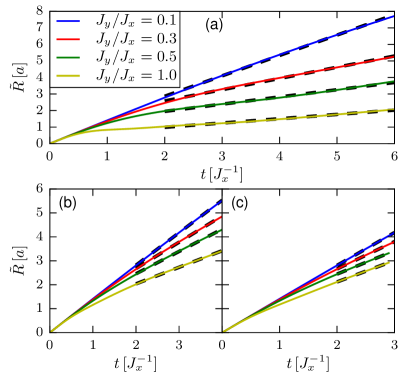
Figure 12: (Color online) Reduced radius $\tilde{R}(t)$ for cylinders with (a) $L_{y}=2$, (b) $L_{y}=3$, and (c) $L_{y}=4$, starting from a $6\times L_{y}$ cluster. The thick dashed lines show the linear fits used to extract the radial velocities $v_{r}$, which are shown in Fig. 8(b).

The reduced radii all start as $\tilde{R}(t)=\sqrt{2}tJ_{x}a$ on very short time scales $t\lesssim 0.5\,J_{x}^{-1}$. This is clear as we are initially confined to the hopping in the $x$ direction, independently of $J_{y}$. For very small $J_{y}\ll J_{x}$, the reduced radius remains linear in time with the velocity $v_{r}=\sqrt{2}J_{x}a$ at all times, as expected for a ballistic expansion from an initial state with a flat quasimomentum distribution function Langer et al. (2012); Ronzheimer et al. (2013). A $J_{y}$ dependence may show up on a timescale $t\propto J_{y}^{-1}$. For larger $J_{y}$ the slope $v_{r}$ reduces at intermediate times (in the time range where we can observe it) but increases again for large $tJ_{x}$. The latter can be understood as follows: The outermost parts have the strongest contribution to the sum in Eq. (3), and naturally these outer parts have the highest velocity $2\,J_{x}a$ (and also reached a low density such that they are dilute and thus do not see each other any more). Assuming a fraction $p$ of the particles to expand with $v$ and the rest $(1-p)$ to form an inert time-independent block in the center (see also the argument given in Sorg et al. (2014)), a straightforward calculation shows that $\tilde{R}(t)\approx\sqrt{p}\,v\,t$ at large times. This is also the reason why $\tilde{R}(t)$ does not settle to a constant value on the two-leg ladder even for large $J_{y}$, although the core in the center barely melts and $\Delta N$ becomes only weakly time dependent: There is always a nonzero fraction of particles which go out from the center.

We extract the time-independent expansion velocities $v_{r}$ shown in Figs. 3 and 8 by a linear fit $\tilde{R}(t)=v_{r}\cdot t+\mathrm{const}$ in the time interval $2.0\,J_{x}^{-1}\leq t\leq t_{m}$, where $t_{m}$ is the maximum time reached in the simulations; see the above. For the 2D lattice, we reach only $t_{m}=1.5\,J_{x}^{-1}$; thus, we fit only in the interval $1.0\,J_{x}^{-1}\leq t\leq 1.5\,J_{x}^{-1}$ in this case. In Fig. 8 we show error bars resulting from similar fits but using only the first or the second half of the time interval.

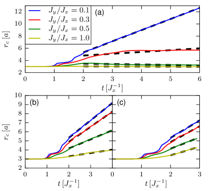
Figure 13: (Color online) Core radius $r_{c}(t)$ for cylinders with (a) $L_{y}=2$, (b) $L_{y}=3$, and (c) $L_{y}=4$, starting from a $6\times L_{y}$ cluster. The thick dashed lines show the linear fits used to extract the core velocities $v_{c}$, which are shown in Fig. 8(a).

In the time regime $0<t<t_{2}$, the core radius is constant, although the cloud already expands: From both edges, the block melts, but the location of the half-maximum density does not move due to particle-hole symmetry. Just when the first holes arrive in the center of the block, the global maximum decreases and $r_{c}$, the half width at half maximum, begins to increase. It then exhibits strong initial oscillations. The latter stem, on the one hand, from the discreteness of the particles’ coordinates on the lattice, which is only partly cured by the linear splines used to extract $r_{c}$. On the other hand, the melting of domain walls in 1D happens in quantized “charges,” which lead to well-defined structures in the density profile Gobert et al. (2005); Hunyadi et al. (2004); Eisler and Rácz (2013). Those oscillations prevent us from extracting the core velocity for the 2D lattice, where they are too strong at the times reached in the simulations. Yet it seems reasonable to extract $v_{c}$ for the cylinders and ladders by linear fits $r_{c}(t)=v_{c}\cdot t+\mathrm{const}$ in the same way as for $v_{r}$. While it works quite well for the ballistic expansion at $J_{y}\ll J_{x}$ and quite large $J_{y}\gtrsim J_{x}$, $r_{c}(t)$ still exhibits a stronger time dependence for intermediate $J_{y}$, e.g., $J_{y}\approx 0.3J_{x}$ on the $L_{y}=2$ cylinder. In the latter case, some of the bosons expand initially during the domain-wall melting and thus the block and $r_{c}$ grow, yet then the expansion is slowed down and the extension of the high-density block measured by $r_{c}$ becomes weakly time dependent.

Appendix B Limit of large $J_{y}\gg J_{x}$

We split the Hamiltonian (1) into two parts according to $H=\sum_{i_{x}}(H^{y}_{i_{x}}+H^{x}_{i_{x},i_{x}+1})$, where $H^{y}_{i_{x}}=-J_{y}\sum_{i_{y}}(\hat{a}^{\dagger}_{i_{x},i_{y}}\hat{a}^{\phantom{\dagger}}_{i_{x},i_{y}+1}+h.c.)$ collects the hopping terms within the rung $i_{x}$ and $H^{x}_{i_{x},i_{x}+1}$ collects the hopping terms between neighboring rungs.

B.1 Two-leg ladder

In the following we give an explicit expression for $H^{x}_{i_{x},i_{x}+1}$ on a two-leg ladder in terms of the eigenstates of $H^{y}_{i_{x}}$ and $H^{y}_{i_{x}+1}$. We denote the four eigenstates of $H^{y}_{i_{x}}$ on rung $i_{x}$ as

$$\ket{0} =\ket{\rm vac}, \ket{1^{+}} =\frac{\hat{a}^{\dagger}_{i_{x},1}+\hat{a}^{\dagger}_{i_{x},2}}{\sqrt{2}}\ket{\rm vac},$$

$$\ket{2} =\hat{a}^{\dagger}_{i_{x},2}\hat{a}^{\dagger}_{i_{x},1}\ket{\rm vac}, \ket{1^{-}} =\frac{\hat{a}^{\dagger}_{i_{x},1}-\hat{a}^{\dagger}_{i_{x},2}}{\sqrt{2}}\ket{\rm vac},$$ (A10)

where $\ket{\rm vac}$ denotes the vacuum on rung $i_{x}$. The corresponding eigenenergies $E_{y}$ of $H^{y}_{i_{x}}$ are listed in Tab. A1. We then express $\hat{a}^{\phantom{\dagger}}_{i_{x},i_{y}}$ and $\hat{a}^{\dagger}_{i_{x},i_{y}}$ in terms of these eigenstates, plug them into $H^{x}_{i_{x},i_{x}+1}$ and obtain:

$$\begin{split}-H^{x}_{i_{x},i_{x}+1}/J_{x}&=\ket{0;1^{+}}\bra{1^{+};0}+\ket{0;1^{-}}\bra{1^{-};0}\\ &+\ket{2;1^{+}}\bra{1^{+};2}+\ket{2;1^{-}}\bra{1^{-};2}\\ &+\ket{1^{+};1^{+}}\bra{0;2}-\ket{1^{-};1^{-}}\bra{0;2}\\ &+\ket{1^{+};1^{+}}\bra{2;0}-\ket{1^{-};1^{-}}\bra{2;0}\\ &+h.c.\,.\end{split}$$ (A11)

Here, $\ket{\alpha;\beta}\equiv\ket{\alpha}\otimes\ket{\beta}$ with $\alpha,\beta\in\set{0,1^{+},1^{-},2}$ denotes the tensorproduct of the eigenstates on rungs $i_{x}$ and $i_{x}+1$. The terms in the first two lines of Eq. (A11) correspond to just an exchange of the eigenstates $\alpha\leftrightarrow\beta$ between the neighboring sites. Thus we can identify the terms of the first line to drive the propagation of single bosons on top of the vacuum. The second line can be seen as the propagation of a particle on top of a one-particle background, or alternatively, a single hole in the background of filled rungs.

In contrast to the terms of the first two lines, the terms in the third and fourth row of Eq. (A11) mix different eigenstates. If we imagine to start from a domain wall $\ket{\dots;2;2;0;0;\dots}$, those are the terms which “create” the single particle modes $\ket{1^{\pm}}$ at the border of the domain wall. Subsequently, we would imagine these modes to propagate away to the left as single-hole modes and to the right as single-boson modes. Yet, for the two-leg ladder all these mixing terms change the total energy $E_{y}$ from $0$ to either $+2J_{y}$ or $-2J_{y}$. Thus, the creation is only possible via higher-order processes, which are suppressed with increasing $J_{y}/J_{x}$. A term such as $\ket{1^{+};1^{-}}\bra{2;0}$ would not change the total energy $E_{y}$, but such a term is not present in Eq. (A11) due to the conservation of total momentum $k_{y}$: it would change from $k_{y}=0+0$ to $k_{y}=0+\frac{\pi}{a}$.

To summarize, we argue that the $L_{y}=2$ ladder is special as it possesses the two extremal modes $k_{y}=0$ and $\pi$ with a large energy $E_{y}=\pm J_{y}$ for one particle on a rung. Note that energy conservation for large $J_{y}\gg J_{x}$ does not suppress the propagation of the modes $\ket{1^{\pm}}$ in the vacuum, but the creation of these modes at the edges of the initial blocks or a domain wall. As a consequence the current decays very rapidly as evidenced in Fig. 7(a).

$L_{y}=2$ ladder
$N$	$k_{y}\,[\frac{\pi}{a}]$	$E_{y}\,[J_{y}]$	state
0	0	0	$\ket{0}$
1	0	-1	$\ket{1^{+}}$
	1	1	$\ket{1^{-}}$
2	0	0	$\ket{2}$

$L_{y}=4$ cylinder
$N$	$k_{y}\,[\frac{\pi}{a}]$	$E_{y}\,[J_{y}]$
0; 4	0	0
1; 3	0	-2
	0.5	0
	-0.5	0
	1	2
2	0	-2.828
	0.5	0
	-0.5	0
	1	0
	1	0
	0	2.828

$L_{y}=4$ ladder
$N$	$E_{y}\,[J_{y}]$
0; 4	0
1; 3	-1.618
	-0.618
	0.618
	1.618
2	-2.236
	-1
	0
	0
	1
	2.236

Table A1: Eigenenergies of a single rung. For a given particle number, degenerate levels are listed by their multiplicity.

B.2 Larger cylinders and ladders

We turn now to the cylinder and the ladder with $L_{y}=4$. The eigenenergies of $H^{y}_{i_{x}}$ on a single rung are listed in Tab. A1. Giving an explicit expression for $H^{x}_{i_{x},i_{x}+1}$ on an $L_{y}=4$ cylinder or ladder is not possible here, since it contains too many terms. Nevertheless, we examine its structure. Similar to that for the two-leg ladder, we can distinguish between terms which just exchange the eigenstates of neighboring rungs and terms which mix them. As on the two-leg ladder, we associate the exchange terms with the propagation of modes. Since $H^{x}$ contains only single-particle hopping, the exchange terms appear only between eigenstates with $N$ and $N+1$ bosons on neighboring rungs. Thus, to first order in $J_{x}/J_{y}$, a mode of $N$ bosons can propagate “freely” only in a background of $N\pm 1$ bosons per rung. By definition, all these exchange terms do not change the total energy $E_{y}$.

For the mixing terms, there is no restriction on the initial particle numbers on the neighboring rungs. However, $H^{x}_{i_{x},i_{x}+1}$ obviously preserves the total number of particle, thus there are only mixing terms for $\ket{\dots N,N^{\prime}\dots}\leftrightarrow\ket{\dots N\pm 1;N^{\prime}\mp 1\dots}$. The initial melting of the edge thus happens via a cascade of subsequent mixing processes. For example, consider

$$\ket{\dots 4;4;0;0\dots}\rightarrow\ket{\dots 4;3;1;0\dots}\rightarrow\ket{\dots 4;2;2;0\dots}\\ \rightarrow\ket{\dots 3;3;2;0\dots}\rightarrow\ket{\dots 3;3;1;1\dots}\,.$$ (A12)

On the cylinder there are states with $E_{y}=0$ for any number of bosons per rung (see Tab. A1). This makes it plausible that cascades like (A12) are possible without changing $E_{y}$ on the single rungs. Indeed, we find the corresponding terms in the expression for $H^{x}_{i_{x},i_{x}+1}$ (not given here). The initial edge of a block or domain wall can thus gradually melt into states with one particle per rung while preserving the energy $E_{y}$. This is confirmed by a strong peak in the momentum distribution function depicted in Fig. 9(f). These additional $k_{y}=\pm\frac{\pi}{2a}$ modes with $E_{y}=0$, which are not present in the two-leg ladder, explain thus the trend of a faster expansion seen as higher velocities in Fig. 8. Moreover, we stress that this process is independent of $J_{y}$, provided that other modes with $E_{y}\neq 0$ are suppressed and our picture is applicable. Indeed, we find that the velocities in Fig. 8 and currents (slopes) in Fig. 7(b) are roughly independent of $J_{y}/J_{x}$, even for moderate $J_{y}/J_{x}\gtrsim 0.6$.

On the other hand, on the four-leg ladder, there are no states with $E_{y}=0$ for one or three bosons on a rung. It is thus immediately clear that there can be no mixing terms which preserve $E_{y}$ on every rung separately. Moreover, we find that there are also no mixing terms which create modes with opposite energy starting from $E_{y}=0$ on both rungs. As a consequence, the domain wall melting on the four-leg ladder requires higher-order processes, similar to the two-leg ladder. However, the necessary intermediate energies $E_{y}=\pm 0.613\times 2J_{y}$ are smaller than for the two-leg ladder, such that these higher-order processes processes are more likely. This is reflected in Fig. 8 by higher velocities for the four-leg ladder compared to the two-leg ladder.

References

- Bloch et al. (2008) I. Bloch, J. Dalibard, and W. Zwerger, Rev. Mod. Phys. 80, 885 (2008).
- Langen et al. (2015a) T. Langen, R. Geiger, and J. Schmiedmayer, Annual Rev. of Condensed Matt. Phys. 6, 201 (2015a).
- Gogolin and Eisert (2015) C. Gogolin and J. Eisert, (2015), arXiv:1503.07538 [quant-ph] .
- Eisert et al. (2015) J. Eisert, M. Friesdorf, and C. Gogolin, Nature Phys. 11, 124 (2015).
- Greiner et al. (2002) M. Greiner, O. Mandel, T. Hänsch, and I. Bloch, Nature (London) 419, 51 (2002).
- Kinoshita et al. (2006) T. Kinoshita, T. Wenger, and S. D. Weiss, Nature (London) 440, 900 (2006).
- Hofferberth et al. (2007) S. Hofferberth, I. Lesanovsky, B. Fisher, T. Schumm, and J. Schmiedmayer, Nature (London) 449, 324 (2007).
- Trotzky et al. (2012) S. Trotzky, Y.-A. Chen, A. Flesch, I. P. McCulloch, U. Schollwöck, J. Eisert, and I. Bloch, Nature Phys. 8, 325 (2012).
- Gring et al. (2012) M. Gring, M. Kuhnert, T. Langen, T. Kitagawa, B. Rauer, M. Schreitl, I. Mazets, D. A. Smith, E. Demler, and J. Schmiedmayer, Science 337, 1318 (2012).
- Cheneau et al. (2012) M. Cheneau, P. Barmettler, D. Poletti, M. Endres, P. Schauß, T. Fukuhara, C. Gross, I. Bloch, C. Kollath, and S. Kuhr, Nature (London) 481, 484 (2012).
- Pertot et al. (2014) D. Pertot, A. Sheikhan, E. Cocchi, L. A. Miller, J. E. Bohn, M. Koschorreck, M. Köhl, and C. Kollath, Phys. Rev. Lett. 113, 170403 (2014).
- Will et al. (2015) S. Will, D. Iyer, and M. Rigol, Nature Communications 6, 6009 (2015).
- Braun et al. (2015) S. Braun, M. Friesdorf, S. S. Hodgman, M. Schreiber, J. P. Ronzheimer, A. Riera, M. del Rey, I. Bloch, J. Eisert, and U. Schneider, Proceedings of the National Academy of Sciences 112, 3641 (2015).
- Langen et al. (2015b) T. Langen, S. Erne, R. Geiger, B. Rauer, T. Schweigler, M. Kuhnert, W. Rohringer, I. E. Mazets, T. Gasenzer, and J. Schmiedmayer, Science 348, 207 (2015b).
- Xia et al. (2014) L. Xia, L. A. Zundel, J. Carrasquilla, A. Reinhard, J. M. Wilson, M. Rigol, and D. S. Weiss, Nature Phys. 11, 316 (2014).
- Vidmar et al. (2015) L. Vidmar, J. P. Ronzheimer, M. Schreiber, S. Braun, S. S. Hodgman, S. Langer, F. Heidrich-Meisner, I. Bloch, and U. Schneider, Phys. Rev. Lett. 115, 175301 (2015).
- Schneider et al. (2012) U. Schneider, L. Hackermüller, J. P. Ronzheimer, S. Will, S. Braun, T. Best, I. Bloch, E. Demler, S. Mandt, D. Rasch, and A. Rosch, Nature Phys. 8, 213 (2012).
- Reinhard et al. (2013) A. Reinhard, J.-F. Riou, L. A. Zundel, D. S. Weiss, S. Li, A. M. Rey, and R. Hipolito, Phys. Rev. Lett. 110, 033001 (2013).
- Ronzheimer et al. (2013) J. P. Ronzheimer, M. Schreiber, S. Braun, S. S. Hodgman, S. Langer, I. P. McCulloch, F. Heidrich-Meisner, I. Bloch, and U. Schneider, Phys. Rev. Lett. 110, 205301 (2013).
- Hild et al. (2014) S. Hild, T. Fukuhara, P. Schauß, J. Zeiher, M. Knap, E. Demler, I. Bloch, and C. Gross, Phys. Rev. Lett. 113, 147205 (2014).
- Giamarchi (2004) T. Giamarchi, Quantum Physics in One Dimension (Clarendon Press, Oxford, 2004) p. 2905.
- Essler et al. (2005) F. Essler, H. Frahm, F. Göhmann, A. Klümper, and V. E. Korepin, The one-dimensional Hubbard model (Cambridge University Press, 2005).
- White (1992) S. R. White, Phys. Rev. Lett. 69, 2863 (1992).
- Schollwöck (2005) U. Schollwöck, Rev. Mod. Phys. 77, 259 (2005).
- Schollwöck (2011) U. Schollwöck, Ann. Phys. (NY) 326, 96 (2011).
- Rigol et al. (2008) M. Rigol, V. Dunjko, and M. Olshanii, Nature (London) 452, 854 (2008).
- Mierzejewski et al. (2011) M. Mierzejewski, L. Vidmar, J. Bonča, and P. Prelovšek, Phys. Rev. Lett. 106, 196401 (2011).
- Bonca et al. (2012) J. Bonca, M. Mierzejewski, and L. Vidmar, Phys. Rev. Lett. 109, 156404 (2012).
- Uhrig (2009) G. S. Uhrig, Phys. Rev. A 80, 061602 (2009).
- Hamerla and Uhrig (2014) S. A. Hamerla and G. S. Uhrig, Phys. Rev. B 89, 104301 (2014).
- Goth and Assaad (2012) F. Goth and F. F. Assaad, Phys. Rev. B 85, 085129 (2012).
- Carleo et al. (2012) G. Carleo, F. Becca, M. Schiró, and M. Fabrizio, Sci. Rep. 2, 243 (2012).
- Carleo et al. (2014) G. Carleo, F. Becca, L. Sanchez-Palencia, S. Sorella, and M. Fabrizio, Phys. Rev. A 89, 031602 (2014).
- Gull et al. (2011) E. Gull, A. J. Millis, A. I. Lichtenstein, A. N. Rubtsov, M. Troyer, and P. Werner, Rev. Mod. Phys. 83, 349 (2011).
- Eckstein et al. (2010) M. Eckstein, A. Hackl, S. Kehrein, M. Kollar, M. Moeckel, P. Werner, and F. A. Wolf, Eur. Phys. J. Special Topics 180, 217 (2010).
- Moeckel and Kehrein (2008) M. Moeckel and S. Kehrein, Phys. Rev. Lett. 100, 175702 (2008).
- Queisser et al. (2014) F. Queisser, K. V. Krutitsky, P. Navez, and R. Schützhold, Phys. Rev. A 89, 033616 (2014).
- Lux et al. (2014) J. Lux, J. Müller, A. Mitra, and A. Rosch, Phys. Rev. A 89, 053608 (2014).
- Lux and Rosch (2015) J. Lux and A. Rosch, Phys. Rev. A 91, 023617 (2015).
- Schützhold et al. (2006) R. Schützhold, M. Uhlmann, Y. Xu, and U. R. Fischer, Phys. Rev. Lett. 97, 200601 (2006).
- Schiró and Fabrizio (2010) M. Schiró and M. Fabrizio, Phys. Rev. Lett. 105, 076401 (2010).
- Schiró and Fabrizio (2011) M. Schiró and M. Fabrizio, Phys. Rev. B 83, 165105 (2011).
- Jreissaty et al. (2011) M. Jreissaty, J. Carrasquilla, F. A. Wolf, and M. Rigol, Phys. Rev. A 84, 043610 (2011).
- Jreissaty et al. (2013) A. Jreissaty, J. Carrasquilla, and M. Rigol, Phys. Rev. A 88, 031606(R) (2013).
- Schlünzen et al. (2015) N. Schlünzen, S. Hermanns, M. Bonitz, and C. Verdozzi, (2015), arXiv:1508.02947 [cond-mat.quant-gas] .
- Yan et al. (2011) S. Yan, D. A. Huse, and S. R. White, Science 332, 1173 (2011).
- Depenbrock et al. (2012) S. Depenbrock, I. P. McCulloch, and U. Schollwöck, Phys. Rev. Lett. 109, 067201 (2012).
- Stoudenmire and White (2012) E. Stoudenmire and S. R. White, Annual Review of Condensed Matter Physics 3, 111 (2012).
- Maeshima et al. (2001) N. Maeshima, Y. Hieida, Y. Akutsu, T. Nishino, and K. Okunishi, Phys. Rev. E 64, 016705 (2001).
- Verstraete and Cirac (2004) F. Verstraete and J. Cirac, (2004), arXiv:cond-mat/0407066 .
- Jordan et al. (2008) J. Jordan, R. Orús, G. Vidal, F. Verstraete, and J. I. Cirac, Phys. Rev. Lett. 101, 250602 (2008).
- Corboz et al. (2011) P. Corboz, S. R. White, G. Vidal, and M. Troyer, Phys. Rev. B 84, 041108 (2011).
- Zaletel et al. (2015) M. P. Zaletel, R. S. K. Mong, C. Karrasch, J. E. Moore, and F. Pollmann, Phys. Rev. B 91, 165112 (2015).
- Dorando et al. (2009) J. J. Dorando, J. Hachmann, and G. K.-L. Chan, The Journal of Chemical Physics 130, 184111 (2009).
- Haegeman et al. (2011) J. Haegeman, J. I. Cirac, T. J. Osborne, I. Pižorn, H. Verschelde, and F. Verstraete, Phys. Rev. Lett. 107, 070601 (2011).
- Lubasch et al. (2011) M. Lubasch, V. Murg, U. Schneider, J. I. Cirac, and M.-C. Bañuls, Phys. Rev. Lett. 107, 165301 (2011).
- James and Konik (2015) A. J. A. James and R. M. Konik, Phys. Rev. B 92, 161111 (2015).
- Vidal (2004) G. Vidal, Phys. Rev. Lett. 93, 040502 (2004).
- (59) A. Daley, C. Kollath, U. Schollwöck, and G. Vidal, J. Stat. Mech.: Theory Exp. (2004), P04005.
- White and Feiguin (2004) S. R. White and A. E. Feiguin, Phys. Rev. Lett. 93, 076401 (2004).
- Brown et al. (2015) R. C. Brown, R. Wyllie, S. B. Koller, E. A. Goldschmidt, M. Foss-Feig, and J. V. Porto, Science 348, 540 (2015).
- Antal et al. (1998) T. Antal, Z. Rácz, A. Rákos, and G. M. Schütz, Phys. Rev. E 57, 5184 (1998).
- Gobert et al. (2005) D. Gobert, C. Kollath, U. Schollwöck, and G. Schütz, Phys. Rev. E 71, 036102 (2005).
- Lancaster and Mitra (2010) J. Lancaster and A. Mitra, Phys. Rev. E 81, 061134 (2010).
- (65) J. Caux and J. Mossel, J. Stat. Mech. (2011), P02023.
- Santos and Mitra (2011) L. F. Santos and A. Mitra, Phys. Rev. E 84, 016206 (2011).
- Sabetta and Misguich (2013) T. Sabetta and G. Misguich, Phys. Rev. B 88, 245114 (2013).
- Halimeh et al. (2014) J. C. Halimeh, A. Wöllert, I. P. McCulloch, U. Schollwöck, and T. Barthel, Phys. Rev. A 89, 063603 (2014).
- Alba and Heidrich-Meisner (2014) V. Alba and F. Heidrich-Meisner, Phys. Rev. B 90, 075144 (2014).
- Vidmar et al. (2013) L. Vidmar, S. Langer, I. P. McCulloch, U. Schneider, U. Schollwöck, and F. Heidrich-Meisner, Phys. Rev. B 88, 235117 (2013).
- Steinigeweg et al. (2014) R. Steinigeweg, F. Heidrich-Meisner, J. Gemmer, K. Michielsen, and H. De Raedt, Phys. Rev. B 90, 094417 (2014).
- Karrasch et al. (2015) C. Karrasch, D. M. Kennes, and F. Heidrich-Meisner, Phys. Rev. B 91, 115130 (2015).
- Muth et al. (2012) D. Muth, D. Petrosyan, and M. Fleischhauer, Phys. Rev. A 85, 013615 (2012).
- Boschi et al. (2014) C. D. E. Boschi, E. Ercolessi, L. Ferrari, P. Naldesi, F. Ortolani, and L. Taddia, Phys. Rev. A 90, 043606 (2014).
- Sorg et al. (2014) S. Sorg, L. Vidmar, L. Pollet, and F. Heidrich-Meisner, Phys. Rev. A 90, 033606 (2014).
- Heidrich-Meisner et al. (2009) F. Heidrich-Meisner, S. R. Manmana, M. Rigol, A. Muramatsu, A. E. Feiguin, and E. Dagotto, Phys. Rev. A 80, 041603 (2009).
- Kajala et al. (2011) J. Kajala, F. Massel, and P. Törmä, Phys. Rev. Lett. 106, 206401 (2011).
- Schönmeier-Kromer and Pollet (2014) J. Schönmeier-Kromer and L. Pollet, Phys. Rev. A 89, 023605 (2014).
- Hen and Rigol (2010) I. Hen and M. Rigol, Phys. Rev. Lett. 105, 180401 (2010).
- Rigol and Muramatsu (2004) M. Rigol and A. Muramatsu, Phys. Rev. Lett. 93, 230404 (2004).
- Rigol and Muramatsu (2005a) M. Rigol and A. Muramatsu, Mod. Phys. Lett. B 19, 861 (2005a).
- Micheli et al. (2004) A. Micheli, A. J. Daley, D. Jaksch, and P. Zoller, Phys. Rev. Lett. 93, 140408 (2004).
- Daley et al. (2005) A. J. Daley, S. R. Clark, D. Jaksch, and P. Zoller, Phys. Rev. A 72, 043618 (2005).
- Rodriguez et al. (2006) K. Rodriguez, S. Manmana, M. Rigol, R. Noack, and A. Muramatsu, New J. Phys. 8, 169 (2006).
- Rigol and Muramatsu (2005b) M. Rigol and A. Muramatsu, Phys. Rev. Lett. 94, 240403 (2005b).
- Minguzzi and Gangardt (2005) A. Minguzzi and D. M. Gangardt, Phys. Rev. Lett. 94, 240404 (2005).
- Fölling et al. (2007) S. Fölling, S. Trotzky, P. Cheinet, M. Feld, R. Saers, A. Widera, T. Müller, and I. Bloch., Nature (London) 448, 1029 (2007).
- Celi et al. (2014) A. Celi, P. Massignan, J. Ruseckas, N. Goldman, I. B. Spielman, G. Juzeliūnas, and M. Lewenstein, Phys. Rev. Lett. 112, 043001 (2014).
- Stuhl et al. (2015) B. K. Stuhl, H.-I. Lu, L. M. Aycock, D. Genkina, and I. B. Spielman, Science 349, 1514 (2015).
- Mancini et al. (2015) M. Mancini, G. Pagano, G. Cappellini, L. Livi, M. Rider, J. Catani, C. Sias, P. Zoller, M. Inguscio, M. Dalmonte, and L. Fallani, Science 349, 1510 (2015).
- Cazalilla et al. (2011) M. A. Cazalilla, R. Citro, T. Giamarchi, E. Orignac, and M. Rigol, Rev. Mod. Phys. 83, 1405 (2011).
- Langer et al. (2012) S. Langer, M. J. A. Schuetz, I. P. McCulloch, U. Schollwöck, and F. Heidrich-Meisner, Phys. Rev. A 85, 043618 (2012).
- Jukić et al. (2009) D. Jukić, B. Klajn, and H. Buljan, Phys. Rev. A 79, 033612 (2009).
- Mei et al. (2015) Z. Mei, L. Vidmar, F. Heidrich-Meisner, and C. J. Bolech, (2015), arXiv:1509.00828 [cond-mat.quant-gas] .
- Verstraete et al. (2004) F. Verstraete, D. Porras, and J. I. Cirac, Phys. Rev. Lett. 93, 227205 (2004).
- Trombettoni and Smerzi (2001) A. Trombettoni and A. Smerzi, Phys. Rev. Lett. 86, 2353 (2001).
- Hennig et al. (2013) H. Hennig, T. Neff, and R. Fleischmann, (2013), arXiv:1309.7939 [nlin.PS] .
- Penrose and Onsager (1956) O. Penrose and L. Onsager, Phys. Rev. 104, 576 (1956).
- Preiss et al. (2015) P. M. Preiss, R. Ma, M. E. Tai, A. Lukin, M. Rispoli, P. Zupancic, Y. Lahini, R. Islam, and M. Greiner, Science 347, 1229 (2015).
- Fukuhara et al. (2013a) T. Fukuhara, A. Kantian, M. Endres, M. Cheneau, P. Schauß, S. Hild, C. Gross, U. Schollwöck, T. Giamarchi, I. Bloch, and S. Kuhr, Nature Phys. 9, 235 (2013a).
- Fukuhara et al. (2013b) T. Fukuhara, P. Schauß, M. Endres, S. Hild, M. Cheneau, I. Bloch, and C. Gross, Nature 506, 76 (2013b).
- Hunyadi et al. (2004) V. Hunyadi, Z. Rácz, and L. Sasvári, Phys. Rev. E 69, 066103 (2004).
- Eisler and Rácz (2013) V. Eisler and Z. Rácz, Phys. Rev. Lett. 110, 060602 (2013).