The (magnetized) effective QCD phase diagram^∗

Abstract

I present the highlights of a recent study of the effective QCD phase diagram on the temperature $T$ and quark chemical potential $\mu$ plane, where the strong interactions are modeled using the linear sigma model coupled to quarks. The phase transition line is found from the effective potential at finite $T$ and $\mu$ taking into account the plasma screening effects. We find the location of the critical end point (CEP) to be $(\mu^{\mbox{\tiny{CEP}}}/T_{c},T^{\mbox{\tiny{CEP}}}/T_{c})\sim(1.2,0.8)$, where $T_{c}$ is the (pseudo)critical temperature for the crossover phase transition at vanishing $\mu$. This location lies within the region found by lattice inspired calculations. Since the linear sigma model does not exhibit confinement, I argue that the location is due to the proper treatment of the plasma screening effects and not to the size of the confining scale. I also comment on the extension of this study to determine the dependence of the CEP’s location on the strength of an external magnetic field.

Nuclear and Particle Physics Proceedings nppp Nuclear and Particle Physics Proceedings

1 Introduction

The different phases in which matter made up of quarks and gluons arranges itself depends on the temperature and density, or equivalently, on the temperature and chemical potentials. The representation of the QCD phase diagram is thus two dimensional. This is customary plotted with the light-quark chemical potential $\mu$ as the horizontal variable and the temperature $T$ as the vertical one. $\mu$ is related to the baryon chemical potential $\mu_{B}$ by $\mu_{B}=3\mu$.

Most of our knowledge of the phase diagram is restricted to the $\mu=0$ axis. The phase diagram is, by and large, unknown. For physical quark masses and $\mu=0$, lattice calculations have shown [1] that the change from the low temperature phase, where the degrees of freedom are hadrons, to the high temperature phase described by quarks and gluons, is an analytic crossover. The phase transition has a dual nature: on the one hand the color-singlet hadrons break up leading to deconfined quarks and gluons; this is dubbed as the deconfinement phase transition. On the other hand, the dynamically generated component of quark masses within hadrons vanishes; this is referred to as chiral symmetry restoration.

Lattice calculations have provided values for the crossover (pseudo)critical temperature $T_{c}$ for $\mu=0$ and 2+1 quark flavors using different types of improved rooted staggered fermions. The MILC collaboration obtained $T_{c}=169(12)(4)$ MeV. The RBC-Bielefeld collaboration reported $T_{c}=192(7)(4)$ MeV. The Wuppertal-Budapest collaboration has consistently obtained smaller values, the latest being $T_{c}=147(2)(3)$ MeV. The HotQCD collaboration has computed $T_{c}=154(9)$ MeV and more recently $T_{c}=155(1)(8)$ MeV [2]. The differences could perhaps be attributed to different lattice spacings.

Although the above picture presented by lattice QCD cannot be easily extended to the case $\mu\neq 0$ due to the sign problem, some mathematical extensions of lattice techniques [3] as well as Schwinger-Dyson equations [4], can be employed to explore all the phase diagram.

A number of different model approaches indicate that the transition along the $\mu$ axis, at $T=0$, is strongly first order [5]. Since the first order line originating at $T=0$ cannot end at the $\mu=0$ axis which corresponds to the starting point of the cross-over line, it must terminate somewhere in the middle of the phase diagram. This point is generally referred to as the critical end point (CEP). The mathematical extensions of lattice techniques place the CEP in the region $(\mu^{\mbox{\tiny{CEP}}}/T_{c},T^{\mbox{\tiny{CEP}}}/T_{c})\sim(1.0-1.4,0.9-0.95)$ [6].

In the first of Refs. [4], it is argued that the theoretical location of the CEP depends on the size of the confining length scale used to describe strongly interacting matter at finite density/temperature. This argument is supported by the observation that the models which do not account for this scale [7, 8, 9, 10] produce either a CEP closer to the $\mu$ axis ($\mu^{\mbox{\tiny{CEP}}}/T_{c}$ and $T^{\mbox{\tiny{CEP}}}/T_{c}$ larger and smaller, respectively) or a lower $T_{c}$ [11] than the lattice based approaches or the ones which consider a finite confining length scale. Given the dual nature of the QCD phase transition, it is interesting to explore whether there are other features in models which have access only to the chiral symmetry restoration facet of QCD that, when properly accounted for, produce the CEP’s location more in line with lattice inspired results.

An important clue is provided by the behavior of the critical temperature as a function of an applied magnetic field. Lattice calculations have found that this temperature decreases when the field strength increases [12, 13, 14]. It has been recently shown that this phenomenon, dubbed inverse magnetic catalysis, can be obtained in models, such as the Abelian Higgs model or the linear sigma model with quarks, which show only chiral symmetry restoration and lack confinement. This result is a consequence of the decrease of the coupling constants with increasing field strength. The novel feature implemented in these calculations is the handling of the screening properties of the plasma, which effectively makes the treatment go beyond the mean field approximation [15, 16] and allows to consider the thermomagnetic modifications of the coupling constants at lowest order within the same calculation. Screening is also important to obtain a decrease of the coupling constant with the magnetic field strength in QCD in the Hard Thermal Loop approximation [17].

It therefore seems that properly accounting for the plasma screening effects in effective models allows to obtain both a CEP’s location in line with lattice inspired techniques as well as inverse magnetic catalysis. A pertinent question is what happens to the CEP’s location once a magnetic field dependence is included in the analysis for $\mu\neq 0$ and wether the nature of the phase transition for $\mu=0$ changes as the magnetic field strength increases. Recent lattice QCD calculations [18] show that at very high values of the magnetic field strength, inverse magnetic catalysis prevails and that the phase transition becomes first order at asymptotically large values of the magnetic field for $\mu=0$ (see also Ref. [19]). In this work we explore the consequences of the proper handling of the plasma screening properties in the description of the effective QCD phase diagram within the linear sigma model with quarks. We argue that it is the adequate description of these properties which determines the CEP’s location. We find that for certain values of the model parameters, obtained from physical constraints, the CEP’s location agrees with lattice inspired calculations. We also give a preview of work in progress [20] that shows that when including the effects of a magnetic field in the calculation of both the effective potential as well as on the thermomagnetic dependence of the coupling constants, the CEP’s location moves toward smaller values of the chemical potential and lower temperatures and that above a certain value of the field strength the CEP reaches the $T$-axis and the phase transitions become first order, also in line with recent lattice results [18]. Details of the calculation that forms the basis of this work can be found in Ref. [21].

2 The linear sigma model with quarks

We start from the linear sigma model coupled to quarks. It is given by the Lagrangian density

$${\mathcal{L}} = \frac{1}{2}(\partial_{\mu}\sigma)^{2}+\frac{1}{2}(\partial_{\mu}\vec{\pi})^{2}+\frac{a^{2}}{2}(\sigma^{2}+\vec{\pi}^{2})$$ (1)

$$- \frac{\lambda}{4}(\sigma^{2}+\vec{\pi}^{2})^{2}+i\bar{\psi}\gamma^{\mu}\partial_{\mu}\psi$$

$$- g\bar{\psi}(\sigma+i\gamma_{5}\vec{\tau}\cdot\vec{\pi})\psi,$$

where $\psi$ is an SU(2) isospin doublet, $\vec{\pi}=(\pi_{1},\pi_{2},\pi_{3})$ is an isospin triplet and $\sigma$ is an isospin singlet. The neutral pion is taken as the third component of the pion isovector, $\pi^{0}=\pi_{3}$ and the charged pions as $\pi_{\pm}=(\pi_{1}\mp i\pi_{2})/2$. The squared mass parameter $a^{2}$ and the self-coupling $\lambda$ and $g$ are taken to be positive.

To allow for the spontaneous breaking of symmetry, we let the $\sigma$ field develop a vacuum expectation value $v$

$$\sigma\rightarrow\sigma+v,$$ (2)

which can later be taken as the order parameter of the theory. After this shift, the Lagrangian density can be rewritten as

$${\mathcal{L}} = -\frac{1}{2}\sigma\partial_{\mu}\partial^{\mu}\sigma-\frac{1}{2}\left(3\lambda v^{2}-a^{2}\right)\sigma^{2}$$ (3)

$$- \frac{1}{2}\vec{\pi}\partial_{\mu}\partial^{\mu}\vec{\pi}-\frac{1}{2}\left(\lambda v^{2}-a^{2}\right)\vec{\pi}^{2}+\frac{a^{2}}{2}v^{2}$$

$$- \frac{\lambda}{4}v^{4}+i\bar{\psi}\gamma^{\mu}\partial_{\mu}\psi-gv\bar{\psi}\psi+{\mathcal{L}}_{I}^{b}+{\mathcal{L}}_{I}^{f},$$

where ${\mathcal{L}}_{I}^{b}$ and ${\mathcal{L}}_{I}^{f}$ are given by

$${\mathcal{L}}_{I}^{b} = -\frac{\lambda}{4}\Big{[}(\sigma^{2}+(\pi^{0})^{2})^{2}$$

$$+ 4\pi^{+}\pi^{-}(\sigma^{2}+(\pi^{0})^{2}+\pi^{+}\pi^{-})\Big{]},$$

$${\mathcal{L}}_{I}^{f} = -g\bar{\psi}(\sigma+i\gamma_{5}\vec{\tau}\cdot\vec{\pi})\psi,$$ (4)

and describe the interactions among the fields $\sigma$, $\vec{\pi}$ and $\psi$, after symmetry breaking. From Eq. (3) we see that the $\sigma$, the three pions and the quarks have masses

$$m^{2}_{\sigma} = 3\lambda v^{2}-a^{2},$$

$$m^{2}_{\pi} = \lambda v^{2}-a^{2},$$

$$m_{f} = gv,$$ (5)

respectively.

The one-loop effective potential for the linear sigma model with quarks including the plasma screening properties encoded in the ring diagrams contribution has been calculated in detail for zero chemical potential in Refs. [22, 23]. Such analyses show that inclusion of the ring diagrams renders the effective potential stable.

When the $\mu$ is non-vanishing, the calculation of the effective potential is more complicated. Though the boson contribution remains the same, the fermion contribution has to be modified due to the chemical potential. The modification enters the calculation in two ways: indirectly into the boson self-energy and directly from its contribution to the effective potential.

To one-loop order the fermion contribution to the effective potential in the imaginary time formalism of thermal field theory is given by [22]

$$V_{f} \!\!\!\!=\!\!\!\! -\frac{2}{\beta}\int\frac{\mathrm{d}^{3}k}{(2\pi)^{3}}\,\left[\beta\omega+\ln\left(1+\mathrm{e}^{-\beta(\omega-\mu)}\right)\right.$$ (6)

$$\!\!\!\!+\!\!\!\! \left.\ln\left(1+\mathrm{e}^{-\beta(\omega+\mu)}\right)\right],$$

where $\beta=T^{-1}$ and $\omega=(\vec{k}^{2}+m_{f}^{2})^{1/2}$, and the sum over the fermion Matsubara frequencies has been performed. The first term in Eq. (6) corresponds to the vacuum contribution whereas the second and third ones are the matter contributions. Note that the matter contribution is made out of separate quark and antiquark pieces due to the finite chemical potential. The vacuum contribution is well-known [22] and can be expressed, after mass renormalization as a function of the renormalization scale $\tilde{\mu}$. For the evaluation of the medium’s contribution in Eq. (6) we adapt the technique from Ref. [24] to the present case. The main idea is to produce a second-order differential equation in $y^{2}$, where $y=m_{f}/T$, valid at high temperature with $m_{f}$ as the smallest of all scales, for the finite temperature part of the potential, which we denote by $\tilde{V}_{f}$, given in Eq. (6) with appropriate boundary conditions at $y=0$, where the integrals can be analytically evaluated. The expression for the effective potential is obtained by integrating this differential equation and using the given boundary conditions. Combining the vacuum contribution after mass renormalization with the finite temperature part we finally have [21]

$$\tilde{V}_{f} \!\!\!\!=\!\!\!\! -\frac{1}{16\pi^{2}}\left\{m_{f}^{4}\left[\ln\left(\frac{(4\pi T)^{2}}{2\tilde{\mu}^{2}}\right)\right.\right.$$ (7)

$$\!\!\!\!+\!\!\!\! \left.\psi^{0}\left(\frac{1}{2}+\frac{\mathrm{i}\mu}{2\pi T}\right)+\psi^{0}\left(\frac{1}{2}-\frac{\mathrm{i}\mu}{2\pi T}\right)\right]$$

$$\!\!\!\!+\!\!\!\! 8m^{2}T^{2}\left[Li_{2}(-e^{\mu/T})+Li_{2}(-e^{-\mu/T})\right]$$

$$\!\!\!\!-\!\!\!\! \left.32T^{4}\left[Li_{4}(-e^{\mu/T})+Li_{4}(-e^{-\mu/T})\right]\right\}.$$

It can also be shown that the boson self-energy $\Pi$ computed for a finite chemical potential and in the limit where the masses are small compared to $T$, is given by

$$\Pi = \frac{\lambda T^{2}}{2}$$ (8)

$$- \frac{N_{f}N_{c}g^{2}T^{2}}{\pi^{2}}\left[Li_{2}(-e^{\mu/T})+Li_{2}(-e^{-\mu/T})\right],$$

where $N_{f}=2$ and $N_{c}=3$ are the number of light flavors and colors, respectively.

Choosing the renormalization scale as $\tilde{\mu}=e^{-1/2}a$, the effective potential up to the ring diagrams contribution is then given by

$$\!\!\!\!\!\!\!\!V^{({\mbox{\small{eff}}})} \!\!\!\!=\!\!\!\! -\frac{a^{2}}{2}v^{2}+\frac{\lambda}{4}v^{4}$$ (9)

$$\!\!\!\!+\!\!\!\! \sum_{i=\sigma,\vec{\pi}}\left\{\frac{m_{i}^{4}}{64\pi^{2}}\left[\ln\left(\frac{(4\pi T)^{2}}{2a^{2}}\right)\right.\right.$$

$$\!\!\!\!-\!\!\!\! \left.2\gamma_{E}+1\frac{}{}\right]-\frac{\pi^{2}T^{4}}{90}+\frac{m_{i}^{2}T^{2}}{24}$$

$$\!\!\!\!-\!\!\!\! \left.\frac{T}{12\pi}(m_{i}^{2}+\Pi)^{3/2}\right\}$$

$$\!\!\!\!-\!\!\!\! \frac{N_{c}}{16\pi^{2}}\sum_{f=u,d}\left\{m_{f}^{4}\left[\ln\left(\frac{(4\pi T)^{2}}{2a^{2}}\right)+1\right.\right.$$

$$\!\!\!\!+\!\!\!\! \left.\psi^{0}\left(\frac{1}{2}+\frac{i\mu}{2\pi T}\right)+\psi^{0}\left(\frac{1}{2}-\frac{i\mu}{2\pi T}\right)\right]$$

$$\!\!\!\!+\!\!\!\! 8\ m_{f}^{2}T^{2}\left[Li_{2}(-e^{\mu/T})+Li_{2}(-e^{-\mu/T})\right]$$

$$\!\!\!\!-\!\!\!\! \left.32\ T^{4}\left[Li_{4}(-e^{\mu/T})+Li_{4}(-e^{-\mu/T})\right]\right\}.$$

In the limit when $\mu\rightarrow 0$, Eq. (9) becomes the expression found in Refs. [22, 23]. In the same limit, Eq. (8) reduces to the well known expression for the self-energy at high temperature [16]. Equation (9) represents the effective potential computed beyond the mean field approximation that accounts for the leading screening effects at high temperature.

3 The phase diagram

In order to find the values of the parameters $\lambda$, $g$ and $a$ appropriate for the description of the phase transition, we note that when considering the thermal effects the boson masses are modified since they acquire a thermal component. For $\mu=0$ they become

$$m_{\sigma}^{2}(T) = 3\lambda v^{2}-a^{2}+\frac{\lambda T^{2}}{2}+\frac{N_{f}N_{c}g^{2}T^{2}}{6}$$

$$m_{\pi}^{2}(T) = \lambda v^{2}-a^{2}+\frac{\lambda T^{2}}{2}+\frac{N_{f}N_{c}g^{2}T^{2}}{6}.$$ (10)

At the phase transition, the curvature of the effective potential vanishes for $v=0$. Since the boson thermal masses are proportional to this curvature, these also vanish at $v=0$. From any of the Eqs. (10), we obtain a relation between the model parameters at $T_{c}$ given by

$$a=T_{c}\sqrt{\frac{\lambda}{2}+\frac{N_{f}N_{c}g^{2}}{6}}.$$ (11)

Furthermore, we can fix the value of $a$ by noting from Eqs. (5) that the vacuum boson masses satisfy

$$a=\sqrt{\frac{m_{\sigma}^{2}-3m_{\pi}^{2}}{2}}.$$ (12)

Since in our scheme we consider two-flavor massless quarks in the chiral limit, we take $T_{c}\simeq 170$ MeV [25] which is slightly larger than $T_{c}$ obtained in $N_{f}=2+1$ lattice simulations. Also, in order to allow for a crossover phase transition for $\mu=0$ (which in our description corresponds to a second order transition) with $g$, $\lambda\sim 1$ we need that $g^{2}>\lambda$. Since the effective potential is written as an expansion in powers of $a/T$ we need that this ratio is smaller than 1. From Eqs. (11) and (12) the coupling constants are proportional to $m_{\sigma}$ which, from the above conditions, restricts the analysis to considering not too large values of $m_{\sigma}$. Since the purpose of this work is not to pursue a precise determination of the couplings but instead to call attention to the fact that the proper treatment of screening effects allows the linear sigma model to provide solutions for the CEP, we consider small values for $m_{\sigma}$. Given that $\sigma$ is anyhow a broad resonance, in order to satisfy the above requirements let us take for definitiveness $m_{\sigma}=300$ namely, close to the two-pion threshold. Therefore, the allowed values for the couplings $\lambda$ and $g$ are restricted by

$$\sqrt{\frac{\lambda}{2}+\frac{N_{f}N_{c}g^{2}}{6}}=0.77.$$ (13)

Equation (13) provides a relation between $\lambda$ and $g$. A possible solution consistent with the above requirements is given as an illustration by $\lambda=0.2$, $g=0.71$. The corresponding phase diagram thus obtained is shown in Fig. 1.

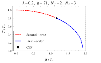
Figure 1: Effective QCD phase diagram computed for $\lambda=0.2$ and $g=0.71$ obtained by considering $m_{\sigma}^{\mbox{\tiny{vac}}}=300$ MeV. For small values of $\mu$ the phase transition is second order. The order of the transition changes to first order for larger values of $\mu$. The CEP is located at $(\mu^{\mbox{\tiny{CEP}}}/T_{c},T^{\mbox{\tiny{CEP}}}/T_{c})\sim(1.2,0.8)$.

Note that for small $\mu$ the phase transition is second order. In this case the (pseudo)critical temperature is determined from setting the second derivative of the effective potential in Eq. (9) to zero at $v=0$. When $\mu$ increases, the phase transition becomes first order. The critical temperature is now computed by looking for the temperature where a secondary minimum for $v\neq 0$ is degenerate with a minimum at $v=0$. In both of these cases, from the detailed analysis, we locate the position of the CEP as $(\mu^{\mbox{\tiny{CEP}}}/T_{c},T^{\mbox{\tiny{CEP}}}/T_{c})\sim(1.2,0.8)$, which is in the same range as the CEP found from lattice inspired analyses [3]. Note also that the phase transition curve is essentially flat close to the $T$ axis.

4 Conclusions

In conclusion, we have shown that it is possible to obtain values for the couplings that allow to locate the CEP in the region found by mathematical extensions of lattice analyses. Since the linear sigma model does not have confinement we attribute this location to the adequate description of the plasma screening properties for the chiral symmetry breaking at finite temperature and density. Magnetic field effects can be included in the description [20] both into the effective potential and into the behavior of the couplings, at lowest order. These last corrections lead to a decreasing of the couplings with the field strength. This decrease can be understood in general terms since the magnetic field produces a dimensional reduction whereby the virtual particles that make up the vacuum are effectively constrained to occupy Landau levels and thus restrict its motion to planes. This produces that charged virtual particles lie closer to each other and thus, because of asymptotic freedom, reduce the strength of the interaction. This happens no matter how weak the external field may be. We have found also that as the field strength increases, the CEP’s location moves to lower values of $\mu$ and of $T$ and that in fact there is a value for this field where the CEP reaches the $T$-axis where the first order phase transitions remain for larger values of the field. These findings will be reported elsewhere shortly. We believe this description will play an important role in determining the location of the CEP also in QCD with and without magnetic fields.

References

- [1] Y. Aoki, G. Endrödi, Z. Fodor, S. K. Katz and K. K. Szabó, Nature 443, 675 (2006).
- [2] L. Levkova, PoS Lattice 2011, 011 (2011); C. Bernard et al. (MILC Collaboration), Phys. Rev. D 71, 034504 (2005); M. Cheng et al., Phys. Rev. D 74, 054507 (2006); S. Borsányi et al., J. High Energy Phys. 1009.073 (2010); Y. Aoki et al., J. High Energy Phys. 0906.088 (2009); Y. Aoki et al., Phys. Lett. B, 643, 46 (2006); A. Bazavov, PoS Lattice 2011, 182 (2011); A. Bazavov et al., Phys. Rev. D 85, 054503 (2012); T. Bhattacharya et al., Phys. Rev. Lett. 113, 082001 (2014).
- [3] Z. Fodor and S. D. Katz, J. High Energy Phys. 0203, 014 (2002); A. Li, A. Alexandru, X. Meng, and K. F. Liu, Nucl. Phys. A830, 633C (2009); P. de Forcrand and S. Kratochvila, Nucl. Phys. B, Proc. Suppl. 153, 62 (2006).
- [4] S.-x. Qin, L. Chang, H. Chen, Y.-x. Liu and C. D. Roberts, Phys. Rev. Lett. 106, 172301 (2011); C. S. Fischer and J. Luecker, J Phys. Lett. B 718, 1036 (2013); C. Shi, Y.-L. Wang, Y. Jiang, Z.-F. Cui, H.-S. Zong, J.High Energy Phys. 1407, 014 (2014); E. Gutiérrez, A. Ahmad, A. Ayala, A. Bashir and A. Raya, J. Phys. G 41, 075002 (2014).
- [5] M. Asakawa and K. Yazaki, Nucl. Phys. A 504, 668 (1989); A. Barducci, R. Casalbuoni, S. De Curtis, R. Gatto and G. Pettini, Phys. Lett. B 231, 463 (1989); Phys. Rev. D 41, 1610 (1990); A. Barducci, R. Casalbuoni, G. Pettini and R. Gatto, Phys. Rev. D 49, 426 (1994); J. Berges and K. Rajagopal, Nucl. Phys. B 538, 215 (1999); M. A. Halasz, A. D. Jackson, R. E. Shrock, M. A. Stephanov and J. J. M. Verbaarschot, Phys. Rev. D 58, 096007 (1998); O. Scavenius, A. Mocsy, I. N. Mishustin and D. H. Rischke, Phys. Rev. C 64, 045202 (2001); N. G. Antoniou and A. S. Kapoyannis, Phys. Lett. B 563, 165 (2003); Y. Hatta and T. Ikeda, Phys. Rev. D 67, 014028 (2003).
- [6] S. Sharma, Adv. High Energy Phys. 2013, 452978 (2013).
- [7] C. Sasaki, B. Friman and K. Redlich, Phys. Rev. D 77, 034024 (2008); P. Costa, M. C. Ruivo and C. A. de Sousa, Phys. Rev. D 77, 096001 (2008).
- [8] W.-j. Fu, Z. Zhang and Y.-x. Liu, Phys. Rev. D 77, 014006 (2008); H. Abuki, R. Anglani, R. Gatto, G. Nardulli and M. Ruggieri, Phys. Rev. D 78, 034034 (2008); B. J. Schaefer and M. Wagner, Phys. Rev. D 79, 014018 (2009); P. Costa, H. Hansen, M. C. Ruivo and C. A. de Sousa, Phys. Rev. D 81, 016007 (2010).
- [9] P. Kovács and Z. Szép, Phys. Rev. D 77, 065016 (2008).
- [10] B. J. Schaefer, J. M. Pawlowski and J. Wambach, Phys. Rev. D 76, 074023 (2007).
- [11] M. Loewe, F. Marquez and C. Villavicencio, Phys. Rev. D 88, 056004 (2013); G. Gomez Dumm, Braz. J. Phys. 38, 396 (2008).
- [12] G. S. Bali, F. Bruckmann, G. Endrodi, Z. Fodor, S. D. Katz, S. Krieg, A. Schafer and K. K. Szabo, J. High Energy Phys. 02, 044 (2012).
- [13] G. S. Bali, F. Bruckmann, G. Endrodi, Z. Fodor, S. D. Katz, A. Schafer, Phys. Rev. D 86, 071502 (2012).
- [14] G. S. Bali, F. Bruckmann, G. Endrodi, S. D. Katz and A. Schafer, J. High Energy Phys. 08, 177 (2014).
- [15] A. Ayala, M. Loewe, A. J. Mizher and R. Zamora, Phys. Rev. D 90, 036001 (2014).
- [16] A. Ayala, M. Loewe and R. Zamora, Phys. Rev. D 91, 016002 (2015).
- [17] A. Ayala, J.J. Cobos-Martinez, M. Loewe, M. E. Tejeda-Yeomans, and R. Zamora, Phys. Rev. D 91, 016007 (2015).
- [18] G. Endrödi, arXiv:1504.08280 [hep-lat].
- [19] P. Costa, M. Ferreira, D. P. Menezes, J. Moreira and C. Providência, arXiv:1508.07870 [hep-ph].
- [20] A. Ayala, C. A. Dominguez, L. A. Hernández, M. Loewe and R. Zamora, work in progress.
- [21] A. Ayala, A. Bashir, J. J. Cobos-Martínez, S. Hernández, A. Raya, Nucl. Phys. B897, 77-86 (2015).
- [22] A. Ayala, A. Bashir, A. Raya, and A. Sánchez, Phys. Rev. D 80, 036005 (2009).
- [23] A. Ayala, L. A. Hernández, A. J. Mizher, J. C. Rojas, and C. Villavicencio, Phys. Rev. D 89, 11, 116017 (2009).
- [24] L. Dolan and R. Jackiw, Phys. Rev. D 9, 3320 (1974).
- [25] Y. Maezawa, S. Aoki, S. Ejiri, T. Hatsuda, N. Ishii, K. Kanaya, N. Ukita, J. Phys. G 34, S651 (2007).