Cumulation of High-current Electron Beams: Theory and Experiment

Abstract

A drastic cumulation of current density caused by electrostatic repulsion in relativistic vacuum diodes with ring-type cathodes is described theoretically and confirmed experimentally. The distinctive feature of the suggested cumulation mechanism over the conventional one, which relies on focusing a high-current beam by its own magnetic field, is a very low energy spread of electrons in the region of maximal current density that stems from a laminar flow profile of the charged-particle beam.

I Introduction

The pioneer research into high-current electron beams dates back to the 30ies of the past century Bennet1934 . For the lack of equipment and tools affording the generation of high-power charged-particle beams under terrestrial conditions, the researchers mainly focused their attention on theoretical consideration of astrophysical problems Alfven1939 .

The first high-current electron beams with the power from several of gigawatts to several of terawatts Graybill1967 ; Link1967 ; Charbonnier1967 ; Graybill1971 ; Shipman1971 obtained three decades later made a revolution in the cumulation research. This became possible primarily through two remarkable achievements in experimental physics: First, Dyke and colleagues experimentally obtained current densities as high as $10^{8}$ amperes/cm² from the microprotrusions of the metal cathode placed in a strong electric field; second, the dielectric breakdown data reported by J. Martin and colleagues Graybill1971 ; Martin1992 provided the potential for developing high-voltage pulse generators.

Self-focusing of high-current electron beams with their own magnetic fields Morrov1971 ; Bradley1972 provided the charged-particle beam intensities as high as $\sim 1$ TW/cm², thus enabling the laboratory investigation of the extreme state of matter. The expectation was that by cumulation of high-current beams, the deuterium-tritium targets would be compressed and heated to ignition so as to initiate thermonuclear reactions and thus accomplish pellet fusion Yonas1974 ; Rudakov1974 .

Though the initially set goal of developing a pellet fusion was not achieved, high-current electron beams found successful applications in other fields of physics Kolb1975 ; Rudakov1990 ; Mesyats2004 . They are used for research in radiation physics  Martin1969 , generation of high-power microwaves Kovalev1973 ; Carmel1974 , collective acceleration of ions  Rander1970 ; Dubinov2002 , and pumping gas lasers  Basov1986 . Nonlinear phenomena originating from the high-current-beam interaction with self- and external electromagnetic fields figure prominently in all these processes.

This paper considers one of such phenomena, which is, in fact, an alternative mechanism of high-power electron beam cumulation. This mechanism occurs in relativistic vacuum diodes with a ring-type cathode. Even though this phenomenon has been experimentally observed for years, it still lacks a consistent explanation. Our main task here is to provide a theoretical description of this cumulation mechanism and the experimental verification thereof. We will show in the subsequent sections that the explosive electron emission changing the emitting surface of a high-current diode is paramount for the cumulation process.

This paper is arranged as follows: We shall first give quite a detailed description of the phenomenon of explosive electron emission; then we shall describe the cumulation mechanism of the electron beam that was revealed during modeling the relativistic vacuum diode operation with the self-developed computer code (see AnishchenkoGurinovich2014 , the underlying computer algorithm is given in the Appendix). In conclusion, we shall report the experimental results that confirm the described cumulation mechanism for high-current electron beams.

II Electron emission

High-current electron beams are generated in relativistic vacuum diodes, composed of a cathode and an anode, through explosive electron emission (see fig.1). The mechanism of the explosive electron emission is as follows Mesyats1971 ; Mesyats1975 ; Mesyats2005 : once the voltage is applied across the electrodes of the relativistic diode, the field-emission current is emitted from the cathode surface Wood1897 ; Fowler1928 ; Millikan1929 ; Murphy1956 , which is the electrons tunneling from metal into a vacuum under the influence of the electric field. The electrons moving in the metal heat the cathode surface. The microscopic electric field near the cathode is nonuniform because of the surface defects of the conductor. Particularly, the field near the microprotrusion tips is sufficiently greater than the average one, which causes rapid heating of the tips that explodes as the specific energy density rises to $\sim 10^{4}$ J/g.

When the macrofield becomes as large as $1$  MV/cm, the time delay $t_{d}$ of the explosion is as small as 1 ns. Each microexplosion is accompanied by thermionic emission from the surface of the cathode flare — conducting plasma expanding at a speed $v\sim 10^{4}$ m/s (see Fig.2).

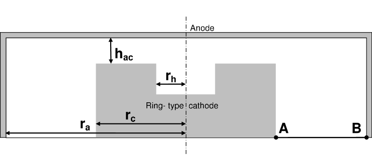
Figure 1: Relativistic vacuum diode with a ring-type cathode

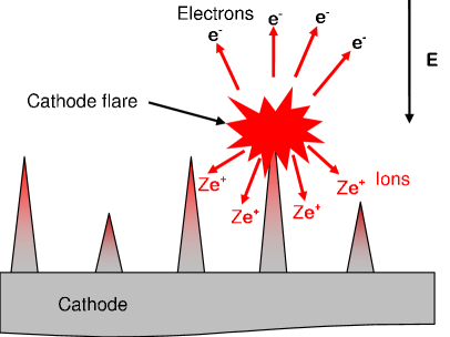
Figure 2: Explosive electron emission

It is noteworthy that $t_{d}$ is particular sensitive to the condition of the cathode surface. It was shown in Farrall1975 that dielectric inclusions on the cathode surface result in the excessive increase of the field-emission current. B.M.Cox and W.T.Williams  Cox1977 reported experimentally observed high electric field strengths near dielectric inclusions on the cathode surface with the local field strength in the vicinity of the inclusions being several hundreds times greater than the average field strength in the cathode-anode gap. The dielectric inclusions, as well as overall surface defects, naturally leads to the time spread $t_{d}$ in the cathode flare formation in different microregions of the cathode.

Dielectric inclusions not only initiate explosive electron emission, but also sustain it  Mesyats1993a . The matter is that the activity of each emitting center is accompanied by the ion flow to the cathode (Fig.2). Dielectric inclusions in the vicinity of the emitting center are charged by the ion current resulting in the breakdown and the formation of new emitting centers. Another mechanism of cathode plasma formation is associated with the field desorption of the atoms absorbed on the cathode surface Litvinov1983 . This occurs in the regions where the local electric field exceeds $\sim 10^{7}$V/cm. Collisional ionization of the desorbed atoms from the field-emission current results in the formation of plasma layer on the cathode surface.

Expansion of the conducting plasma of the cathode flares leads to screening of the nearby regions on the cathode surface by a strong electric field. The analysis given in Mesyats1993c ; Belomytzev1987 ; Belomytzev1980 shows that the characteristic radius of the screened region is

$$r_{scr}\approx 5\cdot 10^{2}\,U^{-3/4}\,i^{1/2}\,h_{ac},$$ (1)

where $U$[V] is the applied voltage, $I$[A] is the cathode flare current, and $h_{ac}$[cm] is the cathode-anode gap. For $U=400$ kV, $i=10$ A, and $h_{ac}=1.5$ cm, the characteristic radius of the screened region, according to (1), is $r_{scr}=0.15$cm.

Thus, the number of the explosive-emission centers $N_{e}$ occurring simultaneously on the surface of the cathode of radius $r_{c}=3$ cm can be estimated at $N_{e}=r_{c}^{2}/r_{scr}^{2}=60$. The number of concurrent explosive-emission centers, $N_{e}$, indicates the degree of inhomogeneity of the beam’s transverse structure.

III Cumulation Mechanism

As it has been stated in the previous section, explosive electron emission begins with the formation and expansion of cathode flares. Explosive electron emission is most intense from the cathode protrusions, particularly from the cathode’s inner edge (Fig.3). Coulomb repulsion causes the charged particles to rush to the region free from the beam. As a result, the accelerated motion of electrons toward the anode comes alongside the radial motion to the cathode’s symmetry axis. As a result, the high-current beam density increases multifold on the axis of the relativistic vacuum diode as compared to the average current density in the cathode-anode gap. The reported cumulation mechanism are described for the ring-type cathode (the circular cathode with a hole, which coincides with the cathode exis). It should be noted that the cumulation mechanism doesn’t depend on the hole position, i.e. whether or not the hole axis coincides with the cathode axis.

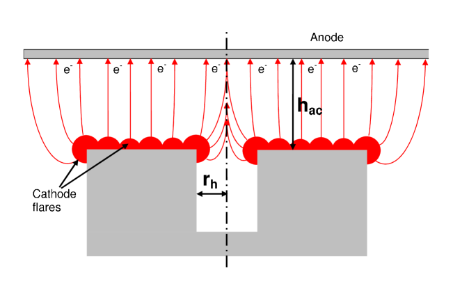
Figure 3: Cumulation caused by electrostatic repulsion

Figure 4 shows the results of simulations: the dose absorbed by the anode. The assumed parameters of the cathode were as follows: cathode radius 3.0 cm, cathode-anode gap 2.0 cm, and the radius of the inner hole 0.8 cm. The maximum value of the accelerating voltage pulse was taken equal to 360 kV and its duration – to 330 ns. The simulated current density in the region of the central spot on the anode at the moment corresponding to the maximum accelerating voltage was as large as 1.0 kA/cm², being 5 times greater than the average current density of the high-current diode. Thus, the simulation result indicate the electron-beam cumulation on the axis of a high-current diode with a ring-type cathode.

The undeniable advantage of this cumulation mechanism over a conventional one based on the self-focusing of a high-current beam by its own magnetic field is a very low energy spread of particles in the region of the maximum current density due to the laminar flow of charged particles (Figure 5). In contrast, under the conditions of self-focusing of the beam by its own magnetic field, the flow current becomes appreciably turbulent, and the charged particles acquire a significant momentum spread Poukey1974 . The electron flow in this case is like a compressed relativistic gas with electron temperature of the order of the voltage applied across the diode Rudakov1990 .

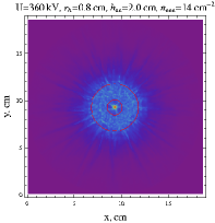
Figure 4: Absorbed dose (simulation results)

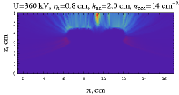
Figure 5: Electron flow (simulation results)

IV Experimental results

To investigate the cathodes and obtain the information about electron beam parameters, we used a nanosecond pulse-periodic electron accelerator with a compact SF6-insulated high-voltage generator (HVG) as a power supply providing pulsed voltage up to 400 kV in $\sim 30$ Ohm resistive load with half-height duration of 130 ns and rise time of 30 ns Bolshakov .

To obtain integrated full-sized imprints of the electron beam, we used a radiochromic dosimetry film (technical specification TU 2379-026-13271746-2006) Generalova placed 3 mm behind the anode mesh made of stainless steel (the geometrical transparency of the mesh was 0.77); the cathode-anode gap was 2 cm. The dosimetry film enabled us to obtain information about the total absorbed dose due to the passage of charged particles Pushkarev2005 .

After the exposure, the transmission scanning of the dosimetry film using the optical filter was made with EPSON Perfection V100 Photo scanner. The distribution of the absorbed dose (and hence the beam’s energy density) over the beam cross section was derived unambiguously from the scanned images and the dose-response calibration curve.

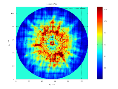
Figure 6: Electron beam imprint without foils

Our first experiments showed that the flow of charged particles on the axis was so intense that it burned the film through (see Fig.6). For this reason, we placed 70 $\mu$m-thick aluminium foils in front of the dosimetry film to decrease the absorbed dose (see Figs. 7–10).

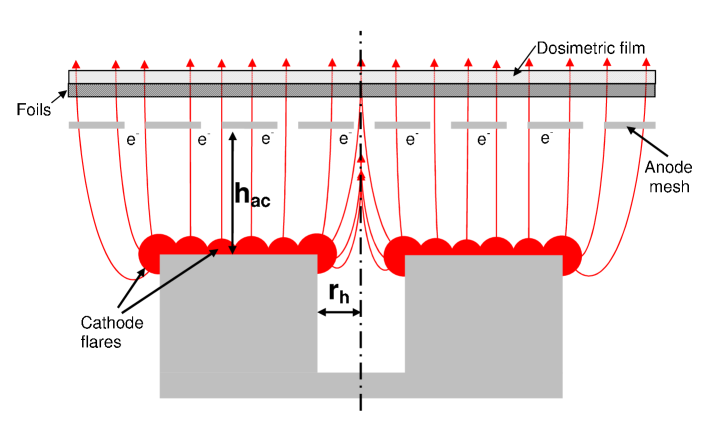
Figure 7: Experimental scheme

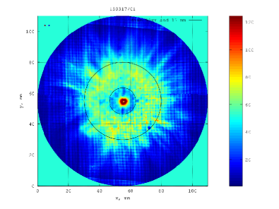
Figure 8: Electron beam imprint with one foil

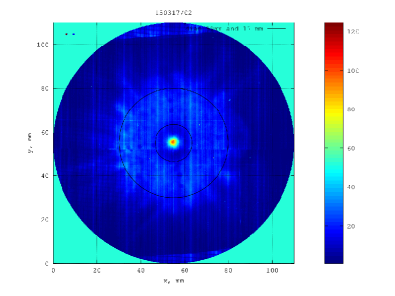
Figure 9: Electron beam imprint with two foils

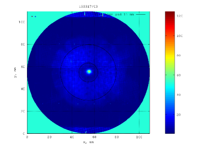
Figure 10: Electron beam imprint with three foils

This enabled us to cut off the flows of both the weakly-relativistic electrons produced at the voltage pulse decay and the cathode plasma. The experiments conducted with one, two, and three foils demonstrated that a sharp increase in the absorbed dose remains in the center. This means that the particle flow consists at the beam axis of high-energy electrons. In the experiments with three foil layers cutting off all electrons whose energy is less than 250 keV, the absorbed dose in the center was almost four times as large as the average dose across the beam cross section, showing a good agreement with the simulation results.

Let us note here that both the simulation and the experiments were performed at maximum accelerating voltage $\sim 400$ kV and the cathode-anode gap equal to 2 cm. The estimates show that with the voltage increased to 2 MV and the cathode-anode gap decreased by a factor of 5 it is possible to achieve the beam intensity of the order of $1$TW/cm² required, for example, to study the extreme states of matter and to do research into inertial confinement fusion.

V Conclusion

In this paper we described the cumulation mechanism of a high-current beam in a relativistic vacuum diode with a ring-type cathode. The basis of this cumulation mechanism is electrostatic repulsion of electrons from the explosive-emission plasma on the inner edge of the cathode. The simulated values of current density and beam intensity equal to $0.36$ GW/cm² and 1 kA/cm², respectively, qualitatively agree with the experimental data.

A very low particle energy spread in the region of maximum current density that is due to laminar flow of charged particle is the distinctive feature of the described cumulation mechanism over a conventional one relying on focusing the high-current beam by its own magnetic field.

Appendix A Simulation of high-current beams

In simulating of the electron beam dynamics under the conditions of nonuniform explosive electron emission, it is necessary to consider the expansion of the cathode plasma emitted from separate explosive emission centers. Self-consistent simulation of particle motion in self- and external electric and magnetic fields is usually performed using the particle-in-cell method Roshal1979 ; Hockney1987 ; Birdsall1989 in a quasi-stationary approximation Poukey1973 ; Golovin1989 . Quasi-stationary approximation applies when the field parameters in high-current diodes change slowly, and the displacement currents and induction fields are neglected.

The simulation is performed in the Cartesian, as well as in cylindrical coordinates. The electric fields and particle motion are computed in the Cartesian coordinate system, while the magnetic fields - in cylindrical. Spatial dimensions of the cells on the mesh for the field calculations are set equal, i.e., $\Delta X=\Delta Y=\Delta Z=\Delta R$. The system is assumed to be axially symmetric, but the numerical simulation of particle motion is performed in 3 dimensions, which is of principal necessity for a proper consideration of the electron emission nonuniformity.

Figure 11: Particle-in-cell

A.1 Particle-in-cell method

The particle-in-cell method has been developed for simulating the multiple phenomena in different fields of physics: vacuum electronics Hartree1941 ; Hartree1950 ; Tien1956 ; Antonsen , plasma physics Buneman1959 ; Lomax1960 ; Birdsall1961 ; Dawson1962 ; Langdon1973 ; Langdon1979 ; Hewitt1987 ; Sveshnikov1989 ; Birdsall1991 ; Verboncoeur2005 , hydrodynamics Harlow1964 , magnetic hydrodynamics Marder1975 ; Brunel1981 , astrophysics Hockney1967 , and semiconductor physics Hockney1974 ; Warriner1976 .

This method consists in the representation of real flows of charged particles (electrons, protons, and ions) as a set of macroparticles, each containing a large number of real charge carriers. Every macroparticle, normally located in a single cell, has a certain attributed spatial distribution of mass and charge. Depending on the charge and the location of the macroparticle, a certain contribution to the charge and current densities is attributed to its nearest nodes on the spatial mesh using the weighting procedure. Using a similar procedure, one can find the forces acting on the macroparticle, knowing the magnitudes of the fields in the nodes located in the close proximity to the particle. Substituting the value for the force into the finite-difference analogues of relativistic equations, we may find new locations and momenta of macroparticles. For a full description of the system of fields and particles, these procedures are completed with charged particle injection into and removal from the computational region.

It is the numerically realized injection of charged particles emitted from the surface of the expanding cathode flares that constitutes the novel and important feature of the developed code.

A typical program cycle based on the particle-in-cell method consists of six operations: computation of coordinates and momenta of particles, injection and removal of particles, computation of the current and charge densities, and computation of the electric and magnetic fields. Now let us proceed to a detailed description of each procedure realized in our code.

A.2 Electric fields

The electric field strength in the quasi-stationary approximation in the Coulomb gauge is related to the scalar potential $\phi$ governed by the Poisson equation:

$$\Delta\phi=-4\pi\rho,$$ (2)

$$\vec{E}=-\nabla\phi.$$ (3)

The analysis given in AG2014 showed that the Jacobi iterative method fits best to solve the Poisson equation for plasma dynamical problems. It is well known Hockney1987 that the iterative methods requiring that the approximate value of the potential at the first iteration step be specified are slowly converging, because the initial distribution usually deviate appreciably from the exact solution of the finite-difference analogue of the Poisson equation. In plasma dynamical problems the situation is basically different, which stems from a more appropriate selection of the initial approximation at the first iteration step: the grid potential magnitudes obtained at the previous time step are taken as the first approximation AG2014 . As a result, the entire iteration process at each time step reduces to one-three iterations, requiring much less time than, say, the computation of new coordinates and positions of the particles.

Thus, with the Jacobi iterative method the final-difference analogue of the Poisson equation has the form:

$$\begin{split}&\frac{\phi_{i+1,j,k}^{n,s}-2\phi_{i,j,k}^{n,s+1}+\phi_{i-1,j,k}^{n,s}}{\Delta X^{2}}+\frac{\phi_{i,j+1,k}^{n,s}-2\phi_{i,j,k}^{n,s+1}+\phi_{i,j-1,k}^{n,s}}{\Delta Y^{2}}\\ &+\frac{\phi_{i,j,k+1}^{n,s}-2\phi_{i,j,k}^{n,s+1}+\phi_{i,j,k-1}^{n,s}}{\Delta Z^{2}}=-4\pi\rho_{i,j,k}^{n},\\ &\phi_{i,j,k}^{n,0}=\phi_{i,j,k}^{n-1},\\ \end{split}$$ (4)

where $s$ is the iteration number and $n$ is the time step number. The iteration in (4) occurs until the residual $|\phi^{n,s}-\phi^{n,s-1}|$ becomes less than $\epsilon|\phi^{n,s}|$. The value of $|\phi^{n,s}|$, which is the norm of the $\phi^{n,s}$ matrix is computed by formula

$$|\phi^{n,s}|=\sqrt{\sum_{i,j,k}(\phi^{n,s}_{i,j,k})^{2}}.$$ (5)

The parameter $\epsilon$ in fact determines the error of the finite-difference Poisson equation solution.

To solve the Poisson equation, we need to complete it with the boundary conditions. We used the Dirichlet boundary condition implying the specified potentials on the cathode ($\phi=U_{c}$) and the anode ($\phi=U_{a}$). At the edge of the computational region in the cathode-anode gap we took the logarithmical distribution of the potential Bugaev1979

$$\phi=U_{c}+\frac{(U_{a}-U_{c})\ln(r/r_{c})}{\ln(r_{a}/r_{c})},$$ (6)

that exactly describes the change in $\phi$ in the gap between two infinite cylinders. Obviously, the distribution of the potential in a high-current diode will approach (8) if the boundary of the computational region stated here is located at a considerable distance from the electron-emitting surface. We shall find the grid density $\rho_{i,j,k}^{n}$ with the linear weighting procedure attributing a certain contribution to $\rho_{i,j,k}^{n}$ coming from eight nodes nearest to the particle located at $(x_{\alpha},y_{\alpha},z_{\alpha})$

$$\begin{split}&\Delta\rho_{i,j,k}^{\alpha n}=q_{\alpha}(1-w^{n}_{i})(1-w^{n}_{j})(1-w^{n}_{k})/\Delta V\\ &\Delta\rho_{i+1,j,k}^{\alpha n}=q_{\alpha}w^{n}_{i}(1-w^{n}_{j})(1-w^{n}_{k})/\Delta V\\ &\Delta\rho_{i,j+1,k}^{\alpha n}=q_{\alpha}(1-w^{n}_{i})w^{n}_{j}(1-w^{n}_{k})/\Delta V\\ &\Delta\rho_{i,j,k+1}^{\alpha n}=q_{\alpha}(1-w^{n}_{i})(1-w^{n}_{j})w^{n}_{k}/\Delta V\\ &\Delta\rho_{i+1,j+1,k}^{\alpha n}=q_{\alpha}w^{n}_{i}w^{n}_{j}(1-w^{n}_{k})/\Delta V\\ &\Delta\rho_{i,j+1,k+1}^{\alpha n}=q_{\alpha}(1-w^{n}_{i})w^{n}_{j}w^{n}_{k}/\Delta V\\ &\Delta\rho_{i+1,j,k+1}^{\alpha n}=q_{\alpha}w^{n}_{i}(1-w^{n}_{j})w^{n}_{k}/\Delta V\\ &\Delta\rho_{i+1,j+1,k+1}^{\alpha n}=q_{\alpha}w^{n}_{i}w^{n}_{j}w^{n}_{k}/\Delta V.\\ \end{split}$$ (7)

Here $\Delta V=\Delta X\Delta Y\Delta Z$ и $\vec{w}^{n}=\Big{(}(x_{\alpha}^{n}-x_{i,j,k})/\Delta X,(y_{\alpha}^{n}-y_{i,j,k})/\Delta Y,(z_{\alpha}^{n}-z_{i,j,k})/\Delta Z\Big{)}$.

After we find the potential, the electric field is found immediately from  Volkov

$$\begin{split}&\vec{E}^{n}_{i,j,k}=-\bigg{(}\frac{\phi^{n}_{i+1,j,k}-\phi^{n}_{i-1,j,k}}{2\Delta X},\frac{\phi^{n}_{i,j+1,k}-\phi^{n}_{i,j-1,k}}{2\Delta Y},\\ &\frac{\phi^{n}_{i,j,k+1}-\phi^{n}_{i,j,k-1}}{2\Delta Z}\bigg{)}.\\ \end{split}$$ (8)

A.3 Magnetic fields

In considering motion of relativistic charged particles, it is fundamentally important to take account of the self- and external magnetic-field effect on the electron-beam dynamics in a high-current diode. As we are concerned with axially symmetric configurations, we shall proceed to cylindrical coordinates. By virtue of axial symmetry, we shall assume that the magnetic field $\vec{H}$ and the current density $\vec{j}$ are independent of the azimuth angle $\theta$.

In the absence of the axial field $H_{z}^{ext}$, $H_{\theta}$ becomes the only magnetic field component and is related to the current density $j_{z}$ and the current $I$ running through the cathode by the Stokes theorem

$$H_{\theta}=\frac{4\pi(I(r,z)+2\pi\int_{0}^{r}j_{z}(r_{1},z)r_{1}dr_{1})}{2\pi cr}.$$ (9)

Here the current $I(r,z)$ contains the contributions coming from all electrons injected into the points with coordinates $>z$.

A.4 Cathode plasma expansion

The center of explosive emission is formed on the cathode when the electric field strength exceeds a certain threshold value $E_{cr}$ that depends on the condition of the electrode surface. Then the cathode flare begins to expand at a speed $v_{eee}\sim 2\cdot 10^{6}$ cm/s in many directions. Without deliberate control over the surface microstructure, the emission centers are chaotically located about the cathode surface. The mean distance between them is determined by the size of the screened area $d_{scr}=2r_{scr}\sim 3$ mm (see (1)), knowing which we can easily estimate the characteristic density $n_{eee}$ of the explosive-emission centers $n_{eee}=1/\pi r_{scr}^{2}\sim 14$ cm^-2.

For the purposes of high-current diodes simulation, we shall assume that the emission regions are formed in the cathode nodes where the electric field exceeds $E_{cr}$ with the probability $n_{eee}(\Delta X\Delta Y\Delta Z)^{2/3}$. When the electric field becomes greater than $E_{cr}$, the cathode flare expands at a constant speed $v_{eee}$ in every direction from the emission region. Each cathode flare is the source of electrons. The active cathode flare emits thermionic emission current which is many times as large as the current limited by the beam space charge, and so we can speak about the unlimited thermionic emission resulting in practically zero field on the surface of the expanding cathode plasma. The assumption about the cathode screening enables us to appreciably simplify the numerical computation of the charged-particle kinetics, sparing ourselves the need to simulate fast processes just in the emission region. Such simulation would require a high space-time resolution due to the smallness of the Debye length and high values of plasma oscillation frequency AG2014 .

At each time step, we inject the charged particles into plasma-occupied nodes that have in the vicinity at least one node free from the conducting material. The magnitude of the injected charge $Q_{i,j,k}$ is found from the relation

$$\begin{split}&Q_{i,j,k}=\Big{(}\frac{E_{xi+1,j,k}^{n}-E_{xi-1,j,k}^{n}}{2\Delta X}+\frac{E_{xi,j+1,k}^{n}-E_{xi,j-1,k}^{n}}{2\Delta Y}\\ &+\frac{E_{xi,j,k+1}^{n}-E_{xi,j,k-1}^{n}}{2\Delta Z}\Big{)}\frac{\Delta X\Delta Y\Delta Z}{4\pi}.\\ \end{split}$$ (10)

Let us note that the charge is injected if $Q_{i,j,k}<0$.

A.5 Motion of charged particles

Numerical integration of relativistic equations of motion is the most time-consuming procedure of all, that is why it is paid special attention to by the developers of the codes. In a nonrelativistic case, the most widely used is the leapfrog scheme Birdsall1989 ; Verboncoeur2005

$$\begin{split}&\vec{p}_{\alpha}^{n+1/2}=\vec{p}_{\alpha}^{n-1/2}+\vec{F}_{\alpha}^{n}\Delta T,\\ &\vec{r}_{\alpha}^{n+1}=\vec{r}_{\alpha}^{n}+\frac{\vec{p}_{\alpha}^{n+1/2}}{m_{\alpha}}\Delta T,\\ \end{split}$$ (11)

Because the magnetic fields may be neglected, the forces $\vec{F}_{\alpha}^{n}=q_{\alpha}\vec{E}_{\alpha}^{n}$ contain only the electric field, their magnitudes being unambiguously defined by the positions of particles and boundary conditions. In the relativistic case, the scheme (11) cannot be used directly, because $\vec{F}_{\alpha}^{n}$ includes the Lorentz force $q_{\alpha}\vec{v}_{\alpha}^{n}\times\vec{H}_{\alpha}^{n}$, depending on the velocity $\vec{v}_{n}$ determined at time $T_{n}=n\Delta T$. However, in the leapfrog scheme, the particle velocities are defined at half-integral times $T_{n+1/2}=(n+1/2)\Delta T$. The natural solution allowing us to retain the simplicity of the leapfrog scheme in this situation is the application of Lagrange’s interpolation formula for computing $\vec{v}_{\alpha}^{n+1}$ from the three values of the velocity ($\vec{v}_{\alpha}^{n-3/2}$, $\vec{v}_{\alpha}^{n-1/2}$, $\vec{v}_{\alpha}^{n+1/2}$)

$$\vec{v}_{\alpha}^{n+1}=\frac{3\vec{v}_{\alpha}^{n-3/2}-10\vec{v}_{\alpha}^{n-1/2}+15\vec{v}_{\alpha}^{n+1/2}}{8}.$$ (12)

Thus, the complete integration scheme of the equations of motion takes the form:

$$\begin{split}&\vec{p}_{\alpha}^{n+1/2}=\vec{p}_{\alpha}^{n-1/2}+q_{\alpha}(\vec{E}_{\alpha}^{n}+\vec{v}_{\alpha}^{n}\times\vec{H}_{\alpha}^{n})\Delta T,\\ &\vec{v}_{\alpha}^{n+1/2}=\frac{c\vec{p}_{\alpha}^{n+1/2}}{\sqrt{m_{\alpha}^{2}c^{2}+(\vec{p}_{\alpha}^{n+1/2})^{2}}}\\ &\vec{r}_{\alpha}^{n+1}=\vec{r}_{\alpha}^{n}+\vec{v}_{\alpha}^{n+1/2}\Delta T,\\ &\vec{v}_{\alpha}^{n+1}=\frac{3\vec{v}_{\alpha}^{n-3/2}-10\vec{v}_{\alpha}^{n-1/2}+15\vec{v}_{\alpha}^{n+1/2}}{8}.\\ \end{split}$$ (13)

The fields $\vec{E}_{\alpha}^{n}$ and $\vec{H}_{\alpha}^{n}$ acting on the particle are determined from the magnitudes of the mesh fields in the eight adjacent nodes Verboncoeur2005 :

$$\begin{split}&\vec{E}_{\alpha}^{n}=\vec{E}_{i,j,k}^{n}(1-w^{n}_{i})(1-w^{n}_{j})(1-w^{n}_{k})\\ &+\vec{E}_{i+1,j,k}^{n}w^{n}_{i}(1-w^{n}_{j})(1-w^{n}_{k})\\ &+\vec{E}_{i,j+1,k}^{n}(1-w^{n}_{i})w^{n}_{j}(1-w^{n}_{k})\\ &+\vec{E}_{i,j,k+1}^{n}(1-w^{n}_{i})(1-w^{n}_{j})w^{n}_{k}\\ &+\vec{E}_{i+1,j+1,k}^{n}w^{n}_{i}w^{n}_{j}(1-w^{n}_{k})\\ &+\vec{E}_{i,j+1,k+1}^{n}(1-w^{n}_{i})w^{n}_{j}w^{n}_{k}\\ &+\vec{E}_{i+1,j,k+1}^{n}w^{n}_{i}(1-w^{n}_{j})w^{n}_{k}\\ &+\vec{E}_{i+1,j+1,k+1}^{n}w^{n}_{i}w^{n}_{j}w^{n}_{k}.\\ \end{split}$$ (14)

References

- (1) W.H. Bennet, Phys. Rev. 1934. 45. 890–897.
- (2) H. Alfven, Phys. Rev. 1939. Vol. 55. No. 5. P. 425–429.
- (3) S.E. Graybill, S.V. Nablo, IEEE Trans. Nucl. Sci. 1967. P. 782–788.
- (4) W.T. Link, IEEE Trans. Nucl. Sci. 1967. P. 777–781.
- (5) F.M. Charbonnier, et. al., IEEE Trans. Nucl. Sci. 1967. P. 789–793.
- (6) S.E. Graybill, IEEE Trans. Nucl. Sci. 1971. P. 438–446.
- (7) I.O. Shipman, IEEE Trans. Nucl. Sci. 1971. P. 243–246.
- (8) W.P. Dyke, J.K. Trolan, E.E. Martin, J.P. Barbour, Phys. Rev. 1953. Vol. 91. P. 1043–1054.
- (9) W.W. Dolan, W.P. Dyke, J.K. Trolan, Phys. Rev. 1953. Vol. 91. P. 1054–1057.
- (10) J.C. Martin, Proceedings of the IEEE. 1992. Vol. 80. P. 934–945.
- (11) D.L. Morrov, J.D. Phillips, W.H. Bennett, et. al. J. Appl. Phys. 1971. Vol. 19. P. 441–443.
- (12) L.P. Bradley, G.W. Kuswa, Phys. Rev. Lett. 1972. Vol. 29. P. 1441–1445.
- (13) G. Yonas, Presented at the IV National School on Plasma Physics, Novosibirsk, USSR, 1974.
- (14) L.I. Rudakov, A.A. Samarsky, Proc. 6th European Conf. on Controlled Fusion and Plasma Phys., Moscow, July 1974. P. 487.
- (15) A.C. Kolb, IEEE Trans. Nucl. Sci. 1967. P. 956–961.
- (16) G. Yonas, Sci. American 1978. Vol. 239. No. 5. P. 40–51.
- (17) G.A. Mesyats, Pulsed Power Berlin Springer 2005.
- (18) T.H. Martin, IEEE Trans. Nucl. Sci. 1969. P. 59–63.
- (19) N.F. Kovalev and et. al, JETP Lett. 1973. Vol. 18. P. 232–235.
- (20) Y. Carmel, J. Ivers, R.E. Kribel, J. Nation, Phys. Rev. Lett. 1974. Vol. 33. P. 1278–1282.
- (21) J. Rander, B. Ecker, G. Yonas, D.J. Drickey, Phys. Rev. Lett. 1970. Vol. 24. P. 283–286.
- (22) A.E. Dubinov, I.Ju. Kornilova, V.D. Selemir, Phys. Usp. 2002. Vol. 172. P. 1109–1129.
- (23) N.G. Basov, V.A. Danilychev, Sov. Phys. Usp. 1986. Vol. 29. P. 31–56.
- (24) S.V. Anishchenko, A.A. Gurinovich, EAPPC 2014, Kumamoto, Japan.
- (25) G.A. Mesyats, D.I. Proskurovsky, JETP Lett. Vol. 13. P. 7–10.
- (26) S.P. Bugaev, E.A. Litvinov, G.A. Mesyats, D.I. Proskurovskii, Sov. Phys. Usp. 1975. Vol. 18. P. 51–61.
- (27) G.A. Mesyats, Plasma Phys. Control. Fusion 47 (2005) A109-A151.
- (28) R.W. Wood, Phys. Rev. 1897. Vol. 5. P. 1.
- (29) R.H. Fowler, L. Nordheim, Roy. Soc. Proc. 1928. 119A. P. 173–181.
- (30) R.A. Millikan, C.C. Lauritsen, Phys. Rev. 1929. Vol. 33. P. 598.
- (31) E.L. Murphy, R.H. Good, Phys. Rev. 1956. Vol. 102. P. 1464–1473.
- (32) G.A. Farrall, M. Owens, F.G. Hudda, J. Appl. Phys. 1975. Vol. 46. P. 610—617
- (33) B.M.Cox, W.T.Williams: J. Phys. D10, L5–9 (1977).
- (34) G.A. Mesyats. Ectons. Part 1. Ekaterenburg: UIF «Nauka», 1993.
- (35) E.A. Litvinov, G.A. Mesyats, D.I. Proskurovsky, Sov. Phys. Usp. 1983. Vol. 26. P. 138–159.
- (36) G.A. Mesyats. Ectony. Chast 3. Ekaterenburg: UIF «Nauka», 1993.
- (37) S.Ja. Belomytzev, G.A. Mesyats, Radioelectronica. 1987. Vol. 32. P. 1569–1583.
- (38) S.Ja. Belomytzev, S.D. Korovin, G.A. Mesyats, JTP Lett. 1980. Vol. 6. P. 1089–1092.
- (39) J.W. Poukey, A.J. Toepfer, Phys. Fluids. 1974. Vol. 17. P. 1582–1591.
- (40) E.P.Bolshakov et. al. // VANT, Ser “Electrofizicheskaya apparatura” vyp. 5(13), 2010, P. 137-147.
- (41) V.V. Generalova, M.N. Gursky. Dozimetriya v radiacionnoj tehnologii. - M.: Izdatelstvo standartov, 1981.
- (42) D.V. Goncharov et. al. Izv. Tomskogo politehnicheskogo universiteta, 2005, Vol. 308, No. 6, P. 76-80.
- (43) A.S. Roshal, Modelirovanie zarjazhennyh puchkov. —M.: Atomizdat, 1979.
- (44) R.W. Hockney, J.W. Easwood, Computer simulation using particles, McGraw-Hill, New York 1981.
- (45) C.K. Birdsall, A.B. Langdon, Plasma physics via computer simulation: McGraw-Hill, New York 1985.
- (46) J.W. Poukey, J.R. Freeman, G. Yonas, J. Vac. Sci. Technol. 1973. Vol. 10. No. 6. P. 954–958.
- (47) G.T. Golovin, Zh. vychisl. matem. i matem. fiz. 1989. Vol. 29. P. 423–437. University, 1976.
- (48) D.R. Hartree, P. Nicolson, CVD Reports Mag. 3, 12, 18, 23, 36, British Admiralty, London (1941–1944).
- (49) D.R. Hartree, Appl. Sci. Res. Col. B1, P. 379–390.
- (50) P.K. Tien, J. Moshman, J. Appl. Phys. 1956. Vol. 27. P. 1067–1078.
- (51) T. M. Antonsen, et. al. Proceedings of the IEEE. 1999. Vo. 87. P. 804.
- (52) O. Buneman, Phys. Rev. 1959. Vol. 115. P. 503–517.
- (53) R.J. Lomax, J. Electron & Control. 1960. Vol. 9. P. 127–140.
- (54) C.K. Birdsall, W.B. Bridges, J. Appl. Phys. Vol. 32. P. 2611–2618.
- (55) J.M. Dawson, Phys. Fluids. 1962. Vol. 5. P. 445–459.
- (56) A.B. Langdon, J. Comput. Phys. 1973. Vol. 12. P. 247–268.
- (57) A.B. Langdon, Phys. Fluids, 1979. Vol. 22. P. 163–171.
- (58) D.W. Hewitt, A.B. Langdon, J. Comput. Phys. 1987. Vol. 72. P. 121.
- (59) A. G. Sveshnikov, S. A. Jakunin, Matematicheskoe modelirovanie. 1989. Vol. 1. No. 4. P. 1.
- (60) C. K. Birdsall, IEEE Trans. Plasma Sci. 1991. Vol. 19. No. 2. P. 65.
- (61) J. P. Verboncoeur, Plasma Phys. Control. Fusion. 2005. Vol. 47. P. 231.
- (62) F. H. Harlow, Methods Comput. Phys. 1964. Vol. 3. P. 319–343.
- (63) R.M. Marder, Math. Comput. 1975. Vol. 29. P. 434–446.
- (64) F. Brunel, et al. J. Comput. Phys. 43. 268 (1981).
- (65) R.W. Hockney, Astrophys. J. 1967. Vol. 150. P. 797–806.
- (66) R.W. Hockney, R.A. Warrier, M. Reiser, Electron. Lett. 1974. Vol. 10. P. 484–486.
- (67) R.A. Warriner, Computer Simulation of Gallium Arsenide Semiconductor Devices, Ph.D. Thesis, Reading University, 1976.
- (68) B. Marder, J. Comp. Phys. 1987. Vol. 68. P. 48–55.
- (69) S.V. Anishchenko, A.A. Gurinovich, Computational Science & Discovery. 2014. Vol. 7. P. 015007.
- (70) E.A. Volkov, Numerical methods. Moscow: Science, 1987.
- (71) S.P. Bugaev et al. in: Relyativistskaya vakuumnaya electronika. Gorky: 1979. P. 5–75.