Exponential bound on information spreading induced by quantum many-body dynamics with long-range interactions

Abstract

The dynamics of quantum systems strongly depends on the local structure of the Hamiltonian. For short-range interacting systems, the well-known Lieb-Robinson bound defines the effective light cone with an exponentially small error with respect to the spatial distance, whereas we can obtain only polynomially small error for distance in long-range interacting systems. In this paper, we derive a qualitatively new bound for quantum dynamics by considering how many spins can correlate with each other after time evolution. Our bound characterizes the number of spins which support the many-body entanglement with exponentially small error and is valid for large class of Hamiltonians including long-range interacting systems. To demonstrate the advantage of our approach in quantum many-body systems, we apply our bound to prove several fundamental properties which have not be derived from the Lieb-Robinson bound.

1 Introduction

The fundamental features of quantum many-body systems are strongly restricted by the local nature of Hamiltonian. Such restrictions give us a lot of useful information in analyzing universal properties of matters. One of the prominent examples is the Lieb-Robinson bound [1, 2], which characterizes the velocity of information propagation in non-relativistic quantum systems; in other words, we can define an approximate “light cone” with an exponentially small error. Based on the Lieb-Robinson bound, we can grasp fundamental restrictions to quantum dynamics: entropy production rate after quench [3, 4, 5, 6], entanglement growth [7, 8, 9, 10, 11, 12, 13, 14], complexity of quantum simulation [15, 16, 17, 18, 19], and so on. Moreover, the Lieb-Robinson bound also provides us powerful analytical tools to give foundations of quantum many-body systems, from condensed matter physics to statistical mechanics: Lieb-Schultz-Mattis theorem [20, 21], exponential decay of bi-partite correlation [22, 23, 24], stability of topological order to perturbation [25, 26, 2, 27, 28], quantization of the Hall conductance [29, 30], thermalization problem [31, 32], equivalence of the statistical ensembles [33], etc. In these results, the locality of interactions plays essential roles. Thus, the principle of locality has shed new light on our understanding of fundamental many-body physics.

More recently, with the progress of experimental technology [34, 35, 36, 37], there has been considerable interest in the potential of the locality analysis in long-range interacting systems, both from theoretical [38, 39, 40, 9, 41, 42, 43, 44, 45, 46, 47] and experimental [36, 37] viewpoints. In such systems, we can also define the approximate light cone as in the case of the short-range interacting systems. However, the light-cone is usually nonlinear to the time except some special cases [42], and moreover the transport of information can be bounded only polynomially [41, 46, 23, 36, 42] with respect to the spatial distance outside the light cone. The primary reason is that the Lieb-Robinson bound focuses on the velocity of the information transfer, whereas the long-range interacting systems can transport information immediately in principle. In this way, the causality allows us to analyze the system in the looser way in comparison with the case of the short-range interacting systems. This indicates that we may not grasp all the restrictions due to the locality of the Hamiltonian in terms of only the spatial distance. Here, we use the term of “locality” in more broader meanings [40] as distinguished from the spatial locality, i.e., to what extent can quantum systems be described by a collection of local degrees of freedom, which are only loosely correlated with each other?

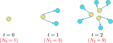
Figure 1: Schematic picture of classical information spreading. We consider a classical system with $N$ elements and assume that each of the elements is connected to arbitrary ones. We start from one information source (e.g., coded by $0$ or $1$) and consider the process that each element which has received the information can send the information to other $2$ elements per unit of time. For example, after a unit of time, $2$ elements receive the information and then totally $3$ elements becomes the next information source. In the same way, after two units of time, totally $9$ elements share the information. Repeatedly, the number of receivers　 after $n$ units of time, say $N_{n}$, increases as $3^{n}$. By analogy, we also expect that the information spreading of spins should be similarly suppressed in the quantum many-body dynamics.

In the present paper, we give a qualitatively new bound for dynamical properties in terms of the number of spins instead of the spin-spin distance; roughly speaking, we focus on how many spins can correlate with each other after time evolution. In order to make our concept clear, we first consider a classical process in which a source transfers information to receivers. We now assume that each of the elements sends information to any other 2 elements per unit of time (see Fig. 1). Then, the number of elements which share the information can be bounded from above by $e^{\mathcal{O}(t)}$. Our main purpose is to give a quantum version of the bound in the form of an operator inequality. As we shall see shortly, our new bound characterizes the number of particles which support many-body entanglement such as the topological order [2] and the macroscopic entanglement [48, 49]; this indicates that the global entanglement induced by a small-time evolution should be suppressed up to exponentially small error. It allows us to obtain novel strong properties on various kinds of fundamental physics in quantum many-body systems which have not be derived from the Lieb-Robinson bound.

2 Model and formalism

We consider a spin system of finite volume with each spin having a $d$-dimensional Hilbert space and label each spin by $i=1,2,\ldots N$.　 We denote the set of all spins by $\Lambda:=\{1,2,\ldots,N\}$ We denote partial sets of sites by $X$, $Y$, $Z$ and so on and the cardinality of $X$, that is, the number of sites contained in $X$, by $|X|$ (e.g. $X=\{i_{1},i_{2},\ldots,i_{|X|}\}$). We here define the $q$-local operator $\Gamma^{(q)}$ as follows:

$$\Gamma^{(q)}=\sum_{|X|\leq q}\gamma_{X}\quad\textrm{($q$-locality)},$$ (1)

where each of the $\{\gamma_{X}\}$ is supported in a finite set $X\subset\Lambda$. In other words, the $q$-local operator contains up to $q$-body coupling.

Here, we assume systems which are governed by $k$-local Hamiltonians with $k=\mathcal{O}(1)$:

$$H=\sum_{|X|\leq k}h_{X}.$$ (2)

We assume the time-independence of the Hamiltonian for the simplicity, but the discussion can be generalized to the time-dependent Hamiltonian $H(t)$. Note that we make no assumption on the geometry of the system, and the coupling can be arbitrarily long ranged. Instead, as a normalization factor, we introduce the parameter $g$ of the Hamiltonian:

$$\sum_{X:X\ni i}\|h_{X}\|\leq g\quad{\rm for}\quad\forall i\in\Lambda\quad\textrm{($g$-extensiveness)}$$ (3)

with $\|\cdots\|$ the operator norm (i.e., the maximum singular value of the operator); we refer to that the Hamiltonian is $g$-extensive if it satisfies the condition (3). This implies that the energy associated with one spin is bounded by a finite value $g$. Note that the norm of the Hamiltonian $\|H\|$ increases at most linearly with the system size $N$, namely

$$\|H\|=\left\|\sum_{X}h_{X}\right\|\leq\sum_{X}\|h_{X}\|\leq\sum_{i=1}^{N}\sum_{X:X\ni i}\|h_{X}\|\leq\sum_{i=1}^{N}g=gN.$$ (4)

We notice that the class of $k$-local Hamiltonians covers almost all realistic quantum many-body systems not only with short-range interactions but also with long-range interactions.

For the basic analysis of the $k$-local Hamiltonian, we utilize the following theorem:

Theorem 2.1

Let $H$ be a $k$-local $g$-extensive Hamiltonian and $\Gamma^{(q)}$ be a $q$-local operator; note that the $\Gamma^{(q)}$ may not be extensive as in (3). Then, for an arbitrary positive integer $q$, we can obtain

$$\|[H,\Gamma^{(q)}]\|\leq\lambda\frac{q}{k}\|\Gamma^{(q)}\|\quad{\rm with}\quad\lambda:=6gk^{2}.$$ (5)

Note that the operator $[H,\Gamma^{(q)}]$ is still at most $(k+q)$-local. In the case where $\Gamma^{(q)}$ is supported in a local subset $Z\subset\Lambda$, namely $\Gamma^{(q)}=\gamma_{Z}$ ($|Z|=q$), we can simply prove the theorem as follows:

$$\|[H,\gamma_{Z}]\|\leq\sum_{X:X\cap Z\neq\emptyset}\|[h_{X},\gamma_{Z}]\|\leq\sum_{i\in Z}\sum_{X:X\ni i}2\|h_{X}\|\cdot\|\gamma_{Z}\|\leq 2g|Z|\cdot\|\gamma_{Z}\|\leq 6gqk\|\gamma_{Z}\|.$$ (6)

When $\Gamma^{(q)}$ is a general $q$-local operator, however, the proof cannot be given in a simple way but a bit technical. To show the point, we expand a $q$-local operator $\Gamma^{(q)}$ as

$$\Gamma^{(q)}=\sum_{|Z|\leq q}\gamma_{Z}.$$

Now, the difficulty lies in the fact that we cannot utilize the following simple estimation; we have

$$\|[H,\Gamma^{(q)}]\|\leq\sum_{|Z|\leq q}\|[H,\gamma_{Z}]\|\leq 2gq\sum_{|Z|\leq q}\|\gamma_{Z}\|,$$

whereas we cannot generally ensure

$$\sum_{|Z|\leq q}\|\gamma_{Z}\|\propto\|\Gamma^{(q)}\|.$$

For example, let us consider the following $2$-local operator

$$\Gamma^{(2)}=\frac{1}{N}\sum_{i<j}\gamma_{i,j}\sigma_{i}^{z}\otimes\sigma_{j}^{z},$$

where $\{\gamma_{i,j}\}_{i,j=1}^{N}$ are uniform random numbers from $-1$ to $1$. For this operator, we can obtain $\sum_{i<j}\|\gamma_{i,j}\sigma_{i}^{z}\otimes\sigma_{j}^{z}\|/N=\mathcal{O}(N)$, but $\|\Gamma^{(2)}\|=\mathcal{O}(\sqrt{N})$, and hence

$$\|[H,\Gamma^{(2)}]\| \leq\sum_{|Z|\leq 2}\|[H,\gamma_{Z}]\|\leq 4g\sum_{i<j}\frac{\|\gamma_{i,j}\sigma_{i}^{z}\otimes\sigma_{j}^{z}\|}{N}=4g\mathcal{O}(\sqrt{N})\|\Gamma^{(2)}\|,$$

where the second inequality comes from (6). This is much looser than the inequality (5) which comes from Theorem 2.1. We give the full proof in A.

3 Main results

In order to mathematically apply the classical discussion on the information sharing to quantum cases, we consider the dynamics of the $k$-locality of operators. We initially consider a $q_{0}$-local operator $\Gamma^{(q_{0})}$ and investigate its time evolution: $\Gamma^{(q_{0})}(t)=e^{-iHt}\Gamma^{(q_{0})}e^{iHt}.$ After a time evolution, the operator $\Gamma^{(q_{0})}(t)$ will be no longer a $q_{0}$-local operator but may be approximated by another $q$-local operator with $q\geq q_{0}$, say $\Gamma_{t}^{(q)}$. We now regard $q_{0}$ and $q$ as the numbers of particles which share the information at the times $0$ and $t$ as in Fig. 1, respectively. We then expect that the approximation can be rapidly improved beyond $q\gtrsim q_{0}e^{\mathcal{O}(t_{0})}$ from the classical discussion. Indeed, we prove the following theorem for the minimal error of the approximation:

Theorem 3.1

Let $\mathcal{U}(q)$ be a set of $q$-local operators and consider an arbitrary $q_{0}$-local operator $\Gamma^{(q_{0})}\in\mathcal{U}(q_{0})$. Then, for an arbitrary real-time evolution with $t>0$, there exists a $q$-local operator $\Gamma_{t}^{(q)}$ which approximates the operator $\Gamma^{(q_{0})}(t)$ with the following error:

$$\inf_{\Gamma_{t}^{(q)}\in\mathcal{U}(q)}\bigl{(}\|\Gamma^{(q_{0})}(t)-\Gamma_{t}^{(q)}\|\bigr{)}\leq 8\|\Gamma^{(q_{0})}\|\lceil\kappa t\rceil\exp\biggl{[}-\frac{1}{\xi}\Bigl{(}\frac{q}{r_{t}}-q_{0}\Bigr{)}\biggr{]}$$ (7)

with $\kappa=4\lambda$, $\xi=k/\log 2$ and $r_{t}=2^{\lceil\kappa t\rceil}-1$, where $\lceil\cdots\rceil$ denotes the ceiling function. The same inequality holds for $t<0$ by replacing $t$ with $|t|$.

Because the function $r_{t}$ increases as $e^{\mathcal{O}(t)}$, the time-evolution of $\Gamma^{(q_{0})}$ can be well approximated by a $(q_{0}e^{\mathcal{O}(t)})$-local operator. The upper bound is meaningful as long as $t\lesssim\log N$, which is qualitatively consistent with the threshold time of the breakdown of the Lieb-Robinson bound for long-range interacting Hamiltonians. As in the case of the Lieb-Robinson bound [41, 42], we might improve the present theorem by explicitly considering a spatial structure of the system, for example, the power-law decay of interaction.

We also mention the case where the system is governed by a short-range interacting Hamiltonian. In this case, we can obtain much stronger restrictions [2]. Let us consider an operator $\Gamma_{L}$ which is supported in a region $L$. After a short time, the operator $\Gamma_{L}(t)$ is no longer supported in the region $L$, but is approximately supported in some region having distance $l$ from $L$. The Lieb-Robinson bound ensure that the accuracy of this approximation becomes precise exponentially as the distance $l$ increases beyond $\mathcal{O}(t)$. In other words, the support of $\Gamma_{L}(t)$ enlarges at most as ${\rm Poly}(t)$ instead of $e^{\mathcal{O}(t)}$.

Proof of Theorem 3.1. For the proof, we first obtain the upper bound for a small-time evolution:

$$\inf_{\Gamma_{t}^{(q)}\in\mathcal{U}(q)}\bigl{(}\|\Gamma^{(q_{0})}(t)-\Gamma_{t}^{(q)}\|\bigr{)}\leq 2^{q_{0}/k}\cdot\frac{(\kappa t/2)^{(q-q_{0})/k}}{1-\kappa t/2}\|\Gamma^{(q_{0})}\|$$ (8)

for $t<2/\kappa$. In the derivation of (8), we use the direct expansion of $e^{-iHt}\Gamma^{(q_{0})}e^{iHt}$ according to the Hadamard lemma of the form

$$\Gamma^{(q_{0})}(t)=\sum_{m=0}^{\infty}\frac{(-it)^{m}}{m!}\overbrace{[H,[H,\cdots[H}^{m},\Gamma^{(q_{0})}]]\cdots].$$ (9)

We terminate the expansion (9) at $m=m_{0}$ so that the expanded operator may be $q$-local. We then estimate the error due to the termination to prove the bound (8). We show the full proof in B.

We, however, cannot utilize the expansion (9) in order to obtain a meaningful bound for $t>2/\kappa$. In obtaining the inequality (7), we will have to utilize the fact that $e^{-iHt}$ is unitary . For this purpose, we split the time range $[0,t]$ into $n$ intervals (Fig. 2) such that $t/n\leq 1/\kappa$. We here denote the length of the interval $t/n$ by $\delta t$:

$$\delta t:=\frac{t}{n}\leq\frac{1}{\kappa}\quad{\rm with}\quad n:=\lceil\kappa t\rceil.$$ (10)

We also define $t_{m}:=m\delta t$ for $m=0,1,2,\ldots n$ with $t_{n}=t$. Note that in each interval we can now apply the upper bound (8).

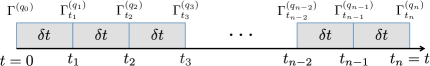
Figure 2: Schematic picture of the proof of Theorem 3.1. For small-time evolutions, we can obtain the approximation of $\Gamma^{(q_{0})}(t)$ directly by the use of the time expansion as in Eq. (9). For long-time evolutions, we split the total time range $[0,t]$ into $n$ intervals with a length $\delta t$. In each of the intervals, we can apply the result for small-time evolutions, and hence we can connect the approximations as follows; we first approximate $\Gamma^{(q_{0})}(\delta t)$ by $\Gamma^{(q_{1})}_{t_{1}}$, second approximate $\Gamma^{(q_{1})}_{t_{1}}(\delta t)$ by $\Gamma^{(q_{2})}_{t_{2}}$ and so on. Then, we can finally prove that the operator $\Gamma^{(q_{n})}_{t_{n}}$ satisfies the inequality (7) by choosing the set $\{q_{m},\Gamma^{(q_{m})}_{t_{m}}\}_{m=1}^{n}$ appropriately.

In the following, we connect the approximations of $\Gamma^{(q_{0})}(t)$ from the first interval $[0,t_{1})$ to the last interval $[t_{n-1},t_{n}]$. We first approximate the time evolution $\Gamma^{(q_{0})}(\delta t)$ with a $q_{1}$-local operator $\Gamma^{(q_{1})}_{t_{1}}$. We second approximate $\Gamma^{(q_{1})}_{t_{1}}(\delta t)$ with a $q_{2}$-local operator $\Gamma^{(q_{2})}_{t_{2}}$. By sequentially repeating this process, we define a set of operators $\{\Gamma^{(q_{m})}_{t_{m}}\}_{m=1}^{n}$ so that they may approximately satisfy $\|\Gamma^{(q_{m})}_{t_{m}}(\delta t)-\Gamma^{(q_{m+1})}_{t_{m+1}}\|\simeq 0,$ respectively, where $q_{n}\leq q$. We thus obtain the approximation of $\Gamma^{(q_{0})}(t)$ by the use of the set $\{\Gamma^{(q_{m})}_{t_{m}}\}_{m=1}^{n}$:

$$\|\Gamma^{(q_{n})}_{t_{n}}-\Gamma^{(q_{0})}(t)\|$$

$$= \biggl{\|}\sum_{m=1}^{n}\bigl{[}\Gamma^{(q_{m})}_{t_{m}}(t_{n}-t_{m})-\Gamma^{(q_{m-1})}_{t_{m-1}}(t_{n}-t_{m}+\delta t)\bigr{]}\biggr{\|}$$

$$\leq \sum_{m=1}^{n}\bigl{\|}\Gamma^{(q_{m})}_{t_{m}}(t_{n}-t_{m})-\Gamma^{(q_{m-1})}_{t_{m-1}}(t_{n}-t_{m}+\delta t)\bigr{\|}$$

$$= \sum_{m=1}^{n}\bigl{\|}\Gamma^{(q_{m})}_{t_{m}}-\Gamma^{(q_{m-1})}_{t_{m-1}}(\delta t)\bigr{\|},$$ (11)

where we used the equality $t_{m+1}-t_{m}=\delta t$ in the first line, the norm invariance during the time evolution in the third line, and we set $\Gamma^{(q_{0})}_{t_{0}}=:\Gamma^{(q_{0})}$. Note that we use the unitarity of the time evolution in the third equality.

We can then show the appropriate choice of the set $\{q_{m},\Gamma^{(q_{m})}_{t_{m}}\}_{m=1}^{n}$. From the inequality (8), we can prove that there exists a set $\{q_{m},\Gamma^{(q_{m})}_{t_{m}}\}_{m=1}^{n}$ such that:

$$\bigl{\|}\Gamma^{(q_{m})}_{t_{m}}-\Gamma^{(q_{m-1})}_{t_{m-1}}(\delta t)\bigr{\|}\leq\Delta(\Delta+1)^{m-1}\|\Gamma^{(q_{0})}\|$$ (12)

for $m=1,2,\ldots,n$, respectively, with $\Delta:=4\exp\bigl{[}-\frac{1}{\xi}\Bigl{(}\frac{q}{r_{t}}-q_{0}\Bigr{)}\bigr{]}$. The derivation is given in C.

By combining the inequalities (11) and (12), we have

$$\|\Gamma^{(q_{n})}_{t_{n}}-\Gamma^{(q_{0})}(t)\| \leq\sum_{m=1}^{n}\Delta(\Delta+1)^{m-1}\|\Gamma^{(q_{0})}\|$$ (13)

$$=\bigl{[}(\Delta+1)^{n}-1\bigr{]}\cdot\|\Gamma^{(q_{0})}\|.$$

We can always find an operator $\Gamma^{(q_{n})}_{t_{n}}$ such that $\|\Gamma^{(q_{n})}_{t_{n}}-\Gamma^{(q_{0})}(t)\|\leq\|\Gamma^{(q_{0})}\|$ (e.g. $\Gamma^{(q_{n})}_{t_{n}}=0$), and hence we only have to consider the range $(\Delta+1)^{n}-1\leq 1$ in the above inequality and obtain 

$$(\Delta+1)^{n}-1\leq 2^{1-1/n}\cdot n\cdot\Delta<2n\Delta.$$ (14)

The inequality (13) reduces to the inequality (7) due to the inequality (14) and the definitions of $\Delta$ and $n$. This completes the proof of Theorem 3.1. $\square$

4 Several implications

4.1 Stability of the topological order

We here prove that the topological order is stable after the time evolution over $t\lesssim\log N$. For the definition of the topological order, we follow the same discussion as in Ref [2]. The concept of the topological order is usually defined with respect to Hamiltonians rather than quantum states. However, we have several common properties which the topological ordered phases always satisfy.

Slightly generalizing the definition in Ref. [2], we here define that a quantum state $|\psi\rangle$ exhibits the topological order if and only if there exists another quantum state $|\tilde{\psi}\rangle$ which satisfies

$$\langle\psi|\Gamma^{(q)}|\psi\rangle=\langle\tilde{\psi}|\Gamma^{(q)}|\tilde{\psi}\rangle\quad{\rm and}\quad\langle\psi|\Gamma^{(q)}|\tilde{\psi}\rangle=0$$

for arbitrary $q$-local operators $\Gamma^{(q)}$ with $q=\mathcal{O}(N^{q})$ and $q>0$. Here, the main difference from Ref. [2] is that we apply generic $q$-local perturbation instead of the spatially local perturbation. If the quantum state satisfies the property, the coherence between the two states $|\psi\rangle$ and $|\tilde{\psi}\rangle$ can never be broken by any kinds of local operators. It is known that topologically ordered phases usually satisfy these conditions, for example the ground states of the Kitaev’s toric code model [50]. In Ref. [2], for short-range interacting systems, they proved by using the Lieb-Robinson bound that the topological order persists at least for $t\lesssim N^{1/D}$ ($D$: system dimension). This is contrast to the present case where we apply the new bound (7) and ensure the time of the stability for $t\lesssim\log N$.

In considering the stability of the topological order, we define the topological order with error $(q,\epsilon_{q})$ as

$$|\langle\psi|\Gamma^{(q)}|\psi\rangle-\langle\tilde{\psi}|\Gamma^{(q)}|\tilde{\psi}\rangle|\leq\epsilon_{q}\quad{\rm and}\quad|\langle\psi|\Gamma^{(q)}|\tilde{\psi}\rangle|\leq\epsilon_{q},$$

where $\|\Gamma^{(q)}\|=q$. For exactly topologically ordered states, we have $\epsilon_{q}=0$ for $q\leq q_{0}=\mathcal{O}(N^{\alpha})$ with $\alpha>0$. We will see that after small-time evolution the error $\epsilon_{q}$ can be small sub-exponentially with respect to the system size. In evaluating the error $(q,\epsilon_{q})$ in the case of the $k$-local Hamiltonians, we apply the bound (7) in Theorem 3.1 instead of the Lieb-Robinson bound. From the similar discussions as in Ref. [2], we can obtain

$$\epsilon_{q}(t)\leq 2\lceil\kappa t\rceil\exp\biggl{[}-\frac{1}{\xi}\Bigl{(}\frac{q_{0}}{r_{t}}-q\Bigr{)}\biggr{]},$$

where we use Theorem 3.1 in evaluating $|\langle\psi(t)|\Gamma^{(q)}|\psi(t)\rangle-\langle\tilde{\psi}(t)|\Gamma^{(q)}|\tilde{\psi}(t)\rangle|=|\langle\psi|\Gamma^{(q)}(-t)|\psi\rangle-\langle\tilde{\psi}|\Gamma^{(q)}(-t)|\tilde{\psi}\rangle|$. If we consider $q\leq q_{0}/[2r_{t}]$, the error $\epsilon_{q}$ is bounded from above by $\mathcal{O}(t)\cdot\exp\left[-q_{0}e^{-\mathcal{O}(t)}\right]$. This means that the error of the topological order is small exponentially with respect to $q_{0}$ as long as $t\lesssim\log q_{0}=\mathcal{O}(\log N)$.

4.2 Dynamics of probability distribution of macroscopic observables

We finally discuss how to connect our Theorem 3.1 to observable quantities. As an example, we consider an upper bound for distribution function for extensive quantities $A$ such as $A=\sum_{i=1}a_{i}$ with $\|a_{i}\|=1$ for $i\in\Lambda$. Let us consider a product state $|{\rm Prod}\rangle$ and its time evolution $e^{-iHt}|{\rm Prod}\rangle$. Initially, the spins are independent of each other and the distribution of $A$ for $|{\rm Prod}\rangle$ is concentrated with the standard deviation at most of $\mathcal{O}(\sqrt{N})$ due to the Chernoff bound [51]. After the time evolution, the spins can couple with each other but still maintains the local independence approximately. Hence, we expect that the distribution of the operator $A$ should be still concentrated in $|{\rm Prod}(t)\rangle$. Indeed, we can prove the following theorem:

Theorem 4.1

Let $\Pi^{A}_{\geq z}$ be a projection operator onto the subspace of the eigenvalues of $A$ which are in $[z,\infty)$. Then, the spectrum of $A$ in $|{\rm Prod}(t)\rangle$ is exponentially concentrated as

$$\|\Pi_{\geq\langle A\rangle+R}^{A}|{\rm Prod}(t)\rangle\|\leq c_{1}\cdot\exp\biggl{(}-\frac{R}{c_{2}r_{t}\sqrt{tN}}\biggr{)},$$ (15)

with $c_{1}$ and $c_{2}$ $\mathcal{O}(1)$ constants, where $\langle A\rangle$ is average value with respect to $|{\rm Prod}(t)\rangle$.

After a short time $t=\mathcal{O}(1)$, the distribution of $A$ is still strongly concentrated with a standard deviation $e^{\mathcal{O}(t)}\sqrt{N}$. Thus, in the state $|{\rm Prod}(t)\rangle$, spins are still locally independent of each other. We note that this also implies no macroscopic entanglement in terms of the quantum Fisher information [48, 49]. We expect that the inequality (15) can be improved to the Gaussian form by using the recent technique [52].

Proof of Theorem 4.1. For the proof, we focus on the fact that the product state $|{\rm Prod}\rangle$ is given by ground state of a $1$-local Hamiltonian, say $H_{p}$: $H_{p}=\sum_{i=1}^{N}h_{i}$ with $\|h_{i}\|=1$ for $i\in\Lambda$ and $H_{p}|{\rm Prod}\rangle=-N|{\rm Prod}\rangle$. Note that the spectral gap $\Delta E$ between the ground state and the first excited states for $H_{p}$ is $\mathcal{O}(1)$. Then, the state $|{\rm Prod}(t)\rangle$ is also a gapped ground state of $H_{p}(t)=\sum_{i=1}^{N}h_{i}(t)$. We now expand $H_{p}(t)$ by the use of $\Pi^{A}_{[xr_{t},r_{t}+xr_{t})}:=\Pi^{A}_{x}$:

$$H_{p}(t) =\sum_{x,x^{\prime}}\Pi^{A}_{x}H_{p}(t)\Pi^{A}_{x^{\prime}}$$ (16)

$$:=\sum_{x,x^{\prime}}\sum_{s=1}^{d_{x}}\sum_{s^{\prime}=1}^{d_{x^{\prime}}}\langle x,s|H_{p}(t)|x^{\prime},s^{\prime}\rangle|x,s\rangle\langle x^{\prime},s^{\prime}|,$$

where we denote $\Pi^{A}_{x}=\sum_{s=1}^{d_{x}}|x,s\rangle\langle x,s|$ with $d_{x}={\rm rank}(\Pi^{A}_{x})$.

By applying Theorem 3.1, we obtain

$$\left\|\Pi^{A}_{x}H_{p}(t)\Pi^{A}_{x^{\prime}}\right\|\leq C_{v}e^{-\mu(t)|x-x^{\prime}|}$$ (17)

with

$$C_{v}=8Ne^{5/(2\xi)}\lceil\kappa t\rceil,\quad\mu=1/(2\xi),$$ (18)

where the derivation is given in C.1. This way, we can formally regard the Hamiltonian (16) as a tight-binding Hamiltonian; the position $x$ corresponds to the eigenvalue of $A$. Remembering that the state $|{\rm Prod}(t)\rangle$ is the gapped ground state of $H_{p}(t)$, the distribution of the position $x$ should be localized due to the spectral gap $\Delta E$ [53, 54, 55]; from Ref [55], the localization length is proportional to $\sqrt{C_{v}\mu^{3}/\Delta E}\propto\sqrt{tN}$ with $\Delta E=\mathcal{O}(1)$. Now, $1/r_{t}$ times of the eigenvalue of $A$ corresponds to the position $x$, which yields the localization length of $A$ which is smaller than $\mathcal{O}(r_{t}\sqrt{tN})$. This complete the proof. $\square$

Before closing this subsection, we discuss the relationship to the spin squeezing [56], where the magnetization along a certain axis can be squeezed by broadening the variance along another axis. The squeezing protocols contains the process to create large fluctuation and hence Theorem 4.1 is applicable to the estimation of necessary time for the squeezing creation; for example, let $M_{x}$, $M_{y}$, and $M_{z}$ be the usual collective spin operators and assume that the total spin amplitude is $\mathcal{O}(N)$. Then, the uncertainty principle ensures $\Delta M_{x}\Delta M_{y}\geq CN$ with $C$ a constant of $\mathcal{O}(1)$ and $\Delta(\cdot)$ denoting the fluctuation. Theorem 4.1 implies that the necessary time for the squeezing of $\Delta M_{x}/\Delta M_{y}=\xi_{\rm sq}<1$ (i.e., $\Delta M_{y}\geq\sqrt{CN/\xi_{\rm sq}}$) is at least proportional to $\log(\xi_{\rm sq}^{-1})$. This time scale is apparently not consistent to the many previous works [56], in which the necessary time is $\mathcal{O}(1)$ even if $\xi_{\rm sq}=N^{-\alpha}$ with $\alpha>0$ for protocols using two-body all-to-all interactions like Lipkin-Meshkov-Glick model [57]. The key point is that we now assume the extensiveness of the Hamiltonian (3), whereas in spin squeezing literatures, the Hamiltonians are super extensive. By taking this point into account, we can resolve the inconsistency.

5 Outlook

We have given a new bound on the quantum dynamics which are governed by the $k$-local Hamiltonian and shown some applications which have not be derived from the Lieb-Robinson bound for long-range interacting systems. Our main theorem characterizes the number of spins which cause many-body quantum effect due to time evolution.

As further applications, it is one of the most important problems whether we can apply the present results to the quasi-adiabatic continuation [58, 27] for the $k$-local Hamiltonians. In more detail, let the Hamiltonian be $H(s)=H+sV$ with $0\leq s\leq 1$, where $H$ and $V$ are $k$-local Hamiltonians, respectively. Here we assume that the ground state of $H(s)$, say $|E_{0}(s)\rangle$, is non-degenerate and is separated from the excited states by a non-vanishing gap for $0\leq s\leq 1$. Then, the evolution of the state can be described similarly to the time evolution: $\frac{d}{ds}|E_{0}(s)\rangle=iD(s)|E_{0}(s)\rangle,$ where $D(s)$ is defined as the adiabatic continuation operator. We therefore can conclude that the parameter evolution of $|E_{0}(s)\rangle$ is formally equivalent to the time evolution by $D(s)$. Our interest is whether the operator $D(s)$ can be approximated by $k$-local operators. In that case, we can analyze the perturbative effect to the ground state by the use of Theorem 3.1, from which we can generalize the stability analysis for the topological order in the short-range interacting systems [25, 26, 28].

Another interesting direction is to identify an efficient description of the state $|{\rm Prod}(t)\rangle$, for example, by the use of the tensor network state [59]. Because the multipartite effect is highly suppressed as long as $t=\mathcal{O}(1)$, we expect that the small time-evolution can be efficiently simulated. Moreover, if the Hamiltonian contains randomness in its interaction, the locality of the multipartite coupling might persistently maintain beyond the time scale $t\gtrsim\log N$, in the similar manner as the short-range interacting systems [7], where the entanglement growth is logarithmically slow.

Finally, can we observe our bound experimentally? In particular, Ref. [36] has demonstrated the Lieb-Robinson bound in long-range interacting systems. Our new bound in Theorem 3.1 can be in principle observed in the same experimental setup, for example, by looking at the probability distribution which follows Theorem 4.1.

Appendix A Proof of Theorem 2.1

We show the proof of Theorem 2.1. For the proof, we take the following two steps.

(Step 1) We first consider a class of the commuting Hamiltonians $H^{\rm c}$ as

$$H^{{\rm c}}=\sum_{|X|\leq k}h_{X}\quad{\rm with}\quad[h_{X},h_{X^{\prime}}]=0,\quad\forall X,X^{\prime},$$ (19)

and prove the inequality

$$\|[H^{\rm c},\Gamma^{(q)}]\|\leq 6gq\|\Gamma^{(q)}\|.$$ (20)

(Step 2) Secondly, we prove that any $k$-local $g$-extensive Hamiltonian can be decomposed into the sum of commuting Hamiltonians:

$$H=\frac{1}{\bar{n}}\sum_{m=1}^{\bar{n}}H_{m}^{\rm c},$$ (21)

where each of $\{H_{m}^{\rm c}\}$ is $k$-local and $(gk)$-extensive.

After these two steps, we can prove Theorem 2.1 as

$$\|[H,\Gamma^{(q_{0})}]\| \leq\frac{1}{\bar{n}}\sum_{m=1}^{\bar{n}}\|[H_{m}^{\rm c},\Gamma^{(q)}]\|$$ (22)

$$\leq\frac{1}{\bar{n}}\sum_{m=1}^{\bar{n}}6gkq\|\Gamma^{(q)}\|=6gkq\|\Gamma^{(q)}\|.$$

This proves Theorem 2.1. In the following subsections, we will prove the statements in the Steps 1 and 2.

A.1 Step 1

We here prove the upper bound (20) for $\|[H^{{\rm c}},\Gamma^{(q_{0})}]\|$. We first decompose $H^{\rm c}$ as follows:

$$H^{\rm c}=H^{{}^{\prime}{\rm c}}+\delta H^{\rm c},$$

where

$$H^{{}^{\prime}{\rm c}}:=\sum_{j=-\infty}^{\infty}\epsilon(j+1/2)\Pi_{[\epsilon j,\epsilon j+\epsilon)},\quad\delta H^{\rm c}:=H^{\rm c}-H^{{}^{\prime}{\rm c}}$$

and $\Pi_{[\epsilon j,\epsilon j+\epsilon)}$ is a projection operator onto the eigenspace of $H^{{\rm c}}$ with the eigenvalues $[\epsilon j,\epsilon j+\epsilon)$. We set the value of $\epsilon$ afterward. Note that the operator $\Pi_{[\epsilon j,\epsilon j+\epsilon)}$ may be the null operator. From the definition, we have

$$\|\delta H^{\rm c}\|\leq\frac{\epsilon}{2}.$$

We then obtain

$$\|[\Gamma^{(q)},H^{\rm c}]\| =\|[\Gamma^{(q)},H^{{}^{\prime}{\rm c}}+\delta H^{\rm c}]\|\leq\|[\Gamma^{(q)},H^{{}^{\prime}{\rm c}}]\|+\|[\Gamma^{(q)},\delta H^{\rm c}]\|,$$ (23)

which necessitates that we calculate $\|[\Gamma^{(q)},H^{{}^{\prime}{\rm c}}]\|$ and $\|[\Gamma^{(q)},\delta H^{\rm c}]\|$ separately.

We first obtain the norm of $[\Gamma^{(q)},\delta H^{{\rm c}}]$ as follows:

$$\|[\Gamma^{(q)},\delta H^{\rm c}]\|\leq 2\|\Gamma^{(q)}\|\cdot\|\delta H^{\rm c}\|\leq\epsilon\|\Gamma^{(q)}\|.$$ (24)

We second obtain

$$[\Gamma^{(q)},H^{{}^{\prime}{\rm c}}] =\sum_{j,j^{\prime}}\Pi_{[\epsilon j,\epsilon j+\epsilon)}(\Gamma^{(q)}H^{{}^{\prime}{\rm c}}-H^{{}^{\prime}{\rm c}}\Gamma^{(q)})\Pi_{[\epsilon j^{\prime},\epsilon j^{\prime}+\epsilon)}$$ (25)

$$=\sum_{j,j^{\prime}}\epsilon(j^{\prime}-j)\Pi_{[\epsilon j,\epsilon j+\epsilon)}\Gamma^{(q)}\Pi_{[\epsilon j^{\prime},\epsilon j^{\prime}+\epsilon)}.$$

Because we can obtain the norm of $[\Gamma^{(q)},H^{{}^{\prime}{\rm c}}]$ from the equality

$$\|[\Gamma^{(q)},H^{{}^{\prime}{\rm c}}]\|=\max_{|\psi\rangle}|\langle\psi|[\Gamma^{(q)},H^{{}^{\prime}{\rm c}}]|\psi\rangle|,$$

we, in the following, calculate the upper bound of $|\langle\psi|[\Gamma^{(q)},H^{{}^{\prime}{\rm c}}]|\psi\rangle|$ for arbitrary quantum states $|\psi\rangle$. From Eq. (25), we have

$$|\langle\psi|[\Gamma^{(q)},H^{{}^{\prime}{\rm c}}]|\psi\rangle| =\biggl{|}\sum_{j,j^{\prime}}\epsilon(j^{\prime}-j)\langle\psi|\Pi_{[\epsilon j,\epsilon j+\epsilon)}\Gamma^{(q)}\Pi_{[\epsilon j^{\prime},\epsilon j^{\prime}+\epsilon)}|\psi\rangle\biggr{|}$$

$$\leq\sum_{j,j^{\prime}}\epsilon|j^{\prime}-j|\cdot\|\langle\psi|\Pi_{[\epsilon j,\epsilon j+\epsilon)}\|\cdot\|\Pi_{[\epsilon j,\epsilon j+\epsilon)}\Gamma^{(q)}\Pi_{[\epsilon j^{\prime},\epsilon j^{\prime}+\epsilon)}\|\cdot\|\Pi_{[\epsilon j^{\prime},\epsilon j^{\prime}+\epsilon)}|\psi\rangle\|$$

$$=:\epsilon\sum_{j,j^{\prime}}|j^{\prime}-j|\alpha_{j^{\prime}}\alpha_{j}\Gamma_{j,j^{\prime}}^{(q)},$$

where $\alpha_{j}:=\|\Pi_{[\epsilon j,\epsilon j+\epsilon)}|\psi\rangle\|$ and $\Gamma_{j,j^{\prime}}^{(q)}:=\|\Pi_{[\epsilon j,\epsilon j+\epsilon)}\Gamma^{(q)}\Pi_{[\epsilon j^{\prime},\epsilon j^{\prime}+\epsilon)}\|$; note that $\sum_{j}\alpha_{j}^{2}=1$.

Because we are now considering the commuting Hamiltonian, due to $g$-extensiveness (3), we have [38, 40]

$$\|\Pi_{[E^{\prime},\infty)}\Gamma^{(q)}\Pi_{(-\infty,E]}\|\leq\|\Gamma^{(q)}\|\quad{\rm for}\quad|E^{\prime}-E|\leq 2gq,$$

$$\|\Pi_{[E^{\prime},\infty)}\Gamma^{(q)}\Pi_{(-\infty,E]}\|=0\quad{\rm for}\quad|E^{\prime}-E|>2gq,$$ (26)

where the first inequality comes from the trivial bound of $\|\Pi_{[E^{\prime},\infty)}\Gamma^{(q)}\Pi_{(-\infty,E]}\|\leq\|\Pi_{[E^{\prime},\infty)}\|\cdot\|\Gamma^{(q)}\|\cdot\|\Pi_{(-\infty,E]}\|=\|\Gamma^{(q)}\|$. This gives the following inequality:

$$\Gamma_{j,j^{\prime}}^{(q)}\leq\|\Gamma^{(q)}\|\quad{\rm for}\quad|j^{\prime}-j|\leq 1+\frac{2gq}{\epsilon},$$

$$\Gamma_{j,j^{\prime}}^{(q)}=0\quad{\rm for}\quad|j^{\prime}-j|>1+\frac{2gq}{\epsilon}.$$ (27)

Because of the inequality (27), we have

$$|\langle\psi|[\Gamma^{(q)},H^{\rm c}]|\psi\rangle| =\epsilon\sum_{|j^{\prime}-j|\leq 1+2gq/\epsilon}|j^{\prime}-j|\alpha_{j^{\prime}}\alpha_{j}\Gamma_{j,j^{\prime}}^{(q)}$$ (28)

$$\leq\epsilon\|\Gamma^{(q)}\|\sum_{|j^{\prime}-j|\leq 1+2gq/\epsilon}|j^{\prime}-j|\frac{\alpha_{j^{\prime}}^{2}+\alpha_{j}^{2}}{2}$$

$$\leq\epsilon\|\Gamma^{(q)}\|\sum_{|j^{\prime}-j|\leq 1+2gq/\epsilon}|j^{\prime}-j|\alpha_{j}^{2}$$

$$\leq\epsilon\|\Gamma^{(q)}\|\sum_{j^{\prime}=-\lfloor 1+\frac{2gq}{\epsilon}\rfloor}^{\lfloor 1+\frac{2gq}{\epsilon}\rfloor}|j^{\prime}|\sum_{j}\alpha_{j}^{2}$$

$$\leq\epsilon\|\Gamma^{(q)}\|\Bigl{\lfloor}1+\frac{2gq}{\epsilon}\Bigr{\rfloor}\biggl{(}\Bigl{\lfloor}1+\frac{2gq}{\epsilon}\Bigr{\rfloor}+1\biggr{)},$$

where $\lfloor\cdots\rfloor$ denotes the floor function.

The inequalities (24) and (28) reduce the inequality (23) to

$$\|[\Gamma^{(q)},H^{\rm c}]\|\leq\epsilon\|\Gamma^{(q)}\|+\epsilon\|\Gamma^{(q)}\|\Bigl{\lfloor}1+\frac{2gq}{\epsilon}\Bigr{\rfloor}\biggl{(}\Bigl{\lfloor}1+\frac{2gq}{\epsilon}\Bigr{\rfloor}+1\biggr{)}.$$

We here choose $\epsilon=2gq+\delta\epsilon$ ($\delta\epsilon>0$) and obtain

$$\|[\Gamma^{(q_{0})},H^{\rm c}]\|\leq(6gq+3\delta\epsilon)\|\Gamma^{(q_{0})}\|.$$

By taking the limit of $\delta\epsilon\to+0$, we finally obtain $\|[\Gamma^{(q)},H^{\rm c}]\|\leq 6gq\|\Gamma^{(q_{0})}\|$.

A.2 Step 2

We now prove the existence of the decomposition (21). For the proof, we first introduce a parameter $\epsilon$ and define unit operators $\{\tilde{h}_{X}\}$ as follows:

$$\tilde{h}_{X}:=\epsilon\frac{h_{X}}{\|h_{X}\|},$$ (29)

where $\{h_{X}\}$ are components of the Hamiltonian. By the use of $\{\tilde{h}_{X}\}$, we can define the ‘discretized’ Hamiltonian $H^{\prime}$ as

$$H^{\prime}=\sum_{X}N_{h_{X}}\tilde{h}_{X}\quad{\rm with}\quad N_{h_{X}}:=\biggl{\lfloor}\frac{\|h_{X}\|}{\epsilon}\biggr{\rfloor}.$$ (30)

Note that we have $\|H^{\prime}-H\|=\mathcal{O}(\epsilon N)$, which vanishes in the limit of $\epsilon\to 0$. Because of the extensiveness of the Hamiltonian, the number of unit operators $\{\tilde{h}_{X}\}$ which one spin can contain should be bounded from above by

$$\sum_{X\ni i}N_{h_{X}}\leq\frac{g}{\epsilon}$$ (31)

We, in the following, decompose the Hamiltonian $H^{\prime}$ into $\bar{n}$ commuting Hamiltonians $\{H^{\rm c}_{m}\}_{m=1}^{\bar{n}}$ by the use of $\{\tilde{h}_{X}\}$, where $\bar{n}$ is an integer. We here correspond a set of $\{\tilde{h}_{X_{m}^{(i)}}\}_{i=1}^{N_{m}}$ to one commuting Hamiltonians $H_{m}^{\rm c}$, namely

$$H_{m}^{{\rm c}}=\tilde{h}_{X_{m}^{(1)}}+\tilde{h}_{X_{m}^{(2)}}+\cdots+\tilde{h}_{X_{m}^{(N_{m})}},$$

$${\rm s.t.}\quad X_{m}^{(j)}\cap X_{m}^{(k)}=0\quad{\rm for}\quad\forall j,k$$ (32)

Note that the Hamiltonian $H^{{\rm c}}$ is commuting, $k$-local and $\epsilon$-extensive because of $\|\tilde{h}_{X_{m}^{(i)}}\|=\epsilon$. Hence, if we can decompose the total Hamiltonian $H^{\prime}$ with $\bar{n}=k\lfloor g/\epsilon\rfloor$, we obtain

$$H^{\prime}=\frac{1}{\bar{n}}\sum_{m=1}^{\bar{n}}\bar{n}H_{m}^{{\rm c}}.$$ (33)

The commuting Hamiltonians $\{\bar{n}H_{m}^{{\rm c}}\}_{m=1}^{\bar{n}}$ are $k$-local and $(gk)$-extensive. Thus, by taking $\epsilon\to 0$, we have $\|H^{\prime}-H\|\to 0$ and this completes the proof of the decomposition (21).

In the following, we will prove that $\bar{n}=k\lfloor g/\epsilon\rfloor$ is a sufficient number of commuting Hamiltonians $\{H^{\rm c}_{m}\}$ to construct $H^{\prime}$. According to the definition of $H_{m}^{\rm c}$ in Eq. (32), we denote the support of $H_{m}^{\rm c}$ by $L_{m}$, namely

$$L_{m}=X_{m}^{(1)}\cup X_{m}^{(2)}\cup\cdots\cup X_{m}^{(N_{m})}.$$ (34)

In the construction of $\{H^{\rm c}_{m}\}$, we decompose the Hamiltonian $H^{\prime}$ such that $|L_{1}|\leq|L_{2}|\leq\cdots\leq|L_{\bar{n}}|$.

We first collect the units $\{\tilde{h}_{X}\}$ for $H^{\rm c}_{1}$ so that $|L_{1}|$ may be as large as possible, mathematically,

$$H^{\prime}_{L_{1}^{\rm c}}:=\sum_{X:X\in L_{1}^{\rm c}}N_{h_{X}}\tilde{h}_{X}=0.$$ (35)

This means that there are no unit Hamiltonians $\{\tilde{h}_{X}\}$ outside of $L_{1}$. Second, we also collect $\{\tilde{h}_{X}\}$ into $H^{\rm c}_{2}$ so that $|L_{2}|$ may be as large as possible:

$$H^{(2)}_{L_{2}^{\rm c}}=0\quad{\rm with}\quad H^{(2)}:=H^{\prime}-H^{\rm c}_{1}.$$ (36)

By repeating this process, we construct the commuting Hamiltonians $\{H^{\rm c}_{m}\}$ so that they may satisfy

$$H^{(m)}_{L_{m}^{\rm c}}=0\quad{\rm with}\quad H^{(m)}:=H^{\prime}-\sum_{j=1}^{m-1}H^{\rm c}_{j}.$$ (37)

It means that there are no unit Hamiltonians $\{\tilde{h}_{X}\}$ outside of $L_{m}$ in considering $H^{(m)}$. Note that if $L_{\bar{n}+1}=0$ we also have $H^{(\bar{n}+1)}=H^{\prime}-\sum_{j=1}^{\bar{n}}H^{\rm c}_{j}=0$ and the complete decomposition has been achieved. In the following, we have to prove $L_{\bar{n}+1}=0$ with $\bar{n}=k\lfloor g/\epsilon\rfloor$.

For the proof, we assume $L_{\bar{n}+1}\neq\emptyset$, or equivalently $H^{{\rm c}}_{\bar{n}+1}\neq\hat{0}$, and prove the contradiction. We use the fact that any terms $\{\tilde{h}_{X_{\bar{n}+1}^{(j)}}\}_{j=1}^{N_{\bar{n}+1}}$ supported in $L_{\bar{n}+1}$ should satisfy

$$X_{\bar{n}+1}^{(j)}\cap L_{m}\neq\emptyset$$ (38)

for $m=1,2,3,\ldots,\bar{n}$, which comes from the condition (37). Because of (38) and $|X_{\bar{n}+1}^{(j)}|\leq k$, at least $(\bar{n}/k)$ subspaces in $\{L_{m}\}_{m=1}^{\bar{n}}$ have a common support; for example, if $|X_{\bar{n}+1}^{(j)}|=1$ or $X_{\bar{n}+1}^{(j)}$ contains only one spin (e.g. spin $i$), the relation (38) means that all of $\{L_{m}\}_{m=1}^{\bar{n}}$ contain the spin $i$.

Therefore, there exists a set $\{L_{m_{i}}\}_{i=1}^{\bar{n}/k}$ such that

$$X_{\bar{n}+1}^{(j)}\cap L_{m_{1}}\cap L_{m_{2}}\cap L_{m_{3}}\cap\cdots\cap L_{m_{\bar{n}/k}}\neq\emptyset.$$ (39)

We denote this common support by $\tilde{L}$. Then, the spins in $\tilde{L}$ should be contained in all the Hamiltonians $\{H_{m_{i}}^{\rm c}\}_{m=1}^{\bar{n}/k}$ and $H_{\bar{n}+1}^{\rm c}$, whereas, due to the inequality (31), one spin can contains up to $(\bar{n}/k)$ unit operators $\{\tilde{h}_{X}\}$; note that $\lfloor g/\epsilon\rfloor=\bar{n}/k$. Thus, we prove the contradiction. $\square$

Appendix B Bound (8) for a small-time evolution

We here prove the inequality (8) for a small-time evolution: in order to obtain the bound, we expand $e^{-iHt}\Gamma^{(q_{0})}e^{iHt}$ by the Hadamard lemma as in Eq. (9), which we reproduce here:

$$e^{-iHt}\Gamma^{(q_{0})}e^{iHt}=\sum_{m=0}^{\infty}\frac{(-it)^{m}}{m!}L_{m},$$ (40)

where $q_{0}=\Gamma^{(q_{0})}$ and $L_{m}=\overbrace{[H,[H,\cdots[H}^{m},\Gamma^{(q_{0})}]]\cdots]$. This expansion can be terminated if the expansion converges rapidly as $m$ increases. The termination at $m=m_{0}$ gives the local approximation of the operator $\Gamma^{(q_{0})}(t)$, namely

$$\Gamma^{(q)}=\sum_{m=0}^{m_{0}}\frac{(it)^{m}}{m!}L_{m},$$ (41)

Because $L_{m}$ is at most $(q_{0}+km_{0})$-local, in order to make the operator (41) less than or equal to $q$-local, we take

$$m_{0}=\biggl{\lfloor}\frac{q-q_{0}}{k}\biggr{\rfloor}.$$

Our purpose now is to calculate the error due to the cutoff of the above expansion, namely

$$\biggl{\|}\sum_{m=m_{0}+1}^{\infty}\frac{(-it)^{m}}{m!}L_{m}\biggl{\|}\leq\sum_{m=m_{0}+1}^{\infty}\frac{t^{m}}{m!}\|L_{m}\|,$$ (42)

Now, we can apply Theorem 2.1 to evaluate $\|L_{m}\|$:

$$\|L_{m}\| =\|\overbrace{[H,[H,\cdots[H}^{m},\Gamma^{(q_{0})}]]\cdots]\|$$

$$\leq\lambda^{m}\frac{q_{0}}{k}\frac{q_{0}+k}{k}\frac{q_{0}+2k}{k}\cdots\frac{q_{0}+(m-1)k}{k}\|\Gamma^{(q_{0})}\|$$

$$=\lambda^{m}\frac{(\lceil r\rceil+m-1)!}{(\lceil r\rceil-1)!}\|\Gamma^{(q_{0})}\|\leq 2^{r+m}m!\lambda^{m}\|\Gamma^{(q_{0})}\|,$$

where we define $r:=q_{0}/k$ and ${}_{\lceil r\rceil+m-1}C_{m}\leq 2^{\lceil r\rceil+m-1}\leq 2^{r+m}$. We thus obtain

$$\sum_{m=m_{0}+1}^{\infty}\frac{t^{m}}{m!}\|L_{m}\| \leq 2^{r}\sum_{m=m_{0}+1}^{\infty}(2\lambda t)^{m}\|\Gamma^{(q_{0})}\|\leq 2^{q/k}\frac{(2\lambda t)^{(q-q_{0})/k}}{1-2\lambda t}\|\Gamma^{(q_{0})}\|,$$ (43)

for $t\leq(2\lambda)^{-1}$, where we used the inequality $m_{0}+1\geq(q-q_{0})/k$ in the last inequality. By replacing $2\lambda=\kappa/2$, we can obtain the inequality (8).

Appendix C The proof of the inequality (12)

We here prove the existence of the set $\{q_{m},\Gamma^{(q_{m})}_{t_{m}}\}_{m=1}^{n}$ which satisfies the inequality (12). Because of $\delta t\leq 1/\kappa$, we can apply the bound (8) to estimate the norm $\bigl{\|}\Gamma^{(q_{m})}_{t_{m}}-\Gamma^{(q_{m-1})}_{t_{m-1}}(\delta t)\bigr{\|}$. As shown in the next subsection, we can find a set $\{q_{m},\Gamma^{(q_{m})}_{t_{m}}\}_{m=1}^{n}$ such that

$$\bigl{\|}\Gamma^{(q_{m})}_{t_{m}}-\Gamma^{(q_{m-1})}_{t_{m-1}}(\delta t)\bigr{\|}\leq\|\Gamma^{(q_{m-1})}_{t_{m-1}}\|\Delta$$ (44)

for $m=1,2,\ldots,n$, respectively, where

$$\Delta:=4\exp\left[-\frac{1}{\xi}\left(\frac{q}{r_{t}}-q_{0}\right)\right].$$ (45)

By the use of the inequality (44), we can obtain the following inequality:

$$\|\Gamma^{(q_{m})}_{t_{m}}\|\leq(\Delta+1)^{m}\|\Gamma^{(q_{0})}\|.$$ (46)

We prove this inequality by the induction method. For $m=1$, we have

$$\|\Gamma^{(q_{1})}_{t_{1}}\| =\|\Gamma^{(q_{1})}_{t_{1}}-\Gamma^{(q_{0})}_{t_{0}}+\Gamma^{(q_{0})}_{t_{0}}\|\leq\|\Gamma^{(q_{1})}_{t_{1}}-\Gamma^{(q_{0})}_{t_{0}}\|+\|\Gamma^{(q_{0})}_{t_{0}}\|\leq(\Delta+1)\|\Gamma^{(q_{0})}\|,$$

where the last inequality came from (44) and we used the definition of $\Gamma^{(q_{0})}_{t_{0}}=\Gamma^{(q_{0})}$. We then assume the inequality (46) for $m\leq m_{0}$ and prove it for $m=m_{0}+1$ as follows:

$$\|\Gamma^{(q_{m_{0}+1})}_{t_{m_{0}+1}}\| =\|\Gamma^{(q_{m_{0}+1})}_{t_{m_{0}+1}}-\Gamma^{(q_{m_{0}})}_{t_{m_{0}}}+\Gamma^{(q_{m_{0}})}_{t_{m_{0}}}\|$$

$$\leq(\Delta+1)\|\Gamma^{(q_{m_{0}})}_{t_{m_{0}}}\|\leq(\Delta+1)^{m_{0}+1}\|\Gamma^{(q_{0})}\|.$$

This completes the proof of the inequality (46).

By combining the inequalities (44) and (46), we prove the inequality (12).

C.1 Proof of the inequality (44)

We first calculate $\bigl{\|}\Gamma^{(q_{m})}_{t_{m}}-\Gamma^{(q_{m-1})}_{t_{m-1}}(\delta t)\bigr{\|}$ for some $q_{m}$ and $q_{m-1}$. Because of the upper bound (8) for a small-time evolution, there exists an operator $\Gamma^{(q_{m})}_{t_{m}}$ for any $\Gamma^{(q_{m-1})}_{t_{m-1}}$ such that

$$\bigl{\|}\Gamma^{(q_{m})}_{t_{m}}-\Gamma^{(q_{m-1})}_{t_{m-1}}(\delta t)\bigr{\|} \leq 2^{q_{m-1}/k}\frac{(\kappa\delta t/2)^{(q_{m}-q_{m-1})/k}}{1-\kappa\delta t/2}\bigl{\|}\Gamma^{(q_{m-1})}_{t_{m-1}}\bigr{\|}$$ (47)

$$\leq 2^{\frac{2q_{m-1}-q_{m}}{k}+1}\bigl{\|}\Gamma^{(q_{m-1})}_{t_{m-1}}\bigr{\|},$$

where the definition (10) give $\kappa\delta t/2\leq 1/2$ and in the last inequality, we use the fact that the function $x^{(q_{m}-q_{m-1})/k}/(1-x)$ monotonically increases for $0\leq x<1$.

We now define a positive integer $\delta_{q}$ such that

$$q_{m}=2q_{m-1}+\delta_{q}$$

for $m=1,2,\ldots,n$. We then obtain

$$q_{n}=2^{n}(q_{0}+\delta_{q})-\delta_{q}.$$

Because of the condition $q_{n}\leq q$, we have to take $\delta_{q}$ so that it may satisfy the inequality

$$2^{n}(q_{0}+\delta_{q})-\delta_{q}\leq q,\quad{\rm or}\quad\delta_{q}\leq\frac{q-2^{n}q_{0}}{2^{n}-1}.$$

Based on this inequality, we choose $\delta_{q}$ as $\lfloor(q-2^{n}q_{0})/(2^{n}-1)\rfloor$. By combining the inequality (47) with the definition $\delta_{q}:=q_{m}-2q_{m-1}$, we finally obtain

$$\bigl{\|}\Gamma^{(q_{m})}_{t_{m}}-\Gamma^{(q_{m-1})}_{t_{m-1}}(\delta t)\bigr{\|} \leq 2^{-\frac{\delta_{q}}{k}+1}\bigl{\|}\Gamma^{(q_{m-1})}_{t_{m-1}}\bigr{\|}$$ (48)

$$\leq 4\|\Gamma^{(x_{m-1})}_{(m-1)t}\|\exp\biggl{(}-\log 2\frac{q/(2^{n}-1)-q_{0}}{k}\biggr{)}.$$

We here notice the equality

$$\Delta =4\exp\biggl{[}-\frac{1}{\xi}\Bigl{(}\frac{q}{r_{t}}-q_{0}\Bigr{)}\biggr{]}=4\exp\left(-\log 2\frac{q/(2^{n}-1)-q_{0}}{k}\right),$$ (49)

because of the definitions of $\xi$, $r_{t}$ and $n$ as in Theorem 3.1 and Eq. (10). We thus prove the inequality (44) from (48) and (49).

Appendix D Derivation of the inequality (17)

In this section, we consider the norm of

$$\left\|\Pi^{A}_{[x,x+1)}H_{p}(t)\Pi^{A}_{[x^{\prime},x^{\prime}+1)}\right\|\leq\sum_{i=1}^{N}\left\|\Pi^{A}_{[x,x+1)}h_{i}(t)\Pi^{A}_{[x^{\prime},x^{\prime}+1)}\right\|.$$

Because $A$ is given by $A=\sum_{i=1}^{N}a_{i}$ with $\|a_{i}\|=1$ for $i\in\Lambda$, we have

$$\left\|\Pi^{A}_{\geq x}\Gamma^{(q)}\Pi^{A}_{\leq x^{\prime}}\right\|\leq\|\Gamma^{(q)}\|\quad{\rm for}\quad|x^{\prime}-x|\leq 2q,$$

$$\left\|\Pi^{A}_{\geq x}\Gamma^{(q)}\Pi^{A}_{\leq x^{\prime}}\right\|=0\quad{\rm for}\quad|x^{\prime}-x|\geq 2q$$

for any $q$-local operator $\Gamma^{(q)}$. We thereby obtain

$$\left\|\Pi^{A}_{[r_{t}x,r_{t}x+r_{t})}h_{i}(t)\Pi^{A}_{[r_{t}x^{\prime},r_{t}x^{\prime}+r_{t})}\right\|=\left\|\Pi^{A}_{[r_{t}x,r_{t}x+r_{t})}(h_{i}(t)-\Gamma^{(q)})\Pi^{A}_{[r_{t}x^{\prime},r_{t}x^{\prime}+r_{t})}\right\|$$ (50)

for $i\in\Lambda$ and $\forall\Gamma^{(q)}$ as long as $q\leq r_{t}(|x^{\prime}-x|-1)/2$.

Because $h_{i}$ is supported on the spin $i$, we can apply Theorem 3.1 for $q_{0}=1$, and hence

$$\left\|\Pi^{A}_{[r_{t}x,r_{t}x+r_{t})}h_{i}(t)\Pi^{A}_{[r_{t}x^{\prime},r_{t}x^{\prime}+r_{t})}\right\|$$

$$\leq \inf_{\Gamma^{(q)}\in\mathcal{U}(q),q\leq r_{t}(|x^{\prime}-x|-1)/2}\|h_{i}(t)-\Gamma^{(q)}\|$$

$$\leq 8\|h_{i}\|\lceil\kappa t\rceil\exp\biggl{[}-\frac{1}{\xi}\Bigl{(}\frac{1}{r_{t}}\Bigl{\lfloor}\frac{r_{t}(|x^{\prime}-x|-1)}{2}\Bigr{\rfloor}-1\Bigr{)}\biggr{]}$$

$$= 8\lceil\kappa t\rceil\exp\left(-\frac{|x^{\prime}-x|-5}{2\xi}\right).$$ (51)

Therefore, we obtain

$$\left\|\Pi^{A}_{[r_{t}x,r_{t}x+r_{t})}H\Pi^{A}_{[r_{t}x^{\prime},r_{t}x^{\prime}+r_{t})}\right\| \leq\sum_{i=1}^{N}\left\|\Pi^{A}_{[r_{t}x,r_{t}x+r_{t})}h_{i}(t)\Pi^{A}_{[r_{t}x^{\prime},r_{t}x^{\prime}+r_{t})}\right\|$$ (52)

$$\leq 8N\lceil\kappa t\rceil\exp\left(-\frac{|x^{\prime}-x|-5}{2\xi}\right),$$

which finally yields the inequality (17) with $C_{v}=8Ne^{5/(2\xi)}\lceil\kappa t\rceil$ and $\mu=1/(2\xi).$

References

- [1] Lieb E H and Robinson D W 1972 Communications in mathematical physics 28 251–257
- [2] Bravyi S, Hastings M B and Verstraete F 2006 Phys. Rev. Lett. 97(5) 050401 URL http://link.aps.org/doi/10.1103/PhysRevLett.97.050401
- [3] Van Acoleyen K, Mariën M and Verstraete F 2013 Phys. Rev. Lett. 111(17) 170501 URL http://link.aps.org/doi/10.1103/PhysRevLett.111.170501
- [4] Bravyi S 2007 Phys. Rev. A 76(5) 052319 URL http://link.aps.org/doi/10.1103/PhysRevA.76.052319
- [5] Eisert J and Osborne T J 2006 Phys. Rev. Lett. 97(15) 150404 URL http://link.aps.org/doi/10.1103/PhysRevLett.97.150404
- [6] Fagotti M and Calabrese P 2008 Phys. Rev. A 78(1) 010306 URL http://link.aps.org/doi/10.1103/PhysRevA.78.010306
- [7] Burrell C K and Osborne T J 2007 Phys. Rev. Lett. 99(16) 167201 URL http://link.aps.org/doi/10.1103/PhysRevLett.99.167201
- [8] Hamma A, Markopoulou F, Prémont-Schwarz I and Severini S 2009 Phys. Rev. Lett. 102(1) 017204 URL http://link.aps.org/doi/10.1103/PhysRevLett.102.017204
- [9] Schachenmayer J, Lanyon B P, Roos C F and Daley A J 2013 Phys. Rev. X 3(3) 031015 URL http://link.aps.org/doi/10.1103/PhysRevX.3.031015
- [10] Bonnes L, Essler F H L and Läuchli A M 2014 Phys. Rev. Lett. 113(18) 187203 URL http://link.aps.org/doi/10.1103/PhysRevLett.113.187203
- [11] Läuchli A M and Kollath C 2008 Journal of Statistical Mechanics: Theory and Experiment 2008 P05018 URL http://stacks.iop.org/1742-5468/2008/i=05/a=P05018
- [12] Burrell C K, Eisert J and Osborne T J 2009 Phys. Rev. A 80(5) 052319 URL http://link.aps.org/doi/10.1103/PhysRevA.80.052319
- [13] Prémont-Schwarz I and Hnybida J 2010 Phys. Rev. A 81(6) 062107 URL http://link.aps.org/doi/10.1103/PhysRevA.81.062107
- [14] Schuch N, Harrison S K, Osborne T J and Eisert J 2011 Phys. Rev. A 84(3) 032309 URL http://link.aps.org/doi/10.1103/PhysRevA.84.032309
- [15] Verstraete F and Cirac J I 2006 Phys. Rev. B 73(9) 094423 URL http://link.aps.org/doi/10.1103/PhysRevB.73.094423
- [16] Osborne T J 2006 Phys. Rev. Lett. 97(15) 157202 URL http://link.aps.org/doi/10.1103/PhysRevLett.97.157202
- [17] Osborne T J 2007 Phys. Rev. A 75(3) 032321 URL http://link.aps.org/doi/10.1103/PhysRevA.75.032321
- [18] Hastings M B 2009 Phys. Rev. Lett. 103(5) 050502 URL http://link.aps.org/doi/10.1103/PhysRevLett.103.050502
- [19] Bravyi S, DiVincenzo D P, Loss D and Terhal B M 2008 Phys. Rev. Lett. 101(7) 070503 URL http://link.aps.org/doi/10.1103/PhysRevLett.101.070503
- [20] Hastings M B 2004 Phys. Rev. B 69(10) 104431 (Preprint arXiv:cond-mat/0305505) URL http://link.aps.org/doi/10.1103/PhysRevB.69.104431
- [21] Nachtergaele B and Sims R 2007 Communications in Mathematical Physics 276 437–472 ISSN 1432-0916 URL http://dx.doi.org/10.1007/s00220-007-0342-z
- [22] Hastings M B 2004 Phys. Rev. Lett. 93(14) 140402 URL http://link.aps.org/doi/10.1103/PhysRevLett.93.140402
- [23] Hastings M B and Koma T 2006 Communications in Mathematical Physics 265 781–804 ISSN 1432-0916 URL http://dx.doi.org/10.1007/s00220-006-0030-4
- [24] Nachtergaele B and Sims R 2006 Communications in Mathematical Physics 265 119–130 ISSN 1432-0916
- [25] Bravyi S, Hastings M B and Michalakis S 2010 Journal of Mathematical Physics 51 093512 URL http://scitation.aip.org/content/aip/journal/jmp/51/9/10.1063/1.3490195
- [26] Bravyi S and Hastings M B 2011 Communications in Mathematical Physics 307 609–627 ISSN 1432-0916 URL http://dx.doi.org/10.1007/s00220-011-1346-2
- [27] Hastings M B and Wen X G 2005 Phys. Rev. B 72(4) 045141 URL http://link.aps.org/doi/10.1103/PhysRevB.72.045141
- [28] Michalakis S and Zwolak J P 2013 Communications in Mathematical Physics 322 277–302 ISSN 1432-0916 URL http://dx.doi.org/10.1007/s00220-013-1762-6
- [29] Hastings M B and Michalakis S 2014 Communications in Mathematical Physics 334 433–471 ISSN 1432-0916 URL http://dx.doi.org/10.1007/s00220-014-2167-x
- [30] Hastings M 2010 arXiv preprint arXiv:1001.5280 (Preprint arXiv:1001.5280)
- [31] Eisert J, Friesdorf M and Gogolin C 2015 Nature Physics 11 124–130
- [32] Müller M P, Adlam E, Masanes L and Wiebe N 2015 Communications in Mathematical Physics 340 499–561 ISSN 1432-0916 URL http://dx.doi.org/10.1007/s00220-015-2473-y
- [33] Brandão F G S L and Cramer M 2015 ArXiv:1502.03263 (Preprint arXiv:1502.03263)
- [34] Cheneau M, Barmettler P, Poletti D, Endres M, Schauß P, Fukuhara T, Gross C, Bloch I, Kollath C and Kuhr S 2012 Nature 481 484–487
- [35] Langen T, Geiger R, Kuhnert M, Rauer B and Schmiedmayer J 2013 Nature Physics 9 640–643
- [36] Richerme P, Gong Z X, Lee A, Senko C, Smith J, Foss-Feig M, Michalakis S, Gorshkov A V and Monroe C 2014 Nature 511 198–201
- [37] Jurcevic P, Lanyon B P, Hauke P, Hempel C, Zoller P, Blatt R and Roos C F 2014 Nature 511 202–205
- [38] Arad I, Kuwahara T and Landau Z 2016 Journal of Statistical Mechanics: Theory and Experiment 2016 033301 (Preprint arXiv:1406.3898) URL http://stacks.iop.org/1742-5468/2016/i=3/a=033301
- [39] Kuwahara T, Mori T and Saito K 2016 Annals of Physics 367 96 – 124 ISSN 0003-4916 URL http://www.sciencedirect.com/science/article/pii/S0003491616000142
- [40] Kuwahara T, Arad I, Amico L and Vedral V 2015 arXiv preprint arXiv:1502.05330 (Preprint arXiv:1502.05330)
- [41] Gong Z X, Foss-Feig M, Michalakis S and Gorshkov A V 2014 Phys. Rev. Lett. 113(3) 030602 URL http://link.aps.org/doi/10.1103/PhysRevLett.113.030602
- [42] Foss-Feig M, Gong Z X, Clark C W and Gorshkov A V 2015 Phys. Rev. Lett. 114(15) 157201 URL http://link.aps.org/doi/10.1103/PhysRevLett.114.157201
- [43] Métivier D, Bachelard R and Kastner M 2014 Phys. Rev. Lett. 112(21) 210601 URL http://link.aps.org/doi/10.1103/PhysRevLett.112.210601
- [44] Hauke P and Tagliacozzo L 2013 Phys. Rev. Lett. 111(20) 207202 URL http://link.aps.org/doi/10.1103/PhysRevLett.111.207202
- [45] Pino M 2014 Phys. Rev. B 90(17) 174204 URL http://link.aps.org/doi/10.1103/PhysRevB.90.174204
- [46] Eisert J, van den Worm M, Manmana S R and Kastner M 2013 Phys. Rev. Lett. 111(26) 260401 URL http://link.aps.org/doi/10.1103/PhysRevLett.111.260401
- [47] Mori T, Kuwahara T and Saito K 2016 Phys. Rev. Lett. 116(12) 120401 URL http://link.aps.org/doi/10.1103/PhysRevLett.116.120401
- [48] Shimizu A and Morimae T 2005 Phys. Rev. Lett. 95(9) 090401 URL http://link.aps.org/doi/10.1103/PhysRevLett.95.090401
- [49] Fröwis F and Dür W 2012 New Journal of Physics 14 093039 URL http://stacks.iop.org/1367-2630/14/i=9/a=093039
- [50] Kitaev A 2003 Annals of Physics 303 2 – 30 ISSN 0003-4916 URL http://www.sciencedirect.com/science/article/pii/S0003491602000180
- [51] Chernoff H 1952 The Annals of Mathematical Statistics 23 493–507
- [52] Kuwahara T 2016 arXiv preprint arXiv:1604.00813 (Preprint arXiv:1604.00813)
- [53] O’Connor A 1973 Communications in Mathematical Physics 32 319–340
- [54] Kuwahara T 2013 Journal of Physics A: Mathematical and Theoretical 46 315305 URL http://stacks.iop.org/1751-8121/46/i=31/a=315305
- [55] Kuwahara T 2016 Journal of Statistical Mechanics: Theory and Experiment 2016 053103 URL http://stacks.iop.org/1742-5468/2016/i=5/a=053103
- [56] Ma J, Wang X, Sun C and Nori F 2011 Physics Reports 509 89–165 ISSN 0370-1573 URL http://www.sciencedirect.com/science/article/pii/S0370157311002201
- [57] Opatrnỳ T, Kolář M and Das K K 2015 Phys. Rev. A 91(5) 053612 URL http://link.aps.org/doi/10.1103/PhysRevA.91.053612
- [58] Hastings M B 2010 arXiv preprint arXiv:1008.5137 (Preprint arXiv:1008.5137)
- [59] Perez-Garcia D, Verstraete F, Wolf M M and Cirac J I 2006 arXiv preprint quant-ph/0608197 (Preprint quant-ph/0608197)