Reconstructing eruptive source parameters from tephra deposit: a numerical approach for medium-sized explosive eruptions

main

Appendix A Auxiliary Materials
Reconstructing eruptive source parameters from tephra deposit: a numerical approach for medium-sized explosive eruptions

This auxiliary material contains:

• A sensitivity study of eruptive initial parameters.

• An analysis of the uncertainty for the volume estimation techniques based on a Montecarlo method.

• A sensitivity study of a simple aggregation model

A.1 Sensitivity analysis

In order to generalize the results presented in the article, a sensitivity study of VOL-CALPUFF has been performed. Tab A1 resumes main volcanological input parameters used to initialize the different runs. In the following we will refer to the main example presented on the article with Scenario_A.

		Model input data
Run	Grain size	Particles	Particles	Exit	Column
	distribution	Factor shape	density	Velocity	Radius
	$\phi$ = [-5,6]	$\psi$	(kg/m3)	(m/s)	(m)
Scenario_A	uniform	0.5	2000	30	18
Fig A2	lognormal $\sigma\in$[0,6] $\mu\in$[-3,5]	0.5	2000	30	18
Fig A3	uniform	[0.5,1]	[1500,2000]	30	18
	uniform	0.5	2000	[10,160]	[5,55]

Table A1: Main volcanological input used for the sensitivity study. Square brackets represent the interval where the parameters are varied.

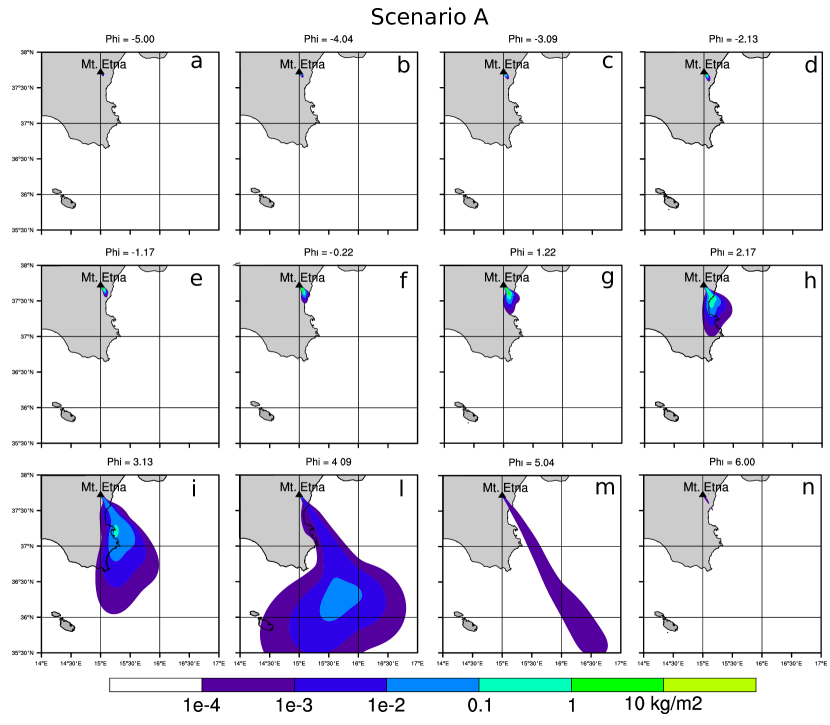
Figure A1: Computed ground loading contours [kg/m² ] for Scenario_A at the end of the simulation for different classes: A) $\phi=-5$ … E) $\phi=6$. Isomass contours are log-spaced from 10^-5 to $10$ [kg/m² ]. In all plots the black triangle indicates the position of the eruptive vent.

Fig. A1 shows a detailed deposit map for Scenario_A, where deposit (DM_i) is plotted for different particle classes: A) $\phi=-5$ … E) $\phi=6$. Isomass contours are log-spaced from 10^-5 to $10$ [kg/m² ]. Although smaller particles have a larger diffusion coefficient they are carried farther by the wind due to the low settling velocity. Therefore most of the finer particles ($\phi$ >4) are leaving the domain and only a few percent of the emitted mass (EM_i) is deposited on the ground over the considered domain. Finest simulated class ($\phi=6$), as shown in Fig A1n, is almost absent in the computed deposit. Moreover, we can notice that different classes present different main axis directions on the deposit. This segregation process is mostly due to a shear on the wind direction with the altitude. Smaller particles are more influenced by higher wind directions and consequently also their deposit trace. This suggests to be careful when inferring the main dispersal axis and consequently when choosing sampling locations. Wind measurements and reliable weather data are fundamental if we want to proper characterize the footprint left on the ground by an eruption.

In order to generalize the results presented in the main paper, we investigate here results dependency on the emitted grain size distribution (GSD). Fig. A2 shows the results of 110 runs where emitted GSD is chosen using 24 classes with a log-normal distribution described by different values of $\sigma$ and $\mu$. Each dot represents a different run and the color map is obtained interpolating the values of DM_i/EM_i from the dots location. Results are shown for three different classes $\phi=2$ (A), $\phi=4$ (B) and $\phi=6$ (C). For each of these classes the variability of DM_i/EM_i is really small ($3-4\%$ respect to the mean value), and for $\phi>4$ this ratio is even smaller. Therefore the percentage of deposited mass with respect to the emitted one is almost independent from the emitted GSD, allowing to generalize the results obtained for Scenario_A also to GSDs different from the original one presented in the manuscript.

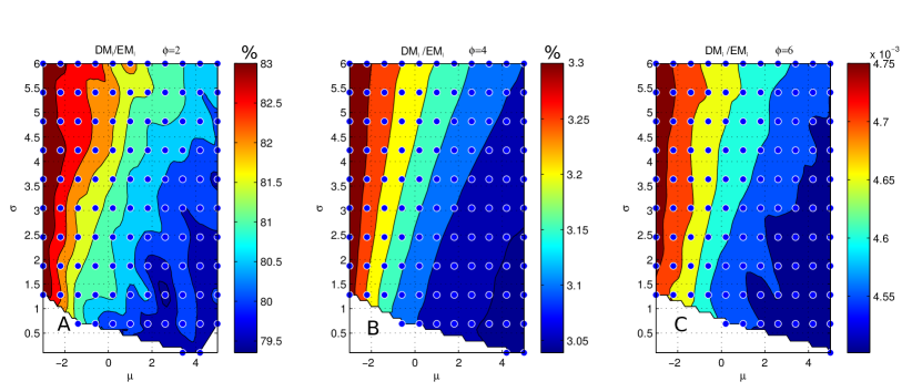
Figure A2: Deposited mass (DM_i) for different class sizes $\phi=2$ (A) $\phi=4$ (B) $\phi=6$ (C) expressed as a percentage of the (EM_i ). A blue dot represents a run made using as emitted GSD a log normal distribution with assigned parameters $\mu$ and $\sigma$. Colored surface is obtained interpolating the results over 110 simulations.

In addition to the analysis on the effect of the initial particles distribution, here we want to investigate the role of particle shape factor $\psi$ and density $\rho$ on the transport and deposition process. Several experimental studies have highlighted how an irregular shape of falling particles could affect their velocity toward the ground [15, 16, 17, 11, 9]. As introduced in [11] the sphericity parameter $\psi$ is defined as the ratio between the projected area $A_{p}$ and the square of the projected perimeter $P_{p}$:

$$\psi=\frac{4\pi A_{p}}{P_{p}^{2}}.$$

In Fig A3 deposited mass DM_i for different class sizes ($\phi=2$ (A), $\phi=4$ (B), $\phi=6$ (C)) is expressed as a percentage of the emitted mass EM_i. Each blue dot represents a run made using as emitted GSD a uniform distribution but with different factor shape $\psi\in[0.5,1]$ and density $\rho\in$ [1500, 2000] kg/m³. In Fig A3F is presented a schematic example of different particles with different sphericity values $\psi$. For spherical particles $\psi=1$. Colored contour plot is obtained interpolating the results over 121 simulations. In Fig. A3D and A3E) are plotted respectively as input response surfaces the emitted mass $EM_{tot}$ and averaged column height. We can notice that for a fixed $\phi$ class the ratio DM_i/EM_i increases with increasing density and sphericity. In fact more irregular and lighter particles are transported farther. Besides, relative changes in the DM_i/EM_i increases with the decreasing size: 0.3% for $\phi=2$, 7% $\phi=4$ and 8% for $\phi=6$. As expected EM_i (Fig A3D) increases with particles density and is not influenced by the sphericity, whereas denser particles produce lower column heights (see Fig A3E). Finally, less spherical are the particles, less rapid is their vertical displacement allowing a longer staying in the atmosphere.

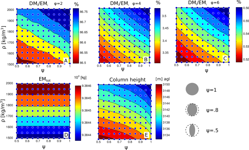
Figure A3: Deposited mass (DM_i) for different class sizes $\phi=2$ (A) $\phi=4$ (B) $\phi=6$ (C) expressed as a percentage of the emitted (EM_i ). A blue dot represents a run made using as emitted GSD a uniform distribution where particles have different factor shape $\psi\in[0.5,1]$ and density $\rho\in$ [1500, 2000] kg/m³. Colored surface is obtained interpolating the results over 121 simulations. D) Emitted mass and E) averaged column height. F) Schematic example of different particles with different sphericity $\psi$.

A.2 Uncertainty analysis

In order to quantify the interval of confidence of the fitting parameters and consequently of the estimated volume, different techniques have been recently introduced [8, 2, 3]. Model misspecification on fitting process may cause large bias thus leading to incorrect inference. In this section we want to understand how the uncertainty in eruption volume estimation is depending on the fitting model (for example the difference between applying the Weibull model vs the exponential model) and on fitting errors. First of all, we want to compare the intervals of confidence for the volume estimation obtained applying the different techniques presented in the manuscript. On [8] the estimation is based on a least-squares method. Relative squared error is used to measures how well a fitting function $f$ fits the data $y$. Errors are assumed normally distributed.

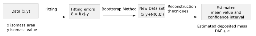
Figure A4: Schematic representation of the bootstrap method.

Here in a similar way of [3] we used a bootstrap Monte-Carlo method [10] as presented in Fig A4. In order to create a large dataset, the first step is to randomly perturb the calculated isomass area. If errors in the isomass squared area calculation ($y$ points) are available, then the random variation in each point is determined from its given error. Otherwise, the random variation is determined from average standard deviation of $y$ points. A large number of random data sets are then produced and fitted, and the variance of fit results is used as the error for the fit parameters. Even if estimations of observational errors have been produced for mass loading measurement [1], it not trivial to predetermine the error distribution on corresponding isomass area, especially for sparse sampling points dataset.

Test		Pyle	Power Law	Weibull1	Weibull2	Weibull3
	Residual norm	0.12	0.41	1.08	0.5	0.5
1 A	Mean Volume	0.55	0.81	34.8	6.42	6.42
	Residual norm	0.14	0.32	21	0.26	1.65
2 A	Mean Volume	1.3	1.36	66.3	1.49	1.49

Table A2: Residual norm, Volume mean and Volume error estimate for all the volume reconstruction methods. Error estimation is calculated using a boot strap method. Values are expressed as a fraction of the emitted volume.

Bootstrap method has been applied to the volume reconstruction techniques from two selected tests (TestA_1, TestA_2) using 1000 "perturbed" $y$-data sets. Analysis results are presented in table A2. We can notice the following main facts:

• a small residual norm (i.e. a good fitting) does not guarantee a small interval of confidence.

• estimate error and consequently the estimate confidence interval are not representative of the real error committed.

Moreover, comparing the three different Weibull methods, we observe that results strongly depend on the choice of the residual function, and generally the volume mean is smaller than the volume errors. Unfortunately, it is difficult to find a non-subjective criterion for choosing the appropriate residual function. Even if we can find a satisfactory fitting of the mass loading vs squared area, this does not ensure a good volume estimation when errors are also associated with area values.

However the estimation is based on the assumption that the fitting model is valid, and does not account for error in the interpolation of the isomass contours from sparse data. Finally we have to stress that, to a lesser extent, the mass estimation methods proposed are also sensitive to the values and the number of isomasses.

A.3 Aggregation

As stated in several papers [6, 4, 13, 5], particle aggregation can significantly affect the dispersal process and the tephra depositional pattern. For this reason we extended our results considering a simple aggregation process. As proposed by [14] aggregation is supposed occurring within the margin of the column. To this aim, we adopt a model based on [7, 12], where $10-50\%$ of emitted mass for $\phi>2$ particles aggregates as $\phi=2$ ($250$ $\mu m$ ) particles. As a first approximation particle density is not modified and is equals to 2000 kg/m³. As stated by [5]), aggregates, due to the collision on the ground and during measurements are supposed to be found as completely break apart on the deposit.

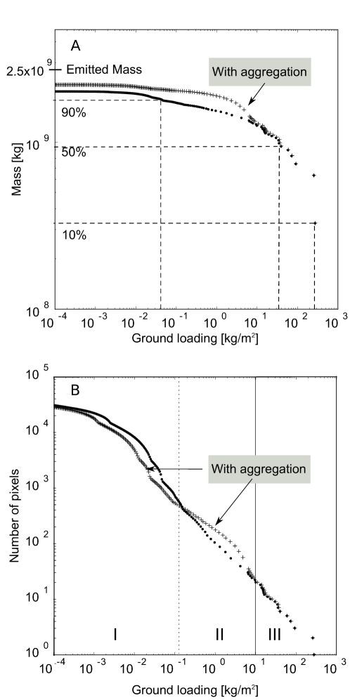
Figure A5: A) Cumulative mass versus mass loading. Dashed lines denote the $10\%$ , $50\%$ and $90\%$ of the total deposited mass and the corresponding ground loading. Black segment corresponds to the EM_tot equal to $2.5\cdot 10^{9}$ kg. B) Figures shows results without (dots) or with $50\%$ degree of aggregation (crosses). We can identify three intervals in ground loading values where the crosses (simulations with aggregation) are respectively below (interval I) (at distance), above (interval II) (intermediate) or coincident (interval III) (proximal).

In Fig.A5A cumulative mass is plotted as a function of ground loading. Total emitted mass (EM_tot), equal to 2.5 $\cdot$ 10⁹ kg, is reported on the left y-axis. This reveals how DM_tot corresponds to about 82$\%$ of EM_tot, even though the calculation has been obtained considering ground loading values down to 10^-4 kg/m² over an extended domain. In these figures, for the simulations without aggregation, we also plotted, with black dashed lines, the 10$\%$, 50$\%$ and 90$\%$ of the total deposited mass ( DM_tot) and the corresponding ground loading which is, respectively of 3.0$\cdot$10², 30 and 4$\cdot$10^-2 kg/m². Results are shown considering no aggregation (dots) or with $50\%$ degree of aggregation (crosses). When $50\%$ of aggregation is introduced in the model, a larger amount of mass is deposited within the domain, resulting in an increase of $10\%$ for Scenario_A. Fig. A5B shows cumulative pixels number calculated as a function of mass loading for simulation with and without aggregation. Three intervals can be identify in ground loading values, where the crosses (simulations with aggregation) are respectively below (interval I) (at distance), above (interval II) (intermediate) or coincident (interval III) (proximal) with the dots (simulations without aggregation). These intervals depend on the way aggregation is modelled (in this study on the percentages assumed to aggregate) and, above all, on the dimension of the aggregates and their fall velocities. Most of the particles involved in the aggregation process do not fall in proximal areas. Consequently, close to the vent, where the cumulative ground loading is larger than 10 kg/m² aggregation has a negligible effect (interval III). Below these values aggregation reveals its main effects. In particular, in the range $[10^{-1},10]$ kg/m² (interval II) a large portion of particles falls over a smaller area with higher loadings. At the same time, the area corresponding to low loading values, here smaller than $10^{-1}$ kg/m² (interval I), is reduced.

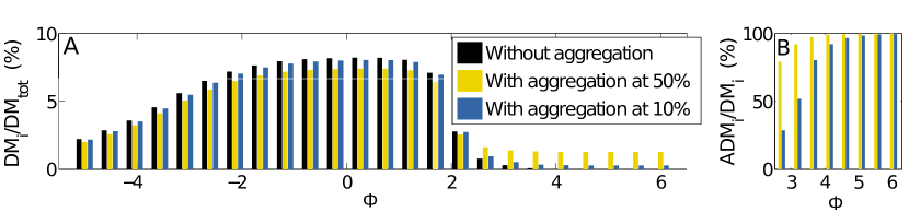
Figure A6: A) i-th deposited mass ( DM_i ) expressed as percentage of total deposited mass ( DM_tot ). Different colors correspond to different degrees of aggregation: no aggregation (black), 50% (yellow), 10% (blue). B) i-th mass deposited as aggregate (ADM_i) expressed as percentage of i-th deposited mass (DM_i ) . Results have been obtained: i) excluding an area within a distance of about 2 km from the vent ii) considering a ground loading $>0.1$ kg/m² and iii) limiting the calculations only to the deposit fallen on the land.

This is also shown in Fig. A6A and A6C, where the TGSD is plotted for different aggregation percentages ($0\%$ - black, $10\%$ - blue and $50\%$ - yellow).

In Fig. A6B it is also plotted, for each aggregating i-class (finer than $\phi$ =3), the mass deposited as aggregate (ADM_i) expressed as percentage of the deposited one (DM_i). As expected the amount of deposited fine particles increases proportionally with aggregation. Nevertheless, even when $10\%$ and $50\%$ of aggregation is considered, for $\phi=5$ and $\phi=6$ classes deposit only as aggregates ( ADM_i/DM_i=100% ) in the considered domain,

This plot reveals how using these ratio as indicative of the degree of aggregation of sampled particles can be misleading. Indeed, the observation of a particular class in the deposit only as aggregate could be erroneously interpreted as evidence that $100\%$ of the emitted mass for the i-class aggregated during the transport.

References

- [1] B Bernard “Homemade ashmeter: a low-cost, high-efficiency solution to improve tephra field-data collection for contemporary explosive eruptions” In Journal of Applied Volcanology 2:1, 2013 DOI: 10.1186/2191-5040-2-1
- [2] S Biass and C Bonadonna “A quantitative uncertainty assessment of eruptive parameters derived from tephra deposits: the example of two large eruptions of Cotopaxi volcano and Ecuador” In Bull Volcanol 73, 2011, pp. 73–90
- [3] S Biass, G Bagheri, WH Aeberhard and C Bonadonna “TError: towards a better quantification of the uncertainty propagated during the characterization of tephra deposits” In Statistics in Volcanology 1, 2013, pp. 1–27 DOI: 10.5038/2163-338X.1.2
- [4] C Bonadonna et al. “Determination of the largest clasts of tephra deposits for the characterization of explosive volcanic eruptions: report of the IAVCEI Commission on Tephra Hazard Modelling”, 2011 URL: https://vhub.org/resources/870
- [5] RJ Brown, C Bonadonna and AJ Durant “A review of volcanic ash aggregation” In Physics and Chemistry of the Earth 45-46, 2012, pp. 65–78
- [6] SN Carey and H Sigurdsson “Influence of particle aggregation on deposition of distal tephra from the May 18 and 1980 and eruption of Mount St. Helens Volcano” In J Geophys Res 87, 1982, pp. 7061–7072
- [7] W Cornell, S Carey and H Sigurdsson “Computer simulation of transport and deposition of the Campanian Y-5 ash” In J Volcanol Geotherm Res 17, 1983, pp. 89–109
- [8] ML Daggitt, TA Mather, DM Pyle and S Page “AshCalc-a new tool for the comparison of the exponential and power-law and Weibull models of tephra deposition” In Journal of Applied Volcanology 3, 2014
- [9] P Dellino et al. “The analysis of the influence of pumice shape on its terminal velocity” In Geophys. Res. Lett. 32, 2005 DOI: 10.1029/2005GL023954
- [10] B Efron and R Tibshirani “An Introduction to the Bootstrap”, 1993
- [11] CM Riley, WI Rose and GJS Bluth “Quantitative shape measurements of distal volcanic ash” In J. Geophys. Res 108, B10, 2003, pp. 2504 DOI: 10.1029/2001JB000818
- [12] R Sulpizio et al. “Hazard assessment of far-range volcanic ash dispersal from a violent Strombolian eruption at Somma-Vesuvius volcano and Naples and Italy: implications on civil aviation” In Bull Volcanol 74 9, 2012, pp. 2205–2218
- [13] J Taddeucci et al. “Aggregation-dominated ash settling from the Eyjafjallajökull volcanic cloud illuminated by field and laboratory high-speed imaging” In Geology 39, 2011, pp. 891–894
- [14] C Textor et al. “Volcanic particle aggregation in explosive eruption columns. Part I: Parameterization of the microphysics of hydrometeors and ash” In J Volcanol Geotherm Res 150, 2006, pp. 359–377
- [15] GPL Walker “Grain-size characteristics of pyroclastic deposits” In J. Geol 79, 1971, pp. 696
- [16] L Wilson “Explosive volcanic eruptions - II The atmospheric trajectories of pyroclast” In Geophys. J. R. astr. Soc 30, 1972, pp. 381–392
- [17] L Wilson and TC Huang “The influence of shape on the atmospheric settling velocity of volcanic ash particles” In Earth Planet Sci Lett 44, 1979, pp. 311–324