A higher-order gradient flow scheme for a singular one-dimensional diffusion equation

Abstract.

A nonlinear diffusion equation, interpreted as a Wasserstein gradient flow, is numerically solved in one space dimension using a higher-order minimizing movement scheme based on the BDF (backward differentiation formula) discretization. In each time step, the approximation is obtained as the solution of a constrained quadratic minimization problem on a finite-dimensional space consisting of piecewise quadratic basis functions. The numerical scheme conserves the mass and dissipates the $G$-norm of the two-step BDF time approximation. Numerically, also the discrete entropy and variance are decaying. The decay turns out to be exponential in all cases. The corresponding decay rates are computed numerically for various grid numbers.

1. Introduction

The aim of this paper is to propose and study a fully discrete higher-order variant of the minimizing movement scheme in one space dimension for the nonlinear diffusion equation

(1) $$\partial_{t}u=\alpha^{-1}\Delta(u^{\alpha})\quad\mbox{in }{\mathbb{T}}^{d},\ t>0,\quad u(0)=u^{0},$$

with negative exponent $\alpha<0$, where ${\mathbb{T}}^{d}$ is the $d$-dimensional torus. Equation (1) can be written as the gradient flow of the entropy $S[u]=(\alpha(\alpha-1))^{-1}\int_{{\mathbb{T}}^{d}}u^{\alpha}dx$ with respect to the Wasserstein distance. The gradient flow formulation gives rise to a natural semi-discretization in time of the evolution by means of the minimizing movement scheme, leading to a minimization problem for the sum of kinetic and potential energies.

Minimizing movement schemes for evolution equations with an underlying gradient flow structure were first suggested by De Giorgi [12] in an abstract framework. Jordan, Kinderlehrer, and Otto [17] have shown that the solution to the linear Fokker-Planck equation can be obtained by minimizing the logarithmic entropy in the Wasserstein space. Since then, many nonlinear evolution equations have been shown to constitute Wasserstein gradient flows, for instance the porous-medium equation [23], the Keller-Segel model [4], equations for interacting gases [10], and a nonlinear fourth-order equation for quantum fluids [14].

The minimizing movement scheme can be interpreted as an implicit Euler semi-discretization with respect to the Wasserstein gradient flow structure. While for some time this has been mainly used as an analytical tool, more recently numerical approximations of evolution equations using this scheme have been proposed. In one space dimension, the optimal transport metric becomes flat when re-parametrized by means of inverse cumulative functions, which simplifies the numerical solution; see e.g. [1, 4, 20, 22]. For multi-dimensional situations, one approach is based on the Eulerian representation of the discrete solution on a fixed grid. The resulting problem can be solved by using interior point methods [8], finite elements [7], or finite volumes [9]. Another approach employs the Lagrangian representation, which is well adapted to optimal transport. Examples are explicit marching schemes [15], moving meshes [6], linear finite elements for a fourth-order equation [13], reformulations in terms of evolving diffeomorphisms [11], and entropic smoothing using the Kullback-Leibler divergence [24]. The connection between Lagrangian schemes and the gradient flow structure was investigated in [19]. In this paper, we will use the Lagrangian viewpoint.

The minimizing movement scheme of De Giorgi is of first order in time only since it is based on the implicit Euler method. Concerning higher-order schemes, we are only aware of the paper [31]. There, second-order gradient flow schemes were suggested for the Euler equations, with finite differences in space and the two-step BDF (Backward Differentiation Formula) method or diagonally implicit Runge-Kutta (DIRK) schemes in time.

In this paper, we propose a fully discrete second-order minimizing movement scheme using quadratic finite elements in space and the two-step BDF method in time. We consider periodic point-symmetric solutions. The finite-dimensional minimization problem, constrained by the mass conservation, is solved by the method of Lagrange multipliers which leads to a sequential quadratic programming problem.

By construction, our numerical scheme is of second order both in time and space, it conserves the mass and dissipates the $G$-norm of the approximation $\mathbf{g}^{k}$ of the quadratic ansatz functions at time step $k$,

(2) $$\|(\mathbf{g}^{k+1},\mathbf{g}^{k})\|_{G}^{2}=\frac{5}{2}(\mathbf{g}^{k+1})^{\top}M_{w}\mathbf{g}^{k+1}-2(\mathbf{g}^{k+1})^{\top}M_{w}\mathbf{g}^{k}+\frac{1}{2}(\mathbf{g}^{k})^{\top}M_{w}\mathbf{g}^{k},$$

where the matrix $M_{w}$ is defined in the approximation of the Wasserstein metric on the space of the quadratic ansatz functions. We refer to Section 3 for details. It turns out that numerically, the relative $G$-norm decays exponentially fast to zero. Although we cannot expect for the multistep scheme that the discrete entropy decays exponentially fast, this holds true for the numerical experiments performed in this paper. Furthermore, also the discrete variance of the original variable $u$ and the Lagrangian variable decay exponentially fast.

The numerical tests also indicate that the decay rate of the entropy is increasing in the number of grid points, i.e., the discrete decay rates are smaller than the (expected) value for the continuous equation. This result is in accordance with the findings of [21] for a finite-volume approximation of a one-dimensional linear Fokker-Planck equation.

Let us briefly review the literature for the diffusion equation (1) with $\alpha<0$. Equation (1) with $\alpha=-1$ appears in the modeling of heat conduction in solid Helium, where the solution $u$ corresponds to the inverse temperature [26]. When this equation is considered in the whole space or in a bounded domain with homogeneous Dirichlet boundary conditions, it is sometimes called the super-fast diffusion equation [28, Chap. 9]. The critical exponent of this equation in one space dimension is $\alpha=-1$. For $\alpha>-1$ and $u^{0}\in L^{1}(\mathbb{R})$, we have a smoothing property, namely $u(t)\in L^{\infty}(\mathbb{R})$ for any $t>0$ [28, Section 9.1]. For $\alpha\leq-1$, no solutions exist with data in $L^{1}(\mathbb{R})$. The non-existence range in dimensions $d\geq 2$ contains even all negative exponents, $\alpha<0$ [27]. However, if $d=1$ and $\alpha\leq-1$, there is a weak smoothing effect. Indeed, given $u^{0}\in L_{\rm loc}^{p}(\mathbb{R})$ for $p=(1-\alpha)/2$, the solution $u$ exists and is locally bounded in $\mathbb{R}\times(0,\infty)$. Furthermore, if $u^{0}\in L^{p}(\mathbb{R})$ then there is instantaneous extinction, i.e. $u(t)=0$ in $\mathbb{R}$ for all $t>0$ [28, Theorem 9.3].

Clearly, such results cannot be expected when the super-fast diffusion equation is considered on the torus. We expect that global-in-time weak solutions exist, which converge to the constant steady state as $t\to\infty$. Since we could not find any results on the existence and large-time asymptotics in the literature in that situation and since the use of negative exponents is less standard, we provide a (short) proof for completeness in the appendix; see Section 2.1 for details.

The paper is organized as follows. The global existence result and the exponential decay of the solutions to the constant steady state as well as some basic properties of the Wasserstein distance for periodic functions are stated in Section 2. Section 3 is devoted to the description of the numerical scheme, and some numerical experiments are presented in Section 4. We conclude in Section 5. The appendix contains the proofs of the existence and large-time asymptotics theorems and the calculations of the coefficients of the matrix $M_{w}$ and the Hessian of the discrete entropy.

2. Prerequisites

2.1. Existence of solutions and large-time asymptotics

Equation (1) on the torus ${\mathbb{T}}^{d}$ does not possess the non-existence or instantaneous extinction properties of the super-fast diffusion equation in the whole space since mass cannot get lost. In fact, we expect that for any $\alpha<0$, there exists a global weak solution. If the initial datum $u^{0}$ is nonnegative only, (1) is still a singular diffusion equation. However, because of the fast diffusion, the solution becomes positive for all positive times and, by parabolic regularity theory, also smooth.

Theorem 1 (Existence of weak solutions).

Let $\alpha<0$ and let $u^{0}\in L^{\infty}({\mathbb{T}}^{d})$ satisfy $u^{0}\geq 0$. If $\alpha=-1$, we assume additionally that $\int_{{\mathbb{T}}^{d}}\log u^{0}dx>-\infty$. Then there exists a unique weak solution to (1) satisfying $u^{\alpha}\in L^{2}(0,T;H^{1}({\mathbb{T}}^{d}))$, $\partial_{t}u\in L^{2}(0,T;H^{1}({\mathbb{T}}^{d})^{\prime})$ for all $T>0$, and $0\leq u(x,t)\leq\sup_{{\mathbb{T}}^{d}}u^{0}$ for $x\in{\mathbb{T}}^{d}$, $t\geq 0$.

The proof of this theorem is based on a standard regularization procedure but we need to distinguish carefully the cases $-1<\alpha<0$, $\alpha=-1$, and $\alpha<-1$. We present the (short) proof for completeness in Appendix A. For $t\to\infty$, the (smooth) solution converges to the constant steady state. Since this constant is positive, diffusion slows down when time increases. Therefore, we cannot expect instantaneous extinction phenomena. Still, we are able to prove that the convergence is exponentially fast with respect to the $L^{1}$-norm. We introduce the entropy

$$H_{\beta}[u]=\int_{{\mathbb{T}}^{d}}u^{\beta}\,dx-\bigg{(}\int_{{\mathbb{T}}^{d}}u\,dx\bigg{)}^{\beta},\quad\beta>1.$$

The steady state of (1) is given by $u_{\infty}=\int_{{\mathbb{T}}^{d}}u^{0}\,dx$ if $\mbox{vol}({\mathbb{T}}^{d})=1$.

Theorem 2 (Exponential decay).

Let $u$ be a smooth positive solution to (1) and let $\text{\rm vol}({\mathbb{T}}^{d})=1$. Then

$$\|u(t)-u_{\infty}\|_{L^{1}({\mathbb{T}}^{d})}\leq C_{\beta}H_{\beta}[u^{0}]^{1/\beta}\|u^{0}\|_{L^{1}({\mathbb{T}}^{d})}^{1/2}e^{-\lambda t},$$

where $C_{\beta}>0$ and for $\alpha<0$, $1<\beta\leq 2$,

$$\lambda=\frac{2(\beta-1)}{\beta C_{B}}(\sup_{{\mathbb{T}}^{d}}u^{0})^{\alpha-1},$$

and $C_{B}>0$ is the constant in the Beckner inequality (19); for $-1\leq\alpha<0$, $\beta=2(1-\alpha)$,

$$\lambda=\frac{2(1-2\alpha)}{(1-\alpha)\|u^{0}\|_{L^{1}({\mathbb{T}}^{d})}^{1-\alpha}}.$$

In the first result, the decay rate $\lambda$ depends on $\sup_{{\mathbb{T}}^{d}}u^{0}$, which seems to be not optimal. The decay rate in the second result depends on the $L^{1}$-norm of $u^{0}$ only but we need a particular value of $\beta$. The proof is based on the entropy method; see Appendix A. Stronger decay results have been derived for the fast-diffusion equation in the whole space or in bounded domains; see, e.g., [5, 28]. However, our proof is very elementary and just an illustration for the qualitative behavior of the solutions to (1).

2.2. The Wasserstein distance for periodic functions

We recall some basic facts about mass transportation and Wasserstein distances following [13]. For more details, we refer to [2, 30]. Let $X$ be a Riemannian manifold with distance $d:X\times X\to\mathbb{R}_{+}:=[0,\infty)$ and let $P_{M}(X)$ be the convex set of measures with fixed mass $M>0$ on $X$. The $L^{2}$-Wasserstein distance of two measures $\mu_{1}$, $\mu_{2}\in P_{M}(X)$ is defined by

(3) $$W[\mu_{1},\mu_{2}]^{2}=\inf_{\pi\in\Pi(\mu_{1},\mu_{2})}\int_{X\times X}d(x,y)^{2}\,d\pi(x,y),$$

where $\Pi(\mu_{1},\mu_{2})$ is the set of transport plans connecting $\mu_{1}$ with $\mu_{2}$, i.e. the set of all measures on $X\times X$ with respective marginals $\mu_{1}$ and $\mu_{2}$,

$$\pi(A\times X)=\mu_{1}(A),\quad\pi(X\times B)=\mu_{2}(B)$$

for all measurable sets $A$, $B\subset X$. If the measures $\mu_{1}$ and $\mu_{2}$ possess densities $u_{1}$ and $u_{2}$, respectively, with respect to a fixed measure on $X$, then we write, slightly abusing the notation, $W[u_{1},u_{2}]$ instead of $W[\mu_{1},\mu_{2}]$.

In one space dimension, there exists an explicit formula to compute $W$. Let $X=(a,b)\subset\mathbb{R}$ be a (possibly infinite) interval, and let $\mu_{1}$, $\mu_{2}\in P_{M}(X)$ be two measures. We define their distribution functions

$$U_{i}:(a,b)\to[0,M],\quad U_{i}(x)=\mu_{i}((a,x]),\quad i=1,2.$$

As these functions are right-continuous and monotonically increasing, they possess right-continuous increasing pseudo-inverse functions $G_{i}:[0,M]\to[a,b]$, given by

$$G_{i}(\omega)=\inf\{x\in(a,b):U_{i}(x)>\omega\},\quad i=1,2.$$

Then [29],

(4) $$W[u_{1},u_{2}]^{2}=\int_{0}^{M}(G_{1}(\omega)-G_{2}(\omega))^{2}d\omega.$$

This formula does not extend to $X={\mathbb{T}}\simeq(0,1)$ because of the topology induced by the periodic boundary conditions, $d(x,y)=\min\{|x-y|,1-|x-y|\}$. The reason is that mass can be transported either clock- or counter-clockwise (see [13] for details). However, if the densities $u_{1}$ and $u_{2}$ are point-symmetric, (4) still holds. More precisely, let $u_{i}(x)=u_{i}(1-x)$ for $x\in(0,1)$ and $i=1,2$. Then (4) holds, where $G_{i}:[0,M]\to[0,1]$ is the inverse function of $U_{i}(x)=\int_{0}^{x}u_{i}(y)dy$ [13, Lemma 2.2].

3. Time discretization and Lagrangian coordinates

3.1. The semi-discrete BDF scheme

We introduce the second-order minimizing movement scheme. First, we explain the underlying idea for the finite-dimensional gradient flow

(5) $$\dot{x}=-\nabla\phi(x),\quad t>0,\quad x(0)=x_{0},$$

where $\phi:\mathbb{R}^{d}\to\mathbb{R}$ is a smooth potential. This equation can be approximated by the following minimization problem:

$$x^{n+1}=\operatorname*{argmin}_{x\in\mathbb{R}^{d}}\Phi(x),\quad\Phi(x)=\frac{1}{2\tau}\|x-x^{n}\|^{2}+\phi(x),$$

where $\tau>0$ is the time step size and $x^{n}$ is an approximation of $x(n\tau)$. The minimizer $x^{n+1}$ is a critical point and thus,

$$0=\nabla\Phi(x^{n+1})=\frac{1}{\tau}(x^{n+1}-x^{n})+\nabla\phi(x^{n+1}),$$

which corresponds to the implicit Euler scheme.

Instead of the Euler scheme, we wish to discretize (1) by a multistep method. As an example, consider the two-step BDF (or BDF-2) method,

$$\frac{1}{\tau}\left(\frac{3}{2}x^{n+2}-2x^{n+1}+\frac{1}{2}x^{n}\right)=-\nabla\phi(x^{n+2}),$$

where $x^{n}$ and $x^{n+1}$ are given. Writing this scheme as

$$\frac{1}{2}(x^{n}-x^{n+2})-2(x^{n+1}-x^{n+2})=-\tau\nabla\phi(x^{n+1}),$$

we see that $x^{n+2}$ is a critical point of the functional

$$\Phi(x)=-\frac{1}{4\tau}\|x^{n}-x\|^{2}+\frac{1}{\tau}\|x^{n+1}-x\|^{2}+\phi(x).$$

More generally, the BDF-$k$ approximation of (5),

$$\sum_{i=0}^{k}a_{i}x^{n+i}=-\tau\nabla\phi(x^{n+k}),$$

for given $x^{n},\ldots,x^{n+k-1}$ can be formulated as

$$-\tau\nabla\phi(x^{n+k})=\sum_{i=0}^{k-1}a_{i}x^{n+i}+a_{k}x^{n+k}=\sum_{i=0}^{k-1}a_{i}(x^{n+i}-x^{n+k}),$$

since $\sum_{i=0}^{k}a_{i}=0$, or as the minimization problem

(6) $$x^{n+k}=\operatorname*{argmin}_{x\in\mathbb{R}^{d}}\Phi(x),\quad\Phi(x)=-\frac{1}{2\tau}\sum_{i=0}^{k-1}a_{i}\|x^{n+i}-x\|^{2}+\phi(x),$$

In a similar way, we may formulate general multistep methods. We recall that BDF-$k$ schemes are consistent if $\sum_{i=0}^{k}a_{i}=0$, $\sum_{i=1}^{k}ia_{i}=1$ and zero-stable if and only if $k\leq 5$ [25, Section 11.5].

The same idea as above is applicable to gradient flows in the $L^{2}$-Wasserstein distance. For this, we replace the $L^{2}$ norm by the Wasserstein distance. For equation (1), scheme (6) turns into

(7) $$u^{n+k}=\operatorname*{argmin}_{u\in P_{M}({\mathbb{T}})}\Phi(u),\quad\Phi(u)=-\frac{1}{2\tau}\sum_{i=0}^{k-1}a_{i}W[u^{n+i},u]^{2}+S[u],$$

where $S[u]=(\alpha(\alpha-1))^{-1}\int_{\mathbb{T}}u^{\alpha}\,dx$. Scheme (7) can be interpreted as a BDF-$k$ minimizing movement scheme.

3.2. Lagrangian coordinates

Before introducing the spatial discretization, we rewrite the scheme (7) in a more explicit manner, using the inverse distribution functions $G$ and $G^{*}$ of $u$ and $u^{*}$, respectively, which were introduced in Section 2.2. The numerical procedure is similar to that in [13] but our higher-order scheme introduces some changes. We call $\omega=U(x)\in[0,M]$ the Lagrangian coordinate, which is conjugate to the Eulerian coordinate $x\in{\mathbb{T}}$, and we refer to the inverse distribution function $G$ as the associated Lagrangian map. For a consistent change of variables, we need to express the entropy $S[u]$ in terms of the Lagrangian coordinates. With the formula for the differential of an inverse function,

$$u(x)=\partial_{x}U(x)=\frac{1}{\partial_{\omega}G(\omega)},$$

and the change of unknowns $x=G(\omega)$ under the integral in $S[u]$, we obtain

$$S[u]=\frac{1}{\alpha(\alpha-1)}\int_{\mathbb{T}}\frac{u(x)\,dx}{u(x)^{1-\alpha}}=\frac{1}{\alpha(\alpha-1)}\int_{\mathbb{T}}g(\omega)^{1-\alpha}\,d\omega,$$

where $g(\omega)=\partial_{\omega}G(\omega)$. Note that the exponent in the integrand is positive since $\alpha<0$. In terms of $g$, the expression for the Wasserstein distance in (4) becomes (see [13, Section 2.3])

$$W[u,u^{*}]^{2} =\int_{0}^{M}(G(\omega)-G^{*}(\omega))^{2}\,d\omega=\int_{0}^{M}\bigg{(}\int_{0}^{\omega}(g(\eta)-g^{*}(\eta))d\eta\bigg{)}^{2}\,d\omega$$

$$=\int_{0}^{M}\int_{0}^{M}(M-\max\{\eta,\eta^{\prime}\})(g(\eta)-g^{*}(\eta))(g(\eta^{\prime})-g^{*}(\eta^{\prime}))\,d\eta\,d\eta^{\prime}.$$

This expression is simply a quadratic form in $g-g^{*}$ and thus easy to implement in the numerical scheme. We summarize our results which slightly generalize Lemma 2.3 in [13].

Lemma 3.

Let the initial datum $u^{0}:{\mathbb{T}}\to\mathbb{R}$ be point-symmetric. Then the solution $u^{n+k}$ to the BDF-$k$ scheme (7) is in one-to-one correspondence to the solution $g^{n+k}$ obtained from the inductive scheme

(8) $$g^{n+k}=\operatorname*{argmin}_{g}\Psi(g),$$

with initial condition $g^{0}=1/u\circ G$ and given $g^{1},\ldots,g^{n+k-1}$ obtained from a lower-order scheme. The argmin has to be taken over all measurable functions $g:[0,M]\to(0,\infty)$ satisfying the mass constraint $\int_{0}^{M}g(\omega)\,d\omega=1$, and the function $\Psi$ is given by

(9) $$\Psi(g) =-\frac{1}{2\tau}\int_{0}^{M}\int_{0}^{M}(M-\max\{\eta,\eta^{\prime}\})\sum_{i=0}^{k-1}a_{i}(g(\eta)-g^{n+i}(\eta))(g(\eta^{\prime})-g^{n+i}(\eta^{\prime}))\,d\eta\,d\eta^{\prime}$$

$$\phantom{xx}{}+\frac{1}{\alpha(1-\alpha)}\int_{0}^{M}g(\omega)^{1-\alpha}\,d\omega.$$

Moreover, $\Phi(u)=\Psi(g)$ and the functions $u^{n}$ and $g^{n}$ are related by

(10) $$u^{n}(x_{\omega})=\frac{1}{g^{n}(\omega)},\quad x_{\omega}=\int_{0}^{\omega}g^{n}(\eta)\,d\eta.$$

In Lagrangian coordinates, the problem has become a minimization problem in $\Psi(g)$ which is the sum of a quadratic form and a convex functional, hence it is convex. In the special case $\alpha=-1$, the second integral in (9) is quadratic too which simplifies the numerical discretization. Therefore, we will consider mainly numerical examples with $\alpha=-1$ in Section 4.

3.3. Spatial discretization

We approximate the infinite-dimensional variational problem (8) by a finite-dimensional one. Minimization in (8) is performed over the finite-dimensional space of quadratic ansatz functions. This generalizes the approach in [13], where only linear ansatz functions were used. We define the ansatz space as follows.

Let $N\in{\mathbb{N}}$ and a mesh $\{x_{0},\ldots,x_{N}\}$ on $[0,1]$ be given with $x_{0}=0$ and $x_{N}=1$. Using (10), we construct the mesh $\Omega_{N}=\{\omega_{0},\omega_{1}\ldots,\omega_{N}\}$ of $[0,M]$. Then $\omega_{0}=0$, $\omega_{N}=M$, $\omega_{i}<\omega_{i+1}$, and $\omega_{N-i}=M-\omega_{i}$ (point-symmmetry), where $i=1,\ldots,N-1$. Since we wish to introduce quadratic ansatz functions, we add the grid points $\omega_{j+1/2}=(\omega_{j+1}+\omega_{j})/2$ for $j=0,\ldots,N-1$.

The basis functions $\phi_{j}:{\mathbb{T}}\to\mathbb{R}$ are defined by

$$\phi_{j}(\omega) =\left\{\begin{array}[]{ll}\frac{\omega-\omega_{j-1}}{\omega_{j}-\omega_{j-1}}&\quad\mbox{for }\omega\in[\omega_{j-1},\omega_{j}],\\ \frac{\omega_{j+1}-\omega}{\omega_{j+1}-\omega_{j}}&\quad\mbox{for }\omega\in[\omega_{j},\omega_{j+1}],\\ 0&\quad\mbox{otherwise},\end{array}\right.\qquad j=1,\ldots,N-1,$$

$$\phi_{N}(\omega) =\left\{\begin{array}[]{ll}\frac{\omega_{1}-\omega}{\omega_{1}}&\quad\mbox{for }\omega\in[0,\omega_{1}],\\ \frac{\omega-\omega_{N-1}}{M-\omega_{N-1}}&\quad\mbox{for }\omega\in[\omega_{N-1},M],\\ 0&\quad\mbox{otherwise}.\end{array}\right.$$

This set of piecewise linear functions is supplemented by the following piecewise quadratic basis functions:

$$\phi_{N+j}(\omega)=\left\{\begin{array}[]{ll}1-\big{(}\frac{2\omega-(\omega_{j-1}+\omega_{j})}{\omega_{j}-\omega_{j-1}}\big{)}^{2}&\quad\mbox{for }\omega\in[\omega_{j-1},\omega_{j}],\\ 0&\quad\mbox{otherwise},\end{array}\right.\qquad j=1,\ldots,N.$$

The ansatz space is the set of all positive, piecewise quadratic functions $g:[0,M]\to\mathbb{R}_{+}$ of the form

(11) $$g(\omega)=\sum_{j=1}^{2N}g_{j}\phi_{j}(\omega).$$

We call $\mathbf{g}:=(g_{1},\ldots,g_{2N})\in[0,\infty)^{2N}$ the associated weight vector. By definition of $\phi_{j}$, we have $g(\omega_{j})=g_{j}$ for $j=1,\ldots,N$. Moreover, as $g$ is point-symmetric, $g_{0}=g_{N}$.

Now, for given mass $M>0$ and grid $\Omega_{N}\subset[0,M]$, we define the set ${\mathbb{G}}^{N}_{M}\subset\mathbb{R}_{+}^{2N}$ as the set of weight vectors $\mathbf{g}$ for which the associated interpolation $g$ from (11) satisfies the mass constraint,

(12) $$1=\int_{0}^{M}g(\omega)\,d\omega=\sum_{j=1}^{N}\left(\frac{g_{j-1}+g_{j}}{2}+\frac{2}{3}g_{N+j}\right)(\omega_{j}-\omega_{j-1}).$$

The Wasserstein metric for functions approximated in this way becomes

$$W[u,u^{*}]^{2} =\int_{0}^{M}\int_{0}^{M}(M-\max\{\eta,\eta^{\prime}\})\sum_{i=1}^{2N}(g_{i}-g_{i}^{*})\phi_{i}(\eta)\sum_{j=1}^{2N}(g_{j}-g_{j}^{*})\phi_{j}(\eta^{\prime})\,d\eta\,d\eta^{\prime}$$

$$=\sum_{i,j=1}^{N}(g_{i}-g_{i}^{*})(g_{j}-g_{j}^{*})a_{ij}+\sum_{i,j=1}^{N}(g_{N+i}-g_{N+i}^{*})(g_{j}-g_{j}^{*})b_{ij}$$

$$\phantom{xx}{}+\sum_{i,j=1}^{N}(g_{i}-g_{i}^{*})(g_{N+j}-g_{N+j}^{*})b_{ji}+\sum_{i,j=1}^{N}(g_{N+i}-g_{N+i}^{*})(g_{N+j}-g_{N+j}^{*})c_{ij},$$

where

$$a_{ij} =\int_{0}^{M}\int_{0}^{M}(M-\max\{\eta,\eta^{\prime}\})\phi_{i}(\eta)\phi_{j}(\eta^{\prime})\,d\eta\,d\eta^{\prime},$$

(13) $$b_{ij} =\int_{0}^{M}\int_{0}^{M}(M-\max\{\eta,\eta^{\prime}\})\phi_{N+i}(\eta)\phi_{j}(\eta^{\prime})\,d\eta\,d\eta^{\prime},$$

$$c_{ij} =\int_{0}^{M}\int_{0}^{M}(M-\max\{\eta,\eta^{\prime}\})\phi_{N+i}(\eta)\phi_{N+j}(\eta^{\prime})\,d\eta\,d\eta^{\prime}.$$

The coefficients $a_{ij}$, $b_{ij}$, and $c_{ij}$ can be computed explicitly. The explicit expressions are given in Appendix B.1. Setting $A=(a_{ij})$, $B=(b_{ij})$, $C=(c_{ij})$, and defining the matrix

(14) $$M_{w}=(M_{ij})=\begin{pmatrix}A&B^{\top}\\ B&C\end{pmatrix},$$

we can formulate the above sum as

$$W[u,u^{*}]^{2}=\sum_{i,j=1}^{2N}M_{ij}(g_{i}-g^{*}_{i})(g_{j}-g^{*}_{j}).$$

As the matrices $A$ and $C$ are symmetric, $M_{w}$ is symmetric, too. The matrix $A$ corresponds to the linear approximation considered in [13].

3.4. Minimization

The numerical scheme consists of the following finite-dimensional variational problem:

(15) $$\mathbf{g}^{n+k} =\operatorname*{argmin}_{\mathbf{g}\in{\mathbb{G}}^{N}_{M}}\Psi_{N}(\mathbf{g}),\quad$$

$$\mbox{where}\quad\Psi_{N}(\mathbf{g}) =-\frac{1}{2\tau}\sum_{\ell=0}^{k-1}a_{\ell}\sum_{i,j=1}^{2N}M_{ij}(g_{i}-g^{n+\ell}_{i})(g_{j}-g^{n+\ell}_{j})+S_{N}[\mathbf{g}],$$

and where $\mathbf{g}=(g_{1},\ldots,g_{2N})$,

(16) $$S_{N}[\mathbf{g}]=\frac{1}{\alpha(\alpha-1)}\sum_{i=0}^{N-1}\int_{\omega_{i}}^{\omega_{i+1}}\big{(}g_{i}\phi_{i}+g_{i+1}\phi_{i+1}+g_{N+i}\phi_{N+i}\big{)}^{1-\alpha}\,d\omega.$$

The functions $\Psi_{N}(\mathbf{g})$ and $\Psi(g)$ from (9) are related by $\Psi_{N}(\mathbf{g})=\Psi(g)$ with a piecewise quadratic function $g$ defined from $\mathbf{g}$ by (11). Since $\Psi_{N}$ is convex for $\alpha<0$ and the set ${\mathbb{G}}^{N}_{M}$ is convex, there exists a unique minimizer of (15).

3.5. Fully discrete Euler-Lagrange equations

The minimizer $\mathbf{g}_{n+k}$ in (15) is subject to the mass constraint (12), by definition of the set $\mathbb{G}_{M}^{N}$. Therefore, instead of working on the set $\mathbb{G}^{N}_{M}$, it is more convenient to consider (15) as a constrained minimization problem for $\mathbf{g}$ on the larger set $\mathbb{R}^{2N}$, which is solved by the method of Lagrange multipliers $\lambda$ using the Lagrange functional

$$L(\mathbf{g},\lambda)=\Psi_{N}(\mathbf{g})-\lambda\bigg{(}1-\sum_{j=1}^{N}\bigg{(}\frac{g_{j-1}+g_{j}}{2}+\frac{2}{3}g_{N+j}\bigg{)}(\omega_{j}-\omega_{j-1})\bigg{)}.$$

A critical point of $L$ satisfies the $2N$ conditions

$$0=\mathbf{G}_{j}:=\frac{\partial L}{\partial g_{j}}=-\frac{1}{\tau}\sum_{\ell=0}^{k-1}a_{\ell}\sum_{i=1}^{2N}M_{ij}(g_{i}-g_{i}^{n+\ell})+\frac{\partial S_{N}}{\partial g_{j}},\quad j=1,\ldots,2N.$$

The precise values for $\partial S_{N}/\partial g_{j}$ are given in Appendix B.2 for $\alpha=-1$. The condition for the constraint is recovered from

$$0=\mathbf{G}_{2N+1}:=\frac{\partial L}{\partial\lambda}=1-\sum_{j=1}^{N}\bigg{(}\frac{g_{j-1}+g_{j}}{2}+\frac{2}{3}g_{N+j}\bigg{)}(\omega_{j}-\omega_{j-1}).$$

The vector $\mathbf{G}[\mathbf{g},\lambda]=(\mathbf{G}_{1},\ldots,\mathbf{G}_{2N+1})^{\top}\in\mathbb{R}^{2N+1}$ is the gradient of $L(\mathbf{g},\lambda)$ with respect to $(\mathbf{g},\lambda)$. We approximate a critical point numerically by applying the Newton method to the first-order optimality condition $\mathbf{G}[\mathbf{g},\lambda]=0$. This leads to a sequential quadratic programming method, since at every Newton iteration step a quadratic subproblem has to be solved.

3.6. Implementation

Let the solution $\mathbf{g}$ at the $n$th time step be given and let $\mathbf{g}^{(0)}:=\mathbf{g}$, $\lambda^{(0)}:=0$. The iteration is as follows:

$$\mathbf{g}^{(s+1)}:=\mathbf{g}^{(s)}+(\delta\mathbf{g})^{(s+1)},\quad\lambda^{(s+1)}:=\lambda^{(s)}+(\delta\lambda)^{(s+1)},$$

where $((\delta\mathbf{g})^{(s+1)},(\delta\lambda)^{(s+1)})$ is the solution to the linear system

$$H[\mathbf{g}^{(s)},\lambda^{(s)}]((\delta\mathbf{g})^{(s+1)},(\delta\lambda)^{(s+1)})^{\top}=-\mathbf{G}[\mathbf{g}^{(s)},\lambda^{(s)}],$$

where $H[\mathbf{g}^{(s)},\lambda^{(s)}]$ denotes the Hessian of $\Psi_{N}$, whose entries are given in Appendix B.2 for $\alpha=-1$. The iteration is stopped if the norm of $((\delta\mathbf{g})^{(s+1)},(\delta\lambda)^{(s+1)})$ is smaller than a certain threshold (see Section 4 for details). In this case, we define $\mathbf{g}^{n+1}:=\mathbf{g}^{(s+1)}$ and $\lambda^{n+1}:=\lambda^{(s+1)}$ at the $(n+1)$th time step. For the BDF-$k$ scheme, the values $\mathbf{g}^{1},\ldots,\mathbf{g}^{k-1}$ are computed from a lower-order scheme. In the numerical section below, we employ the BDF-2 scheme only such that $\mathbf{g}^{1}$ is calculated by the implicit Euler method.

Note that the constrained minimization problem is exactly mass conserving by construction, but the Newton iteration introduces a small error which depends on the tolerance imposed in the Newton method.

In each iteration step, we need to invert the dense matrix $H$ which is the sum of $M_{w}$ and the Hessian of $S_{N}$. This is not a numerical challenge in the one-dimensional case we consider but it may become critical in multi-dimensional discretizations on fine grids. For $\alpha=-1$, however, $M_{w}$ and the Hessian of $S_{N}$ are constant matrices which significantly simplifies the Newton scheme.

3.7. Choice of the initial condition

In order to compute the initial condition in Lagrangian coordinates, we need to make precise the values $g_{i}^{0}$ of the vector $\mathbf{g}\in\mathbb{G}_{M}^{N}$ and the points $x^{0}_{j}$ of the spatial lattice which is moving as the solution evolves. Let the mesh $\{x_{0}^{0},\ldots,x_{N}^{0}\}$ be given and set $g^{0}(\omega_{j})=1/u^{0}(x_{j})$. Approximating the initial function by a linear ansatz function, we obtain

(17) $$x_{j}^{0}=G^{0}(\omega_{j})=\frac{1}{2}\sum_{i=1}^{j}(\omega_{j}-\omega_{j-1})(g^{0}_{i-1}+g^{0}_{i}),\quad j=1,\ldots,N.$$

This is a system of linear equations in $\omega_{1},\ldots,\omega_{N}$. Choosing the uniform grid $x_{j}^{0}=j/N$, we can solve this system explicitly. Indeed, since

$$\frac{1}{N}=x_{j+1}^{0}-x_{j}^{0}=\frac{1}{2}(\omega_{j+1}-\omega_{j})(g^{0}_{j+1}+g^{0}_{j}),$$

which can be solved for $\omega_{j+1}$:

$$\omega_{j+1}=\omega_{j}+\frac{2}{N}(g^{0}_{j+1}+g^{0}_{j})^{-1},\quad j=0,\ldots,N-1.$$

As $u^{0}$ is assumed to be point-symmetric, this is true for $(\omega_{i})$ too. Finally, we approximate $g^{0}(\omega_{j+1/2})$ by the arithmetic mean $\frac{1}{2}(g^{0}_{j-1}+g^{0}_{j})$, $j=1,\ldots,N$. Consequently, the weights $g_{N+i}^{0}$ vanish for $i=1,\ldots,N$ in the expansion $g^{0}(\omega)=\sum_{j=0}^{2N}g_{j}^{0}\phi_{j}$, which is consistent with our approximation (17). We also refer to the discussion in [13, Section 2.8].

4. Numerical experiments

In this section, we present some numerical results for (1) with $\alpha=-1$, by employing the BDF-2 method with quadratic ansatz functions. We choose a uniform grid for $x\in[0,1]$ with $N=100$ grid points, and the time step size $\tau=10^{-5}$. The Newton iterations are stopped if both the relative $\ell^{\infty}$ error in the $g$-variables and the $\ell^{2}$ norm of $\mathbf{G}[\mathbf{g}^{(s)},\lambda^{(s)}]$ are smaller than $10^{-8}$.

Figure 1 illustrates the temporal evolution of the solution $u(x,t)$ with the initial conditions $u^{0}(x)=\cos(2\pi x)^{2}+0.01$ (left figure) and $u^{0}(x)=\sqrt[5]{|x-0.5|+0.0001}-0.1$ (right figure). We observe that, as expected, the solutions converge to the constant steady state. Because of the negative exponent $\alpha$, very small initial values increase quickly in time.

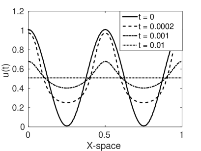
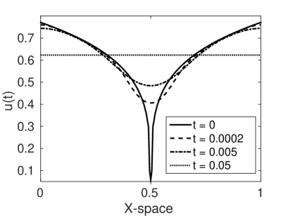
Figure 1. Time evolution of the solution to the diffusion equation (1) with $\alpha=-1$ for two different initial conditions.

A nice feature of the Wasserstein gradient flow scheme is that we may interpret the evolution as a process of redistribution of particles with spatio-temporal density $u(x,t)$ on ${\mathbb{T}}$ under the influence of a nonlinear particle interaction, which is described by $S$. The way in which the initial density $u^{0}$ is “deformed” during the time evolution is illustrated in Figure 2. We have chosen 50 “test particles” for the solutions to (1) for the initial conditions chosen above. We stress the fact that the density of trajectories can generally be not identified with the density $u$ of the solution.

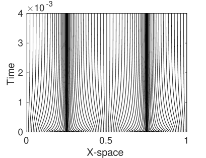
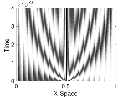
Figure 2. Particle trajectories in the Wasserstein gradient flow scheme, corresponding to the solutions of Figure 1 with $N=50$.

We verify that the discretization is indeed of second order. Figure 3 shows the $\ell^{\infty}$-error for various numbers of grid points $N$. We have chosen the initial datum $u_{0}(x)=\cos(2\pi x)^{2}+0.1$, the end time $T=0.004$, and the time step size $\tau=10^{-7}$. The reference solution is computed by using $N=500$, and $\tau=10^{-7}$. The differences $g(\cdot,T)-g_{\rm ref}(\cdot,T)$ and $u(\cdot,T)-u_{\rm ref}(\cdot,T)$ in the $\ell^{\infty}$ norm feature the expected second-order dependence on $N$.

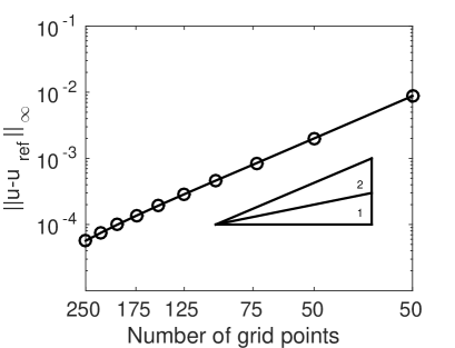
Figure 3. $\ell^{\infty}$-error for $(g-g_{\rm ref})(T)$ (left) and $(u-u_{\rm ref})(T)$ (right) at $T=0.004$ for various numbers of grid points.

Next, we fix the number of grid points $N=100$ and compute the $L^{\infty}(\tau^{*},T;$ $L^{2}({\mathbb{T}}))$ error for varying time step sizes $\tau$; see Figure 4. Because of the approximation of the initial datum as detailed in Section 3.7, the error will be not of second order initially. Therefore, we compute the error in the interval $(\tau^{*},T)$ with $\tau^{*}=10^{-4}$. The errors are of second order, as expected.

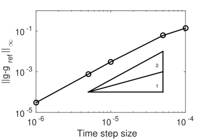
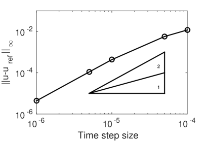
Figure 4. $\ell^{\infty}(\tau^{*},T;\ell^{2}({\mathbb{T}}))$-error for $g-g_{\rm ref}$ (left) and $u-u_{\rm ref}$ (right) for various time step sizes, with $\tau^{*}=10^{-4}$.

The time decay of the discrete version of the relative entropy $S[u]-S[u_{\infty}]$ is presented in Figure 5 (left) for various grid numbers. We observe that the decay is exponential until saturation. The saturation comes from the spatial error and the error from the Newton iteration. The decay rate is estimated in the linear regime from the difference quotient

$$\lambda\approx\frac{1}{\tau}\big{(}\log S[u(t+\tau)]-\log S[u(t)]\big{)}.$$

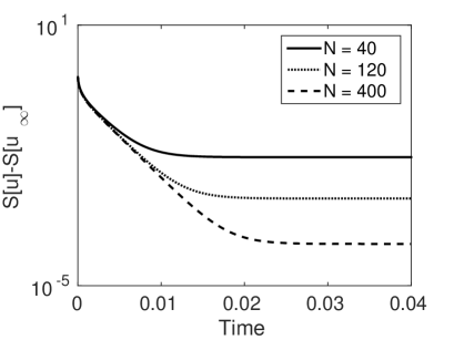
Figure 5. Discrete relative entropy $S[u(t)]-S[u_{\infty}]$ versus time with $\alpha=-1$ for various $N$.

The numerical decay rates for $\alpha=-1,-2$ are shown in Figure 6. The rate for $\alpha=-2$ (right) is much larger than the corresponding one for $\alpha=-1$ (left), since a smaller exponent yields a larger diffusion coefficient (if $u<1$) and thus, diffusion becomes faster. We also see that the decay rates become larger on a finer spatial grid. This behavior seems to confirm recent analytical results for spatial discretizations of Fokker-Planck equations; see [21, Section 5]. One may ask if a similar behavior can be observed for the decay rate as a function of the time step size. However, our numerical experiments do not show a monotonic dependence (figures not presented); rather the decay rates vary in a small range which seems to be determined by the other numerical error parts.

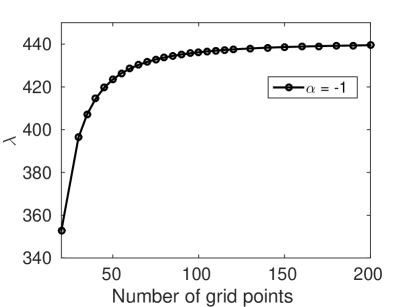
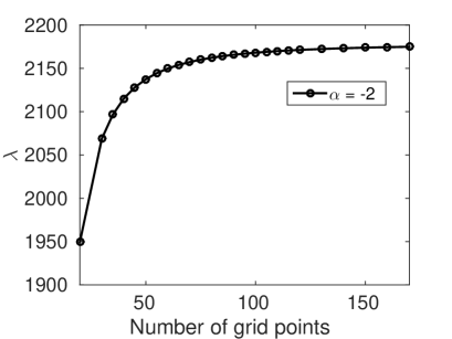
Figure 6. Estimated decay rate of the entropy versus number of grid points $N$ for $\alpha=-1$ (left) and $\alpha=-2$ (right).

In Figure 7, the decay of the square of the relative $G$-norm is presented. The $G$-norm is calculated according to (2), where the argument is given by $\mathbf{g}-\mathbf{g}_{\infty}$ and $\mathbf{g}_{\infty}$ is the weight vector corresponding to the constant steady state. Again, the decay is much faster for $\alpha=-2$ because of the faster diffusion.

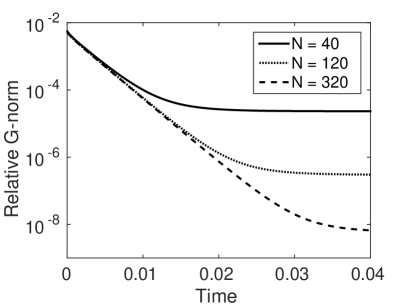
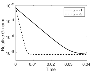
Figure 7. Relative $G$-norm versus time for various grid numbers $N$ (left) and for two values of the exponent $\alpha$ (right).

Finally, we present some results on the time decay of the discrete variance of $u^{n}$ and $g^{n}$ at time $\tau n$, defined by

$$\mbox{Var}(u^{n})^{2}=\sum_{i=1}^{N+1}(u^{n}_{i}-E)^{2}(x_{i}-x_{i-1}),$$

where $E$ is the expectation value of $u^{n}$ (which equals the mass and is therefore constant in time). The discrete variance of $g^{n}$ is defined in a similar way. Interestingly, the variances are exponentially decaying (Figure 8), although it is not clear how to prove this property analytically.

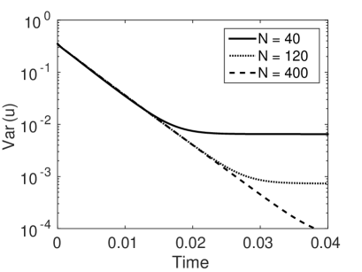
Figure 8. Discrete variance of $u^{n}$ (left) and $g^{n}$ (right) versus time for various grid numbers $N$.

5. Conclusion

We have proposed an extension of the standard minimizing movement scheme to higher-order BDF time discretizations. Quadratic finite elements have been used to discretise in (mass) space. As an example, we have considered a (singular) diffusion equation, but it should be possible to adapt the scheme to other partial differential equations which constitute $L^{2}$ Wasserstein gradient flows. The implicit numerical scheme is based on successive solution of constrained minimization problems. The quadratic convergence in space and time of our method has been confirmed numerically. It turns out that the relative entropy, $G$-norm, and variance converge exponentially to zero. An interesting observation is that the decay rate depends monotonically on the number of grid numbers, but it seems that there is no monotonic behavior with respect to the time step size. Future work may be concerned with an analytical derivation of numerical decay rates using a discrete variant of the Bakry-Emery approach. First steps in this direction were presented in [21] but only for a semi-discretization. Possibly this approach has to be adapted to $G$-stable schemes in the spirit of [18].

Appendix A Proofs of Theorems 1 and 2

Proof of Theorem 1.

The existence proof is based on a regularization of the initial datum and a fixed-point argument. Let $0<\varepsilon<1$ and $u_{0,\varepsilon}=u^{0}+\varepsilon$. Let $Q_{T}={\mathbb{T}}^{d}\times(0,T)$ and $M=\sup_{{\mathbb{T}}^{d}}u^{0}$, Set

$$K=\{u\in L^{2}(Q_{T}):\varepsilon\leq u\leq M,\ \|u\|_{L^{2}(0,T;H^{1}({\mathbb{T}}^{d}))}+\|\partial_{t}u\|_{L^{2}(0,T;H^{1}({\mathbb{T}}^{d})^{\prime})}\leq C\},$$

where $C>0$ will be determined later. The set $K$ is convex and, by Aubin’s lemma, compact in $L^{2}(Q_{T})$. Let $v\in K$ and let $u\in L^{2}(Q_{T})$ be the weak solution to

(18) $$\partial_{t}u=\mbox{\rm div}(v^{\alpha-1}\nabla u)\quad\mbox{in }{\mathbb{T}}^{d},\ t>0,\quad u(0)=u_{0,\varepsilon}.$$

This defines the fixed-point operator $Z:K\to L^{2}(Q_{T})$, $v\mapsto u$. Standard arguments show that $Z$ is continuous. We verify that $Z(K)\subset K$. By the maximum principle, $\varepsilon\leq u\leq M$. Using $u$ as a test function in the weak formulation of (18) shows that $\|u\|_{L^{2}(0,T;H^{1}({\mathbb{T}}^{d}))}\leq C_{1}(\varepsilon)$, where $C_{1}(\varepsilon)>0$ is some constant depending on $\varepsilon$. Moreover, $\|\partial_{t}u\|_{L^{2}(0,T;H^{1}({\mathbb{T}}^{d})^{\prime})}\leq\|v^{\alpha-1}\nabla u\|_{L^{2}(Q_{T})}\leq C_{2}(\varepsilon)$. Thus, setting, $C:=C_{1}(\varepsilon)+C_{2}(\varepsilon)$, we infer that $u\in K$. By the fixed-point theorem of Schauder, there exists a fixed point $u_{\varepsilon}$ of $Z$.

In order to perform the limit $\varepsilon\to 0$, we need to derive $\varepsilon$-independent estimates for $u_{\varepsilon}$. To this end, we need to distinguish several cases. First, let $\alpha=-1$. Employing the test function $1-1/u_{\varepsilon}$ in the weak formulation of (18) with $u=v=u_{\varepsilon}$, we find that

$$\int_{{\mathbb{T}}^{d}}(u_{\varepsilon}(t)-\log u_{\varepsilon}(t))\,dx+\int_{0}^{t}\int_{{\mathbb{T}}^{d}}|\nabla u_{\varepsilon}^{-1}|^{2}\,dxds=\int_{{\mathbb{T}}^{d}}(u^{0}+\varepsilon-\log(u^{0}+\varepsilon))\,dx.$$

The right-hand side is uniformly bounded as we assumed that $-\int_{{\mathbb{T}}^{d}}\log u^{0}\,dx<\infty$. Since $|\nabla u_{\varepsilon}^{-1}|^{2}\geq M^{-4}|\nabla u_{\varepsilon}|^{2}$, we infer uniform estimates for $u_{\varepsilon}$ in $L^{2}(0,T;H^{1}({\mathbb{T}}^{d}))$ and also in $H^{1}(0,T;H^{1}({\mathbb{T}}^{d})^{\prime})$.

Next, let $\alpha\neq-1$. The test function $u_{\varepsilon}^{\alpha}$ in the weak formulation of (18) gives

$$\frac{1}{\alpha+1}\int_{{\mathbb{T}}^{d}}u_{\varepsilon}(t)^{\alpha+1}\,dx+\frac{1}{\alpha}\int_{0}^{t}\int_{{\mathbb{T}}^{d}}|\nabla u_{\varepsilon}^{\alpha}|^{2}\,dxds=\frac{1}{\alpha+1}\int_{{\mathbb{T}}^{d}}(u^{0}+\varepsilon)^{\alpha+1}\,dx,$$

If $-1<\alpha<0$, we write this equation as

$$\int_{0}^{t}\int_{{\mathbb{T}}^{d}}|\nabla u_{\varepsilon}^{\alpha}|^{2}\,dxds =-\frac{\alpha}{\alpha+1}\int_{{\mathbb{T}}^{d}}u_{\varepsilon}(t)^{\alpha+1}\,dx+\frac{\alpha}{\alpha+1}\int_{{\mathbb{T}}^{d}}(u^{0}+\varepsilon)^{\alpha+1}\,dx$$

$$\leq-\frac{\alpha}{\alpha+1}\int_{{\mathbb{T}}^{d}}M^{\alpha+1}\,dx.$$

If $\alpha<-1$, we obtain

$$\frac{1}{-\alpha-1}\int_{{\mathbb{T}}^{d}}u_{\varepsilon}(t)^{\alpha+1}\,dx+\frac{1}{-\alpha}\int_{0}^{t}\int_{{\mathbb{T}}^{d}}|\nabla u_{\varepsilon}^{\alpha}|^{2}\,dxds=\frac{1}{-\alpha-1}\int_{{\mathbb{T}}^{d}}(u^{0}+\varepsilon)^{\alpha+1}\,dx.$$

In both cases, since $u^{0}$ is assumed to be bounded, we infer a uniform bound for $u_{\varepsilon}^{\alpha}$ in $L^{2}(0,T;H^{1}({\mathbb{T}}^{d}))$ and consequently also for $\partial_{t}u_{\varepsilon}$ in $L^{2}(0,T;H^{1}({\mathbb{T}}^{d})^{\prime})$. Moreover, in view of $|\nabla u_{\varepsilon}^{\alpha}|^{2}=\alpha^{2}u_{\varepsilon}^{2(\alpha-1)}|\nabla u_{\varepsilon}|^{2}\geq\alpha^{2}M^{2(\alpha-1)}|\nabla u_{\varepsilon}|^{2}$, it follows that $(u_{\varepsilon})$ is bounded in $L^{2}(0,T;H^{1}({\mathbb{T}}^{d}))$.

We infer for all $\alpha<0$ the following bounds:

$$\|u_{\varepsilon}\|_{L^{\infty}(0,T;L^{\infty}({\mathbb{T}}^{d}))}+\|u_{\varepsilon}^{\alpha}\|_{L^{2}(0,T;H^{1}({\mathbb{T}}^{d}))}+\|u_{\varepsilon}\|_{L^{2}(0,T;H^{1}({\mathbb{T}}^{d}))}+\|\partial_{t}u_{\varepsilon}\|_{L^{2}(0,T;H^{1}({\mathbb{T}}^{d})^{\prime})}\leq C_{3}.$$

By Aubin’s lemma, there exists a subsequence which is not relabeled such that $u_{\varepsilon}\to u$ strongly in $L^{2}(Q_{T})$ as $\varepsilon\to 0$. Moreover, $u_{\varepsilon}^{\alpha}\rightharpoonup u^{\alpha}$ weakly in $L^{2}(0,T;H^{1}({\mathbb{T}}^{d}))$ and $\partial_{t}u_{\varepsilon}\rightharpoonup\partial_{t}u$ weakly in $L^{2}(0,T;H^{1}({\mathbb{T}}^{d})^{\prime})$. Thus, we may pass to the limit $\varepsilon\to 0$ in the weak formulation which shows that $u$ solves (1). ∎

Proof of Theorem 2.

Employing (1) and integration by parts, we find that

$$\frac{dH_{\beta}}{dt}=-\beta(\beta-1)\int_{{\mathbb{T}}^{d}}u^{\alpha+\beta-3}|\nabla u|^{2}\,dx=-\frac{4}{\beta}(\beta-1)\int_{{\mathbb{T}}^{d}}u^{\alpha-1}|\nabla u^{\beta/2}|^{2}\,dx.$$

We employ the bound $u\leq M=\sup_{{\mathbb{T}}^{d}}u^{0}$ and the Beckner inequality [3] (note that we assumed that $\mbox{vol}({\mathbb{T}}^{d})=1$),

(19) $$\int_{{\mathbb{T}}^{d}}u^{\beta}\,dx-\bigg{(}\int_{{\mathbb{T}}^{d}}u\,dx\bigg{)}^{\beta}\leq C_{B}\int_{{\mathbb{T}}^{d}}|\nabla u^{\beta/2}|^{2}\,dx\quad\mbox{for }u^{\beta/2}\in H^{1}(\Omega),\ 1<\beta\leq 2,$$

to obtain

$$\frac{dH_{\beta}}{dt}\leq-\frac{4(\beta-1)}{\beta C_{B}}M^{\alpha-1}\bigg{(}\int_{{\mathbb{T}}^{d}}u^{\beta}\,dx-\bigg{(}\int_{{\mathbb{T}}^{d}}u\,dx\bigg{)}^{\beta}\bigg{)}=-\frac{4(\beta-1)}{\beta C_{B}}M^{\alpha-1}H_{\beta}.$$

Then Gronwall’s lemma yields $H[u(t)]\leq H[u^{0}]e^{-\lambda t}$ with $\lambda=-4(\beta-1)M^{\alpha-1}/(\beta C_{B})$ for $1<\beta\leq 2$.

For the second result, let $-1\leq\alpha<0$ and $\beta=2(1-\alpha)$. Similarly as above, we find that

$$\frac{dH_{\beta}}{dt} =-\frac{4\beta(\beta-1)}{(\alpha+\beta-1)^{2}}\int_{{\mathbb{T}}^{d}}|\nabla u^{(\alpha+\beta-1)/2}|^{2}\,dx$$

$$\leq-\frac{8(1-2\alpha)}{1-\alpha}\int_{{\mathbb{T}}^{d}}\bigg{(}\int_{{\mathbb{T}}^{d}}u^{\alpha+\beta-1}\,dx-\bigg{(}\int_{{\mathbb{T}}^{d}}u\,dx\bigg{)}^{\alpha+\beta-1}\bigg{)}$$

$$=-\frac{8(1-2\alpha)}{1-\alpha}H_{\beta/2}[u],$$

since $\alpha+\beta-1=\beta/2\in(1,2]$. Using the inequalities $\|u^{\beta/2}\|_{L^{2}({\mathbb{T}}^{d})}\geq\|u^{\beta/2}\|_{L^{1}({\mathbb{T}}^{d})}$ and $\|u^{\beta/2}\|_{L^{2}({\mathbb{T}}^{d})}=\|u\|_{L^{\beta}({\mathbb{T}}^{d})}^{\beta/2}\geq\|u\|_{L^{1}({\mathbb{T}}^{d})}^{\beta/2}$ (again we employ $\mbox{vol}({\mathbb{T}}^{d})=1$ here), it follows that

$$H_{\beta}[u] =\|u^{\beta/2}\|_{L^{2}({\mathbb{T}}^{d})}^{2}-\|u\|_{L^{1}({\mathbb{T}}^{d})}^{\beta}$$

$$=\big{(}\|u^{\beta/2}\|_{L^{2}({\mathbb{T}}^{d})}+\|u\|_{L^{1}({\mathbb{T}}^{d})}^{\beta/2}\big{)}\big{(}\|u^{\beta/2}\|_{L^{2}({\mathbb{T}}^{d})}-\|u\|_{L^{1}({\mathbb{T}}^{d})}^{\beta/2}\big{)}$$

$$\geq\big{(}\|u^{\beta/2}\|_{L^{2}({\mathbb{T}}^{d})}+\|u\|_{L^{1}({\mathbb{T}}^{d})}^{\beta/2}\big{)}\big{(}\|u^{\beta/2}\|_{L^{1}({\mathbb{T}}^{d})}-\|u\|_{L^{1}({\mathbb{T}}^{d})}^{\beta/2}\big{)}$$

$$\geq\big{(}\|u^{\beta/2}\|_{L^{1}({\mathbb{T}}^{d})}+\|u\|_{L^{1}({\mathbb{T}}^{d})}^{\beta/2}\big{)}H_{\beta/2}[u]\geq 2\|u\|_{L^{1}({\mathbb{T}}^{d})}^{\beta/2}H_{\beta/2}[u].$$

Since the solution to (1) conserves mass, $\|u(t)\|_{L^{1}({\mathbb{T}}^{d})}=\|u^{0}\|_{L^{1}({\mathbb{T}}^{d})}$, and we end up with

$$\frac{dH_{\beta}}{dt}\leq-\frac{4(1-2\alpha)}{(1-\alpha)\|u^{0}\|_{L^{1}({\mathbb{T}}^{d})}^{\beta/2}}H_{\beta}[u].$$

Then Gronwall’s lemma shows that $H_{\beta}[u(t)]\leq H_{\beta}[u^{0}]e^{-\lambda t}$ with $\lambda=4(1-2\alpha)/((1-\alpha)\|u^{0}\|_{L^{1}({\mathbb{T}}^{d})}^{1-\alpha})$.

Finally, the statement of the theorem follows after applying the generalized Csiszár-Kullback inequality in the form

$$\|u-v\|_{L^{1}({\mathbb{T}}^{d})}^{2}\leq C_{\beta}\|v\|_{L^{1}({\mathbb{T}}^{d})}\bigg{(}\int_{{\mathbb{T}}^{d}}u^{\beta}-\bigg{(}\int_{{\mathbb{T}}^{d}}u\,dx\bigg{)}^{\beta}\bigg{)},\quad 1<\beta\leq 2.$$

for functions $u$, $v\in L^{\beta}({\mathbb{T}}^{d})$ such that $\int_{{\mathbb{T}}^{d}}u\,dx=\int_{{\mathbb{T}}^{d}}v\,dx$. The proof is a slight generalization of the proof of Theorem 1.4 in [16] taking $\varphi(t)=t^{\beta}$. ∎

Appendix B Computations

In this appendix, we detail the calculations for the coefficients of the matrix (13), and the Hessian of the discrete entropy (16), both in the case $\alpha=-1$.

B.1. Computation of the coefficients $M_{ij}$

We compute the coefficients of the matrix (14), i.e. the coefficients $a_{ij}$, $b_{ij}$, and $c_{ij}$ defined in (13). In the following, we set

$$\delta_{j}=\omega_{j}-\omega_{j-1},\quad\Delta_{j}=\frac{1}{2}(\omega_{j+1}-\omega_{j-1}),\quad\sigma_{j}=\frac{1}{3}(\omega_{j+1}+\omega_{j}+\omega_{j-1}).$$

Lemma 4 (Coefficients $a_{ij}$).

The coefficients of the symmetric matrix $A=(a_{ij})$, defined in (13), read as

$$a_{jj} =\Delta_{j}^{2}(M-\sigma_{j})-\frac{\Delta_{j}}{60}(12\Delta_{j}^{1}+\delta_{j}^{2}+\delta_{j+1}^{2}),\quad 1\leq j\leq N-1,$$

$$a_{j,j+1} =\Delta_{j}\Delta_{j+1}(M-\sigma_{j+1})-\frac{\delta_{j}^{3}}{120},\quad 1\leq j\leq N-1,$$

$$a_{jk} =\Delta_{j}\Delta_{k}(M-\sigma_{k}),\quad j+2\leq k\leq N-1,$$

$$a_{1N} =\frac{1}{2}\Delta_{1}\Delta_{N}\bigg{(}M-\frac{\omega_{2}}{3}\bigg{)}-\frac{\Delta_{N}^{3}}{120},$$

$$a_{jN} =\frac{1}{2}\Delta_{j}\Delta_{N}\bigg{(}M-\sigma_{j}+\frac{\delta_{N}}{3}\bigg{)},\quad 2\leq j\leq N-2,$$

$$a_{N-1,N} =\frac{1}{2}\Delta_{N-1}\Delta_{N}\bigg{(}M-\frac{1}{3}(\omega_{N-2}+2\omega_{N-1})\bigg{)}-\frac{\Delta_{N}^{3}}{120},$$

$$a_{NN} =\frac{M}{4}\Delta_{N}^{2}+\frac{\Delta_{N}^{3}}{10}.$$

This lemma was proved in [13, Lemma 2.6]. For the convenience of the reader, we recall the proof below.

Proof.

We reformulate the integral in (13):

$$a_{jk}=M\int_{0}^{M}\phi_{j}(\eta)\,d\eta\int_{0}^{M}\phi_{k}(\eta^{\prime})\,d\eta^{\prime}-\int_{0}^{M}\phi_{j}(\eta)\,d\eta\int_{0}^{M}\eta^{\prime}\phi_{k}(\eta^{\prime})\,d\eta^{\prime}-J_{jk},$$

$$\mbox{where }J_{jk}=\int_{0}^{M}\int_{0}^{M}(\eta-\eta^{\prime})_{+}\phi_{j}(\eta)\phi_{k}(\eta^{\prime})\,d\eta d\eta^{\prime},$$

where $(\eta-\eta^{\prime})_{+}:=\max\{0,\eta-\eta^{\prime}\}$. The first two integrals become

$$\int_{0}^{m}\phi_{j}(\eta)\,d\eta=\delta_{j},\quad\int_{0}^{M}\eta^{\prime}\phi_{k}(\eta^{\prime})\,d\eta^{\prime}=\Delta_{k}\sigma_{k}.$$

Since $A$ is symmetric, it is sufficient to consider $1\leq j\leq k$. If $j+2\leq k<N$, the support of $\phi_{j}(\eta)\phi_{k}(\eta^{\prime})$ is contained in $[\omega_{j-1},\omega_{j+1}]\times[\omega_{k-1}\times\omega_{k+1}]$. Hence, the support is nonvanishing if $\eta\leq\omega_{j+1}\leq\omega_{k-1}\leq\eta^{\prime}$, but then $(\eta-\eta^{\prime})_{+}=0$ except for $\eta=\eta^{\prime}$. We conclude that $J_{jk}=0$ and it is sufficient to compute only $J_{jj}$ and $J_{j,j+1}$:

$$J_{jj} =\int_{\omega_{j-1}}^{\omega_{j+1}}\phi_{j}(\eta)\bigg{(}\int_{\omega_{j-1}}^{\eta}(\eta-\eta^{\prime})\phi_{j}(\eta^{\prime})\,d\eta^{\prime}\bigg{)}\,d\eta=\frac{\Delta_{j}}{60}(12\Delta_{j}^{2}+\delta_{j}^{2}+\delta_{j+1}^{2}),$$

$$J_{j,j+1} =\int_{\omega_{j-1}}^{\omega_{j+1}}\phi_{j}(\eta)\bigg{(}\int_{\omega_{j-1}}^{\max\{\eta,\omega_{j}\}}(\eta-\eta^{\prime})\phi_{j}(\eta^{\prime})\,d\eta^{\prime}\bigg{)}\,d\eta=\frac{\delta_{j}^{3}}{120}.$$

Next, let $k=N$. Then the support of $\phi_{N}$ is contained in $[0,\omega_{1}]\cup[\omega_{N-1},M]$, and we compute:

$$a_{jN} =M\int_{0}^{M}\phi_{j}(\eta)\,d\eta\int_{0}^{M}\phi_{N}(\eta^{\prime})\,d\eta^{\prime}-\int_{0}^{M}\eta\phi_{j}(\eta)\,d\eta\int_{0}^{\omega_{1}}\phi_{N}(\eta^{\prime})\,d\eta^{\prime}$$

$$\phantom{xx}{}-\int_{0}^{M}\phi_{j}(\eta)\,d\eta\int_{\omega_{N-1}}^{M}\eta^{\prime}\phi_{N}(\eta^{\prime})\,d\eta^{\prime}-K_{j}^{+}-K_{j}^{-}$$

$$=\frac{1}{2}\Delta_{j}\Delta_{N}\bigg{(}M-\sigma_{j}+\frac{\delta_{N}}{3}\bigg{)}-K_{j}^{+}-K_{j}^{-},$$

where

$$K_{j}^{+} :=\int_{0}^{M}\int_{\eta}^{\omega_{1}}(\eta^{\prime}-\eta)_{+}\phi_{j}(\eta)\phi_{N}(\eta^{\prime})\,d\eta d\eta^{\prime},$$

$$K_{j}^{-} :=\int_{0}^{M}\int_{\omega_{N-1}}^{M}(\eta-\eta^{\prime})_{+}\phi_{j}(\eta)\phi_{N}(\eta^{\prime})\,d\eta d\eta^{\prime}.$$

For $2\leq j\leq N-2$, the supports of $\phi_{j}$ and $\phi_{N}$ do not intersect such that $K_{j}^{\pm}=0$. For $j=1$, we have $K_{1}^{-}=0$ and $K_{1}^{+}=\Delta_{N}^{3}/120$, whereas for $j=N-1$, $K_{N-1}^{+}=0$ and $K_{N-1}^{-}=\Delta_{N}^{3}/120$. Furthermore, $K_{N}^{\pm}=\Delta_{N}^{3}/30$. Moreover, since $\delta_{N}=\omega_{N}-\omega_{N-1}=(M-\omega_{0})-(M-\omega_{1})=\omega_{1}$,

$$M-\sigma_{1}+\frac{\delta_{N}}{3}=M-\frac{1}{3}(\omega_{0}+\omega_{1}+\omega_{2})+\frac{1}{3}\omega_{1}=M-\frac{\omega_{2}}{3}.$$

Collecting these results, the lemma follows. ∎

Lemma 5 (Coefficients $b_{ij}$).

The coefficients of the matrix $B=(b_{ij})$, defined in (13), read as

$$b_{jj} =\frac{2}{3}\delta_{j}(M\Delta_{j}-\delta_{j}\sigma_{j})+\beta_{jj},\quad 1\leq j\leq N,$$

$$b_{j+1,j} =\frac{1}{3}\big{(}2M\delta_{j+1}\Delta_{j}-(\omega_{j+2}^{2}-\omega_{j+1}^{2})\Delta_{j}\big{)}+\beta_{j+1,j},\quad 1\leq j\leq N-1,$$

$$b_{jk} =\frac{2}{3}(M\delta_{j}\Delta_{k}-\delta_{j}\delta_{k}\sigma_{k}),\quad 1\leq j<k\leq N,$$

$$b_{jk} =\frac{1}{3}\big{(}2M\delta_{j}\Delta_{k}-(\omega_{j+1}^{2}-\omega_{j}^{2})\Delta_{k}\big{)},\quad j\geq k-2,$$

$$b_{1N} =\frac{2}{3}\delta_{1}\Delta_{N}-\frac{1}{6}(\omega_{2}^{2}-\omega_{1}^{2})\delta_{N}-\frac{1}{9}(2\omega_{N}^{2}-\omega_{N-1}^{2}-\omega_{N-1}\omega_{N})\delta_{1}-\beta_{1N},$$

$$b_{jN} =\frac{2}{3}\delta_{j}\Delta_{N}-\frac{1}{6}(\omega_{j+1}^{2}-\omega_{j}^{2})\delta_{N}-\frac{1}{9}(2\omega_{N}^{2}-\omega_{N-1}^{2}-\omega_{N-1}\omega_{N})\delta_{j},\quad 2\leq j\leq N-1,$$

$$b_{NN} =\frac{2}{3}\delta_{N}\Delta_{N}-\frac{1}{6}(\omega_{N}^{2}-\omega_{N-1}^{2})\delta_{N}-\frac{1}{9}(2\omega_{N}^{2}-\omega_{N-1}^{2}-\omega_{N-1}\omega_{N})\delta_{N}-\beta_{NN},$$

where

$$\beta_{jj} =-\frac{1}{45}\omega_{j+1}^{2}+\frac{1}{90}\omega_{j+1}^{2}\omega_{j}+\frac{1}{18}\omega_{j+1}^{2}\omega_{j+2}-\frac{1}{15}\omega_{j+1}\omega_{j}^{2}+\frac{1}{9}\omega_{j+2}\omega_{j+1}\omega_{j}$$

$$\phantom{xx}{}-\frac{1}{9}\omega_{j+2}^{2}\omega_{j+1}+\frac{7}{90}\omega_{j}^{3}-\frac{1}{6}\omega_{j}^{2}\omega_{j+2}+\frac{1}{9}\omega_{j}\omega_{j+2}^{2},$$

$$\beta_{j+1,j} =\frac{1}{45}\left(\omega_{j+2}^{3}-\omega_{j+1}^{3}+3(\omega_{j+1}^{2}\omega_{j+2}-\omega_{j+2}^{2}\omega_{j+1})\right),$$

$$\beta_{1N} =\frac{1}{45}\big{(}\omega_{2}^{2}-\omega_{1}^{2}+3(\omega_{2}\omega_{1}^{2}-\omega_{2}^{2}\omega_{1})\big{)},$$

$$\beta_{NN} =\frac{1}{45}\big{(}\omega_{N+1}^{3}-\omega_{N}^{3}+3(\omega_{N}^{2}\omega_{N+1}-\omega_{N+1}^{2}\omega_{N})\big{)}.$$

Proof.

The computation is similar to the previous proof. We write the integral for $b_{jk}$ with $j$, $k\leq N-1$ and for $j<k$ as

$$b_{jk}=M\int_{0}^{M}\phi_{N+j}(\eta)\,d\eta\int_{0}^{M}\phi_{k}(\eta^{\prime})\,d\eta^{\prime}-\int_{0}^{M}\phi_{N+j}(\eta)\,d\eta\int_{0}^{M}\eta^{\prime}\phi_{k}(\eta^{\prime})\,d\eta^{\prime}-J^{-}_{jk},$$

and for $j>k$ as

$$b_{jk}=M\int_{0}^{M}\phi_{N+j}(\eta)\,d\eta\int_{0}^{M}\phi_{k}(\eta^{\prime})\,d\eta^{\prime}-\int_{0}^{M}\eta\phi_{N+j}(\eta)\,d\eta\int_{0}^{M}\phi_{k}(\eta Ä)\,d\eta^{\prime}-J^{+}_{jk},$$

where

$$J^{-}_{jk}=\int_{0}^{M}\int_{0}^{M}(\eta-\eta^{\prime})_{+}\phi_{N+j}(\eta)\phi_{k}(\eta^{\prime})\,d\eta d\eta^{\prime},$$

$$J^{+}_{jk}=\int_{0}^{M}\int_{0}^{M}(\eta^{\prime}-\eta)_{+}\phi_{N+j}(\eta)\phi_{k}(\eta^{\prime})\,d\eta d\eta^{\prime}.$$

We compute

$$\int_{0}^{M}\phi_{N+j}(\eta)\,d\eta=\frac{2}{3}\delta_{j},\quad\int_{0}^{M}\eta\phi_{N+j}(\eta)\,d\eta=\frac{1}{3}(\omega_{j+1}^{2}-\omega_{j}^{2}).$$

The integrals $J^{\pm}_{jk}$ vanish if $k\neq j-1,j$ since $(\eta-\eta^{\prime})_{+}$ and $(\eta^{\prime}-\eta)_{+}$ vanish. This proves the expressions for $b_{jk}$ with $j\leq k-1$ and $j\geq k+2$. The coefficients $b_{jj}$ and $b_{j+1,j}$ are calculated in the same way.

It remains to compute the matrix coefficients coming from the boundary elements. The computation of $b_{jN}$ is straightforward as the support of $\phi_{2N}$ is contained on the single subinterval $[\omega_{N-1},M]$. For the boundary elements $b_{jN}$, we take into account that the support of $\phi_{N}$ is contained in $[\omega_{N-1},M]$ and $[0,\omega_{1}]$, which yields

$$b_{jN} =M\int_{0}^{M}\phi_{N+j}(\eta)\,d\eta\int_{0}^{M}\phi_{N}(\eta^{\prime})\,d\eta^{\prime}-\int_{0}^{M}\eta\phi_{N+j}(\eta)\,d\eta\int_{0}^{\omega_{1}}\phi_{N}(\eta^{\prime})\,d\eta^{\prime}-\beta_{1N}-\beta_{NN},$$

where

$$\beta_{1N} =\int_{0}^{M}\int_{0}^{\omega_{1}}(\eta^{\prime}-\eta)_{+}\phi_{N+j}(\eta)\phi_{N}(\eta^{\prime})\,d\eta d\eta^{\prime},$$

$$\beta_{NN} =\int_{0}^{M}\int_{\omega_{N-1}}^{M}(\eta-\eta^{\prime})_{+}\phi_{j}(\eta)\phi_{N}(\eta^{\prime})\,d\eta d\eta^{\prime},$$

and the computation is as before. ∎

Lemma 6 (Coefficients $c_{ij}$).

The coefficients of the symmetric matrix $C=(c_{ij})$, defined in (13), read as

$$c_{jj} =\frac{8}{9}\delta_{j}^{2}-\frac{2}{9}\delta_{j}(\omega_{j+1}^{2}-\omega_{j}^{2})-\frac{2}{35}\big{(}\omega_{j+1}^{3}-\omega_{j}^{3}-3\omega_{j+1}\omega_{j}(\omega_{j+1}-\omega_{j})\big{)},\quad 1\leq j\leq N,$$

$$c_{jk} =\frac{8}{9}\delta_{j}\delta_{k}-\frac{2}{9}\delta_{j}(\omega_{k+1}^{2}-\omega_{k}^{2}),\quad 1\leq j<k\leq N.$$

Proof.

We compute

$$c_{jk}=M\int_{0}^{M}\phi_{N+j}(\eta)\,d\eta\int_{0}^{M}\phi_{N+k}(\eta^{\prime})\,d\eta^{\prime}-\int_{0}^{M}\phi_{N+j}(\eta)\,d\eta\int_{0}^{M}\eta^{\prime}\phi_{N+k}(\eta^{\prime})\,d\eta^{\prime}-\gamma_{jk},$$

$$\mbox{where }\gamma_{jk}=\int_{0}^{M}\int_{0}^{M}(\eta-\eta^{\prime})_{+}\phi_{N+j}(\eta)\phi_{N+k}(\eta^{\prime})\,d\eta d\eta^{\prime}.$$

As before, we find that $\gamma_{jk}=0$ for all $j\neq k$. Moreover,

$$\gamma_{jj}=\int_{\omega_{j-1}}^{\omega_{j}}\phi_{N+j}(\eta)\,d\eta\int_{\omega_{j}}^{\eta}(\eta-\eta^{\prime})\phi_{N+j}(\eta^{\prime})\,d\eta^{\prime}=\frac{2}{35}\big{(}\omega_{j+1}^{3}-\omega_{j}^{3}-3(\omega_{j+1}\omega_{j}(\omega_{j+1}-\omega_{j})\big{)},$$

which finishes the proof. ∎

B.2. Computation of the coefficients of the Hessian of $S_{N}$

We compute the gradient and Hessian of the discrete entropy (16) for the case $\alpha=-1$. We set for $k=0,\ldots,N-1$:

$$S_{N,k}[{\mathbf{g}}]=\frac{1}{2}\int_{\omega_{k}}^{\omega_{k+1}}\big{(}g_{k}\phi_{k}(\omega)+g_{k+1}\phi_{k+1}(\omega)+g_{N+k}\phi_{N+k}(\omega)\big{)}\,d\omega,$$

where ${\mathbf{g}}=(g_{1},\ldots,g_{2N})\in{\mathbb{G}}_{M}^{N}$. Furthermore, we abbreviate $\partial_{k}S_{N,j}=\partial S_{N,j}/\partial g_{k}$ and $\partial_{j,k}S_{N,\ell}=\partial S_{N,\ell}/\partial g_{j}\partial_{k}g$. A computation shows that

$$\partial_{k}S_{N,k}[{\mathbf{g}}] =\frac{\delta_{k+3}}{3}\big{(}2(g_{N+k}+g_{k})+g_{k+1}\big{)},$$

$$\partial_{k}S_{N,k-1}[{\mathbf{g}}] =\frac{2}{3}\delta_{k}(g_{k}-g_{k-1}-g_{N+k-1}),$$

$$\partial_{N+k}S_{N,k}[{\mathbf{g}}] =\delta_{k+1}\bigg{(}(g_{k+1}+g_{k})+\frac{8}{5}g_{N+k}\bigg{)}.$$

As $S_{N,k}$ and $S_{N,k-1}$ depend on $g_{k}$, we obtain (recall (16))

$$\partial_{k}S_{N}=\partial_{k}S_{N,k}+\partial_{k}S_{N,k-1},\quad\partial_{N+k}S_{N}=\partial_{N+k}S_{N,N+k}.$$

The second-order derivatives become

$$\partial_{k,k-1}S_{N,k-1} =-\frac{2}{3}\delta_{k}, \partial_{k,k}S_{N,k-1} =\frac{2}{3}\delta_{k}, \partial_{k,k}S_{N,k} =-\frac{2}{3}\delta_{k+1},$$

$$\partial_{k,k+1}S_{N,k} =\frac{1}{3}\delta_{k+1}, \partial_{k,N+k-1}S_{N,k-1} =-\frac{2}{3}\delta_{k}, \partial_{k,N+k}S_{N,k} =\frac{2}{3}\delta_{k+1},$$

$$\partial_{N+k,k+1}S_{N,k} =\frac{2}{3}\delta_{k+1}, \partial_{N+k,N+k}S_{N,k} =\frac{16}{15}\delta_{k+1}.$$

Then the elements of the Hessian of $S_{N}$ read as

$$\partial_{k,k-1}S_{N} =\partial_{k,k-1}S_{N,k-1}, \partial_{k,k}S_{N} =\partial_{k,k}S_{N,k}+\partial_{k,k}S_{N,k-1},$$

$$\partial_{k,k+1}S_{N} =\partial_{k,k+1}S_{N,k}, \partial_{k,N+k}S_{N} =\partial_{k,N+k}S_{N,k},$$

$$\partial_{k,N+k-1}S_{N} =\partial_{k,N+k-1}S_{N,k-1}, \partial_{N+k,k+1}S_{N} =\partial_{N+k,k+1}S_{N,k},$$

$$\partial_{N+k,N+k}S_{N} =\partial_{N+k,N+k}S_{N,k}.$$

References

- [1] M. Agueh and M. Bowles. One-dimensional numerical algorithms for gradient flows in the -Wasserstein spaces. Acta Appl. Math. 125 (2013), 121-134.
- [2] L. Ambrosio, N. Gigli, and G. Savaré, Gradient Flows in Metric Spaces and in the Space of Probability Measures. Birkhäuser, Basel, 2005.
- [3] W. Beckner. A generalized Poincaré inequality for Gaussian measures. Proc. Amer. Math. Soc. 105 (1989), 397-400.
- [4] A. Blanchet, V. Calvez, and J. A. Carrillo. Convergence of the mass-transport steepest descent scheme for the subcritical Patlak-Keller-Segel model. SIAM J. Numer. Anal. 46 (2008), 691-721.
- [5] M. Bonforte, J. Dolbeault, G. Grillo, and J. L. Vázquez. Sharp rates of decay of solutions to the nonlinear fast diffusion equation via functional inequalities. Proc. Natl. Acad. Sci. USA 107 (2010), 16459-16464.
- [6] C. Budd, M. Cullen, and E. Walsh. Monge-Ampère based moving mesh methods for numerical weather prediction, with applications to the Eady problem. J. Comput. Phys. 236 (2013), 247-270.
- [7] M. Burger, J. A. Carrillo, and M.-T. Wolfram. A mixed finite element method for nonlinear diffusion equations. Kinetic Related Models 3 (2010), 5983.
- [8] M. Burger, M. Franeka, and C.-B. Schönlieb. Regularised regression and density estimation based on optimal transport. Appl. Math. Res. Express 2 (2012), 209-253.
- [9] J. A. Carrillo, A. Chertock, and Y. Huang. A finite-volume method for nonlinear nonlocal equations with a gradient flow structure. Commun. Comput. Phys. 17 (2015), 233-258.
- [10] J. A. Carrillo, R. McCann, and C. Villani. Contractions in the 2-Wasserstein length space and thermalization of granular media. Arch. Rational Mech. Anal. 179 (2006), 217-263.
- [11] J. A. Carrillo and J. Moll. Numerical simulation of diffusive and aggregation phenomena in nonlinear continuity equations by evolving diffeomorphisms. SIAM J. Sci. Comput. 31 (2009/10), 4305-4329.
- [12] E. De Giorgi, New problems on minimizing movements. In: C. Baiocchi and J.-L. Lions (eds.), Boundary Value Problems for PDE and Applications, pp. 81-98. Masson, Paris, 1993.
- [13] B. Düring, D. Matthes, and J.-P. Milišić. A gradient flow scheme for nonlinear fourth order equations. Discrete Cont. Dyn. Sys. B 14 (2010), 935-959.
- [14] U. Gianazza, G. Savaré, and G. Toscani. The Wasserstein gradient flow of the Fisher information and the quantum drift-diffusion equation. Arch. Rational Mech. Anal. 194 (2009), 133-220.
- [15] L. Gosse and G. Toscani. Identification of asymptotic decay to self-similarity for one-dimensional filtration equations. SIAM J. Numer. Anal. 43 (2006), 2590-2606.
- [16] N. Gozlan and C. Léonard. Transport inequalities. A survey. Markov Processes Related Fields 16 (2010), 635-736.
- [17] R. Jordan, D. Kinderlehrer, and F. Otto. The variational formulation of the Fokker-Planck equation. SIAM J. Math. Anal. 29 (1998), 1-17.
- [18] A. Jüngel and J.-P. Milišić. Entropy dissipative one-leg multistep time approximations of nonlinear diffusive equations. Numer. Meth. Part. Diff. Eqs. 31 (2015), 1119-1149.
- [19] D. Kinderlehrer and N. Walkington. Approximation of parabolic equations using the Wasserstein metric. ESAIM Math. Model. Numer. Anal. 33 (1999), 837-852.
- [20] D. Matthes and H. Osberger. Convergence of a variational Lagrangian scheme for a nonlinear drift diffusion equation. ESAIM Math. Model. Numer. Anal. 48 (2014), 697-726.
- [21] A. Mielke. Geodesic convexity of the relative entropy in reversible Markov chains. Calc. Var. 48 (2013), 1-31.
- [22] H. Osberger. Long-time behaviour of a fully discrete Lagrangian scheme for a family of fourth order. Preprint, 2015. arXiv:1501.04800.
- [23] F. Otto. The geometry of dissipative evolution equations: the porous medium equation. Commun. Part. Diff. Eqs. 26 (2001), 101-174.
- [24] G. Peyré. Entropic Wasserstein gradient flows. Preprint, 2015. arXiv:1502.06216.
- [25] A. Quarteroni, R. Sacco, and F. Saleri. Numerical Mathematics. Second edition. Springer, Berlin, 2007.
- [26] G. Rosen. Nonlinear heat conduction in solid H2. Phys. Rev. B 19 (1979), 2398-2399.
- [27] J. L. Vazquez. Nonexistence of solutions for heat nonlinear equations of fast-diffusion type. J. Math. Pures Appl. 71 (1992), 503-526.
- [28] J. L. Vazquez. Smooting and Decay Estimates for Nonlinear Parabolic Equations of Porous Medium Type. Oxford Lecture Series in Mathematics and Its Applications 33, Oxford University Press, Oxford, 2006.
- [29] C. Villani. Topics in optimal transportation. Graduate Studies in Mathematics 58, American Mathematical Society, Providence, RI, 2003.
- [30] C. Villani. Optimal Transport. Old and New. Springer, Berlin, 2009.
- [31] M. Westdickenberg and J. Wilkening. Variational particle schemes for the porous medium equation and for the system of isentropic Euler equations. ESAIM Math. Model. Numer. Anal. 44 (2010), 133-166.