Time Series with Tailored Nonlinearities

Abstract

It is demonstrated how to generate time series with tailored nonlinearities by inducing well-defined constraints on the Fourier phases. Correlations between the phase information of adjacent phases and (static and dynamic) measures of nonlinearities are established and their origin is explained. By applying a set of simple constraints on the phases of an originally linear and uncorrelated Gaussian time series, the observed scaling behavior of the intensity distribution of empirical time series can be reproduced. The power law character of the intensity distributions being typical for e.g. turbulence and financial data can thus be explained in terms of phase correlations.

Introduction. The clearest yet most general definition of nonlinearity in time series $g(t)$ is given in the Fourier representation

$$G(k)=FT(g(t))=\frac{1}{N}\sum_{t=0}^{N-1}g(t)e^{-i2\pi kt/N}$$ (1)

of the data. Linear time series are fully characterized by the modulus $|G(k)|$ of the complex valued Fourier coefficients $G(k)=|G(k)|e^{i\phi(k)}$, while the phases $\phi(k)$ are uncorrelated and uniformly distributed in the interval $\phi\in[-\pi;\pi]$. Any nonlinearity is coded in the Fourier phases $\phi(k)$ and correlations among them. Deviation from the randomness of the phases are thus equivalent to the presence of nonlinearities in the time series. As yet, only little attention has been paid so far to the explicit analysis of the information contained in the Fourier phases to characterize nonlinearities, although a lot of insights about nonlinearities may be gained by better understanding the meaning of phases.
The definition of nonlinearity via the randomness of Fourier phases is – on the other hand – at the heart of algorithms for generating so-called surrogate data sets, which were developed to test for weak nonlinearities in a model-independent way Theiler et al. (1992). These surrogates are supposed to have the same linear properties as a given data set, while all nonlinearities are wiped out. The removal of the nonlinear correlations is achieved by replacing the phases $\phi(k)$ with a set of uncorrelated and uniformly distributed ones. Refinements of the Fourier-based methods for generating surrogates aimed at preserving both the power spectrum $|G(k)|^{2}$ and the amplitude distribution of the time series $g(t)$ in real space Theiler et al. (1992); Schreiber and Schmitz (1996); Keylock (2006, 2010). The addition of (iterative) rank-ordered remapping of the phase randomized data onto the original amplitude distribution led to surrogates with the desired amplitude spectrum Theiler et al. (1992); Schreiber and Schmitz (1996). Applying the IAAFT method in the wavelet domain allowed for the generation of surrogates which also preserve the local mean and variance of the original signal Keylock (2006, 2010).
However, it was found recently that these (iterated) amplitude adjusted ( (I)AAFT ) surrogates may not be linear, since the randomness of the phases is guaranteed only before the first remapping step. One can rather find phase correlations in surrogate realizations that may result in a non-detection of nonlinearities in time series Räth et al. (2012). But this obvious flaw of (I)AAFT surrogates became a virtue as significant correlations between phase statistics and a measure for nonlinearity were found for the first time (see Räth et al. (2012) and insets in Fig. 2) .
Connections between correlations among Fourier phases and higher order statistics could also identified by analyzing the cosmic microwave background radiation (CMB). Several studies of both the WMAP and PLANCK data involving surrogates revealed that there are phase correlations at large scales in the CMB which lead to pronounced anisotropies (see e.g. Räth et al. (2009, 2011); Planck Collaboration et al. (2014)). Recently it was demonstrated that the observed phase correlations can gradually be diminished when subtracting suitable best-fit (Bianchi-)template maps. The weaker phase correlations lead in turn to a vanishing signature of anisotropy as identified with higher order statistics Modest et al. (2014).
The relations between phase information and higher order statistics in (I)AAFT surrogates and the CMB data were only found in a heuristic manner.

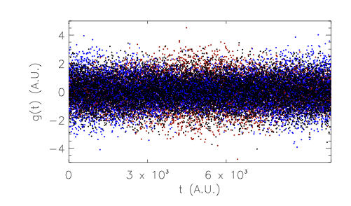
Figure 1: Gaussian random uncorrelated noise (black). The colored points show time series with linear phase correlations among adjacent phases ($\Delta=1$) with $\sigma_{\eta}=1.0$ and $d\phi=0$ (blue) and $d\phi=\pi$ (red).

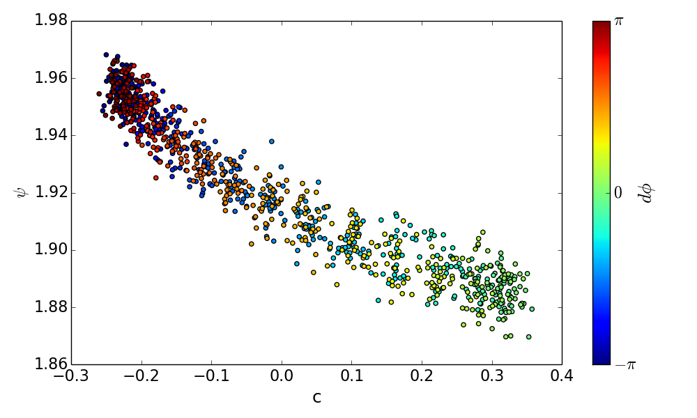
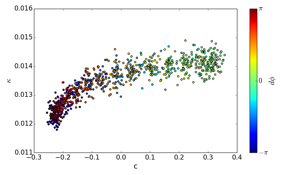
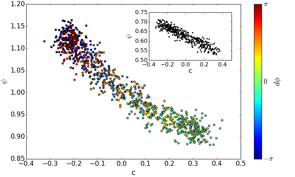
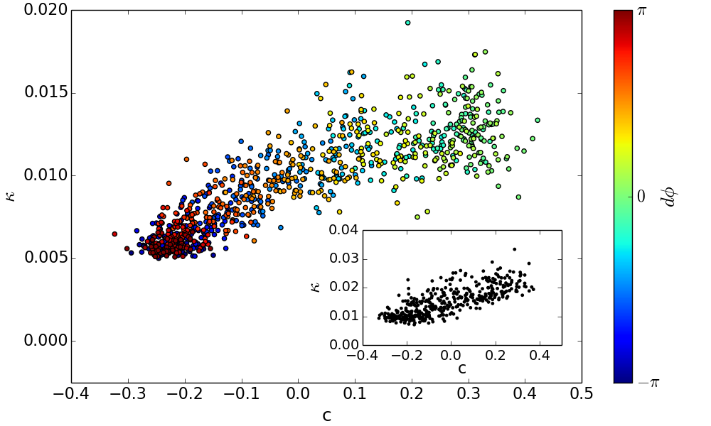
Figure 2: Upper Row: Nonlinear prediction error $\psi$ (upper left) and average connectivity $\kappa$ (upper right) versus phase correlation coefficient $c(\Delta=1)$ for 900 time series with imposed phase correlations derived from Gaussian noise as input time series $g(t)$. Lower row: Same as upper row but with the Mrk 766 X-ray observation as input time series $g(t)$. The data from revolution 999 was binned with a binsize of 50 s leading to a time series with 1540 points. The insets show the corresponding results for 400 IAAFT surrogates.

To allow for a systematic investigation of phase correlations and their corresponding nonlinearities in time series, it is desirable to start with the phases, constrain their correlations in a tunable and reproducible way and study the effects on the nonlinear statistics.
Here, we present a method to generate time series with such tailored nonlinearities by imposing well-defined correlations on the Fourier phases and demonstrate how deviations from linearity can be understood in terms of phase information.
Methods. To address the relationship between phase correlations and measures for nonlinearity we calculate the nonlinear prediction error (NPLE) Sugihara and May (1990) as an example for a dynamical complexity measure with a good overall performance Schreiber and Schmitz (1997) and the average connectivity of (recurrence) networks as an example for a structural complexity measure Donner et al. (2010); Laut et al. (2014). The calculation of both measures relies on the representation of the time series in an artificial phase space, which is obtained using the method of delay coordinates Packard et al. (1980). This is accomplished by using time delayed versions of the observed time series as coordinates for the embedding space. The multivariate vectors in the $d$-dimensional space are expressed by $\vec{g}_{t}=(g_{t},g_{t+\tau},g_{t+2\tau},\ldots,g_{t+(d-1)\tau})\;,$ where $\tau$ is the delay time and $g_{t}$ denotes the value of the (discretized) time series at time step $t$.
The comparison of the predicted behavior of the embedded time series based on the local neighbors with the real trajectory of the system leads to the definition of the NLPE $\psi$ as

$$\psi = \psi(d,\tau,T,N)$$

$$= \frac{1}{(M-T-(d-1)\tau)}\sqrt{\sum_{n=(d-1)\tau}^{M-1-T}[\vec{g}_{t+T}-F(\vec{g}_{t})]^{2}}\;,$$

where $F$ is a locally constant predictor, $M$ is the length of the time series, and $T$ is the lead time. The predictor $F$ is calculated by averaging over future values of the $N=d+1$ nearest neighbors in the delay coordinate representation. We found that $\psi$ remains rather constant for $T>5$, thus a value of $T=5$ was used for this study. The dimension of the embedding space $d$ and the delay time $\tau$ have to be set appropriately. Since the time series of an Active Galactic Nuclei (AGN) being studied in the following consists of less than 1600 data points, we use a low embedding dimension $d=3$. Due to the long correlation time of this time series, we chose a relatively large delay time $\tau=250$ according to the criterion of zero crossing of the autocorrelation function Fraser and Swinney (1986). To allow for a direct comparison, we use the same values $d=3$ and $\tau=250$ for the other time series with imposed phase correlations. The structural complexity of a time series with a limited number of points can be characterized with recurrence networks Marwan et al. (2009). They are based on recurrence plots Eckmann et al. (1987), which describe how often pairs of points of a time series in the embedding space representation come close to each other. Linking such nearby points in a network representation of the data and omitting self-loops leads to the definition of the adjacency matrix $A_{i,j}$ of the recurrence network (Donner et al., 2010)

$$A_{i,j}=\Theta\left(\epsilon-\|\mathbf{g}_{i}-\mathbf{g}_{j}\|\right)-\delta_{i,j},$$ (3)

where the $\{\mathbf{g}_{n}\}$ are the data points in embedding space and $\epsilon$ is an appropriate threshold. $A_{i,j}$ contains the whole information about the network. A common measure for the topological structure of the network is the average connectivity $\kappa$ which is calculated by

$$\kappa=\frac{1}{n(n-1)}\sum_{\nu=0}^{n-1}k_{\nu},$$ (4)

where $k_{\nu}=\sum_{i=0}^{n-1}A_{\nu,i}$ is the degree of node $\nu$. If the attractor of the nonlinear system is reconstructed with appropriate embedding parameters this network measure can be used as a test for nonlinearity. The threshold $\epsilon$ is chosen such that $\kappa=0.01$ for the original time series. The same threshold is then used for the Gaussian time series with imposed phase correlations.
To get a visual impression of correlations among the Fourier phases it is convenient to make use of so-called phase maps Chiang et al. (2002). A phase map is defined as a two-dimensional set of points $G=\{\phi_{k},\phi_{k+\Delta}\}$ where $\phi_{k}$ is the phase of the $k^{th}$ mode of the Fourier transform and $\Delta$ a frequency delay. To quantify the degree of correlation between the phases $\phi$ and $\phi+\Delta$ we calculate the correlation coefficient $c(\Delta)$,

$$c(\Delta)=\frac{\langle\phi(k)\phi(k+\Delta)\rangle}{\sigma_{\phi(k)}\sigma_{\phi(k+\Delta)}}\;.$$ (5)

Note that by using $c(\Delta)$ as correlation measure we restrict ourselves to the simplest way of quantifying correlations among the phases that is only sensitive to linear correlations.

Time series with phase correlations. As outlined in Räth et al. (2011), (I)AAFT surrogates can contain phase correlations leading to statistically significant high or low values of $c(\Delta)$. A closer look at the corresponding phase maps reveals that the (anti-)correlations originated from stripe-like, patterns along the diagonal (i.e. with slope of one) or shifted relative to it. These patters thus indicate that phase pairs are linearly correlated with each other. One can further notice that for the time series stemming from X-ray observations of the AGN Mrk 766 the phase correlations are most pronounced for $\Delta=1$. We reproduce such signatures by imposing correlations in the phase distribution in the following way: The values for the phases $\phi(k)$ are iteratively determined by relating $\phi(k+\Delta)$ with $\phi(k)$ by

$$\phi(k+\Delta)=\phi(k)+d\phi+\eta$$ (6)

with $d\phi$ being a shift constant ranging from $-\pi$ to $\pi$ and $\eta$ describing a (Gaussian) noise term with given standard deviation $\sigma_{\eta}$. In the phase map picture $\eta$ controls the width of the stripes and $d\phi$ defines its position. The iteration is performed over the frequencies $k$, where $k_{s}$ denotes the starting value and $dk$ the step size of the iteration. $\phi(k_{s})$ is drawn from a uniform distribution within the interval $[-\pi,\pi]$. The same is true for $\phi(k)$ if this phase has not been set in a previous iteration step. In our first example we are interested in only correlating adjacent phases. Thus we apply Eq. 6 with $\Delta=1$ to a Gaussian time series with zero mean and standard deviation of one. The step size is chosen to $dk=2$. Thereby every phase is correlated to exactly one other phase for $\Delta=1$, while the phases are not correlated for any frequency delay $\Delta$ greater than one.
Fig. 1 shows how these phase correlations alter the time series. It becomes clearly visible that the correlations of adjacent phases induce fluctuations of the variance. Specifically, one recognizes a time interval where the fluctuations are larger than for the noise and another region where the fluctuations are smaller. Note that the overall mean and standard deviation of the time series are exactly preserved since the power spectrum is kept constant. The shift constant controls the position of the region with higher fluctuations. If $d\phi=0$, this region is located in the middle of the time series and it shifts towards the ends of the time series when $d\phi$ approaches $\pm\pi$. By testing different values of $\Delta$ we further found that the number of regions with high fluctuations is given by the value for $\Delta$. In Fig. 2 we show the nonlinear prediction error $\psi$ and the mean connectivity $\kappa$ as a function of the correlation coefficient $c(\Delta=1)$. The results are displayed for time series with imposed phase correlations (only) for $\Delta=1$ and varying $d\phi$ as derived from Gaussian noise and from the X-ray observation of the AGN Mrk 766. One can see that the shift constant $d\phi$ controls the (anti-)correlations of the phases. More importantly, it becomes obvious that both the nonlinear prediction error and the mean connectivity are highly (anti-)correlated with the phase correlations as measured with $c(\Delta)$. Knowing that $d\phi$ also controls the position of the regions with higher and lower fluctuations, we can now get a much more detailed understanding of how the phase correlations influence the calculation of the NLPE and the average connectivity. The embedding with the delay time of $\tau=250$ in three dimensions leads to a truncation of the last part of the time series. Depending on whether the remaining time series has lower ($d\phi\approx\pm\pi$) or larger ($d\phi\approx 0$) fluctuations, one obtains larger or lower values for the NLPE leading to the observed anti-correlation between psi and c. Similarly, lower fluctuations in the time series lead to a more connected recurrence network and vice versa, correlating $\kappa$ and $c(\Delta)$.

Table 1: Parameters defining the imposed phase correlations

	$\Delta$	$dk$	$k_{s}$	$d\phi$	$\eta$
1. Iteration	1	2	1	3.1415	0.1
2. Iteration	3	3	1	3.0	0.08
3. Iteration	3	3	2	3.0	0.3
4. Iteration	5	5	2	1.4	0.2
5. Iteration	7	7	3	3.1415	0.25
6. Iteration	50	50	2	3.0	0.1

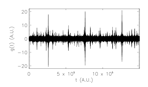
Figure 3: Time series $g(t)$ that is obtained from white Gaussian noise by imposing a set of six different linear phase correlations.

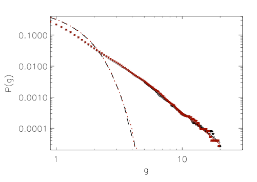
Figure 4: Cumulative probability distribution $P(g)$ of the normalized positive (black) and negative (red) values of $g(t)$. The black dashed and red dotted lines show the respective distributions for the initial white Gaussian noise.

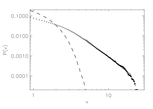
Figure 5: Cumulative probability distribution $P(v)$ of the normalized volatility $v$. The black dashed line shows the respective distributions for the initial white Gaussian noise.

In a second example we extend the formalism to generate nonlinear time series with well-defined nonlinearities by simultaneously imposing linear phase correlations for a set of different frequency delays $\Delta$. This is achieved by iteratively applying Eq. 6 starting with low values of $\Delta$ and then proceeding to higher ones. Iterating over increasing frequency delays $\Delta$ ensures that phase correlations that were imposed in previous iteration steps are at least in parts preserved when new constraints for phase correlations at larger $\Delta$ are added. Table 1 summarizes the parameters for the six iterations used in our example. Fig. 3 shows the time series which is obtained when the six constraints on phase correlations are imposed on white Gaussian noise. One has to note that the time series has no linear correlation as the modulus $|G(k)|$ of the Fourier transform of the original random time series is left untouched. In the time series with phase correlations one can clearly identify a number of time intervals with larger fluctuations whose number, position and strength are controlled by the parameters $\Delta$, $dk$ and $\eta$, respectively. The statistical properties of such a nonlinear time series can thus be tailored in a refined manner. The time series in this example was generated such that it resembles data often observed in economic time series Mantegna and Stanley (2007), where especially data from stock indices show intermittent behavior, i.e. extreme events, patterns of volatility clustering and phase correlations, while the autocorrelation vanishes. The distribution of the fluctuations is further analyzed by calculating the cumulative probability distribution $P(g)$ of the normalized positive and negative values of $g(t)$ (see Fig. 4). We find the expected leptokurtic distribution whose tail can be fitted with a power law $P(g)\sim g^{-\alpha}$ with $\alpha=3.25\pm 0.16$ for the positive tail and $\alpha=3.37\pm 0.47$ for the negative tail in the region $5\leq g\leq 20$. These numbers are in remarkable agreement with those obtained from empirical studies of market indices Gopikrishnan et al. (1999). We further studied the statistical properties of the volatility $v(t)$ as defined as the average of $|g(t)|$ over a time window of length $N$, i.e. $v(t)=1/N\sum_{t^{\prime}=t}^{t+N-1}|g(t^{\prime})|$. Fig. 5 shows the cumulative probability distribution $P(v)$ for $N=5$. As expected we find a distribution with fat tails, which can be fitted by $P(v)\sim v^{-\beta}$ with $\beta=2.93\pm 0.49$ in the region $5\leq v\leq 20$. Again, this is in very good agreement with the scaling properties of the volatility of price fluctuations observed in empirical data Liu et al. (1999).
Finally, we note that analogies between price dynamics of market indices and the velocity differences in three-dimensional fully developed turbulence have been pointed out by several authors (see e.g. Ghashghaie et al. (1996); Mantegna and Stanley (1997)). Consequently, the fat tails in the probability density functions of turbulence data may be also be understood in terms of phase correlations allowing for a better characterization and discrimination of different scenarios of turbulence.

Summary. We have presented a new method to generate time series with well-defined nonlinearities by imposing linear correlations among the Fourier phases. We have shown that the phase correlations between adjacent phases are tightly related with higher order statistics being estimated for the time series. These ”Wiener-Khinchin-like” connections between phase information and higher order statistics are to a large extent independent of the input time series. Furthermore, the scaling of fluctuation and of the volatility of a time series can be understood in terms of a set of linear phase correlations. We expect that further studies with time series and also spatial structures with tailored nonlinearities, for which not only linear but more complex constraints on the Fourier phases are imposed, will shed more light on both the meaning of Fourier phases and the different kinds of nonlinearities as they are observed in nature.

Acknowledgments. This work has made use of observations obtained with XMM-Newton, an ESA science mission with instruments and contributions directly funded by ESA member states and the US (NASA).

References

- Theiler et al. (1992) J. Theiler, S. Eubank, A. Longtin, B. Galdrikian, and J. D. Farmer, Physica D 58, 77 (1992).
- Schreiber and Schmitz (1996) T. Schreiber and A. Schmitz, Phys. Rev. Lett. 77, 635 (1996).
- Keylock (2006) C. J. Keylock, Phys. Rev. E 73, 036707 (2006).
- Keylock (2010) C. J. Keylock, Nonlinear Processes in Geophysics 17, 615 (2010).
- Räth et al. (2012) C. Räth, M. Gliozzi, I. E. Papadakis, and W. Brinkmann, Physical Review Letters 109, 144101 (2012).
- Räth et al. (2009) C. Räth, G. E. Morfill, G. Rossmanith, A. J. Banday, and K. M. Górski, Physical Review Letters 102, 131301 (2009).
- Räth et al. (2011) C. Räth, A. J. Banday, G. Rossmanith, H. Modest, R. Sütterlin, K. M. Górski, J. Delabrouille, and G. E. Morfill, Mon. Not. R. Astron. Soc. 415, 2205 (2011).
- Planck Collaboration et al. (2014) Planck Collaboration, P. A. R. Ade, N. Aghanim, C. Armitage-Caplan, M. Arnaud, M. Ashdown, F. Atrio-Barandela, J. Aumont, C. Baccigalupi, A. J. Banday, et al., Astron. & Astrophys. 571, A23 (2014).
- Modest et al. (2014) H. I. Modest, C. Räth, A. J. Banday, K. M. Górski, and G. E. Morfill, Phys. Rev. D 89, 123004 (2014).
- Sugihara and May (1990) G. Sugihara and R. M. May, Nature (London) 344, 734 (1990).
- Schreiber and Schmitz (1997) T. Schreiber and A. Schmitz, Phys. Rev. E 55, 5443 (1997).
- Donner et al. (2010) R. V. Donner, Y. Zou, J. F. Donges, N. Marwan, and J. Kurths, New Journal of Physics 12, 033025 (2010).
- Laut et al. (2014) I. Laut, C. Räth, L. Wörner, V. Nosenko, S. K. Zhdanov, J. Schablinski, D. Block, H. M. Thomas, and G. E. Morfill, Phys. Rev. E 89, 023104 (2014).
- Packard et al. (1980) N. H. Packard, J. P. Crutchfield, J. D. Farmer, and R. S. Shaw, Physical Review Letters 45, 712 (1980).
- Fraser and Swinney (1986) A. M. Fraser and H. L. Swinney, Phys. Rev. A 33, 1134 (1986).
- Marwan et al. (2009) N. Marwan, J. F. Donges, Y. Zou, R. V. Donner, and J. Kurths, Phys. Lett. A 373, 4246 (2009).
- Eckmann et al. (1987) J.-P. Eckmann, S. Oliffson Kamphorst, and D. Ruelle, EPL (Europhysics Letters) 4, 973 (1987).
- Chiang et al. (2002) L.-Y. Chiang, P. Coles, and P. Naselsky, Mon. Not. R. Astron. Soc. 337, 488 (2002).
- Mantegna and Stanley (2007) R. N. Mantegna and H. E. Stanley, Introduction to Econophysics (Cambridge University Press, Cambridge, UK, 2007).
- Gopikrishnan et al. (1999) P. Gopikrishnan, V. Plerou, L. A. Nunes Amaral, M. Meyer, and H. E. Stanley, Phys. Rev. E 60, 5305 (1999).
- Liu et al. (1999) Y. Liu, P. Gopikrishnan, P. Cizeau, M. Meyer, C.-K. Peng, and H. E. Stanley, Phys. Rev. E 60, 1390 (1999).
- Ghashghaie et al. (1996) S. Ghashghaie, W. Breymann, J. Peinke, P. Talkner, and Y. Dodge, Nature (London) 381, 767 (1996).
- Mantegna and Stanley (1997) R. N. Mantegna and H. E. Stanley, Physica A Statistical Mechanics and its Applications 239, 255 (1997).