HU-EP-15/38

Wilson loops at strong coupling
for curved contours with cusps

Harald Dorn

Institut für Physik und IRIS Adlershof, Humboldt-Universität zu Berlin,
Zum Großen Windkanal 6, D-12489 Berlin, Germany

Abstract

We construct the minimal surface in $AdS$, relevant for the strong coupling behaviour of local supersymmetric Wilson loops in ${\cal N}=4$ SYM for a closed contour formed out of segments of two intersecting circles. Its regularised area is calculated including all divergent parts and the finite renormalised term. Furthermore we prove, that for generic planar curved contours with cusps the cusp anomalous dimensions are functions of the respective cusp angles alone. They do not depend on other local data of the cusps.

1 Introduction

The renormalisation properties of Wilson loops in perturbative gauge theories are well understood for a long time [1, 2, 3, 4, 5]. With smooth closed contours there appears an exponential of a linear divergence proportional to the length of the contour. Besides removing this factor and the renormalisation of the coupling constant, no further renormalisation is needed to get finite results. This changes if the contour has cusps or self-intersections, where additional logarithmic divergences show up. The corresponding cusp anomalous dimension has been calculated for QCD in one [1], two [6] and three loop order [7].

In ${\cal N}=4$ SYM the situation improves. At first the theory is conformally invariant and the coupling needs no renormalisation, and for local supersymmetric loops the linear divergences cancel [8]. The logarithmic cusp divergences are still present and of great interest for a lot of applications, a recent calculation up to the four loop order in planar ${\cal N}=4$ SYM one finds in [9].

But even more important, with the $AdS$/CFT correspondence one has a handle to the strong coupling behaviour. At strong ’t Hooft coupling $\lambda$, the locally supersymmetric Wilson loop for a closed contour ${\cal C}$ is in leading order given by [10, 11]

$$W({\cal C})~{}=~{}\mbox{exp}\Big{(}-\frac{\sqrt{\lambda}}{2\pi}~{}A({\cal C})\Big{)}~{}.$$ (1)

$A({\cal C})$ is the area of a minimal surface extending into the bulk of $AdS_{5}$ and approaching its boundary along the contour ${\cal C}$. The construction uses Poincaré coordinates

$$ds^{2}~{}=~{}\frac{1}{r^{2}}\big{(}dx^{\mu}dx_{\mu}~{}+~{}dr^{2}\big{)}~{},$$ (2)

where the conformal boundary is at $r=0$. The UV divergences of the gauge theory reappear as divergences due to the blow up of the metric near $r=0$. The standard procedure to define a regularised area $A_{\epsilon}$ is based on cutting off that part of the surface on which $r<\epsilon$.

For the interpolation between weak and strong coupling, integrability techniques have been used in [12] to derive a set of equations for the cusp anomalous dimension.

Solving the minimal surface condition (equation of motion, if seen as string surface) near the boundary of $AdS$, one gets for space-like contours [13, 14]

$$x^{\mu}(\sigma,r)~{}=~{}x^{\mu}(\sigma,0)~{}+~{}\frac{1}{2}\frac{d^{2}}{d\sigma^{2}}x^{\mu}(\sigma,0)~{}r^{2}~{}+~{}{\cal O}(r^{3})~{},$$ (3)

where $\sigma$ together with the fifth $AdS$ coordinate $r$ parameterises the surface and is the length parameter on the boundary curve $x^{\mu}(\sigma,0)$. The absence of a term linear in $r$ in eq.(3) ensures that for smooth boundary curves with their bounded curvature one gets ($l$ length of the Wilson loop contour)

$$A_{\epsilon}~{}=~{}\frac{l}{\epsilon}~{}+~{}A_{\mbox{\tiny ren}}~{}+~{}{\cal O}(\epsilon)~{}.$$ (4)

The invariance of $A_{\mbox{\tiny ren}}$ under conformal rescalings of the metric on the boundary of $AdS$ has been proven in [13]. The equivalent issue of keeping the metric fixed, but performing an active conformal mapping of the boundary points has been discussed on the level of infinitesimal transformations in [15]. A direct proof for finite transformations can be given by using (3) and applying Stokes theorem on that part of the original surface bounded by the line $r=\epsilon$ and the preimage of the line which is at the same value of $r$ on the mapped surface.

In the presence of cusps the expansion in (3) with uniformly bounded coefficients breaks down. This is the reason for the appearance of logarithmic divergences in $A_{\epsilon}$ for $\epsilon\rightarrow 0$. For a generic smooth contour with $n$ cusp one commonly expects

$$A_{\epsilon}~{}=~{}\frac{l}{\epsilon}~{}+~{}\sum_{i=1}^{n}~{}\Gamma_{\mbox{\tiny cusp}}(\theta_{i})~{}\mbox{log}~{}\epsilon~{}+~{}A_{\mbox{\tiny ren}}+~{}{\cal O}(\epsilon)~{}.$$ (5)

Now we are ready to pose the question treated in this paper. All calculations of the coefficient in the logarithmic divergence have been performed for a cusp with straight legs [8, 19], and it is commonly believed that the above structure, with the same $\Gamma_{\mbox{\tiny cusp}}$ depending only on the cusp angles $\theta_{i}$, is true also for cusps with curved legs. We want to prove that this belief is justified indeed. Of course, it is clear that $\Gamma_{\mbox{\tiny cusp}}$ can depend on dimensionless local data only. But for generic cusps there are available, besides the angles, e.g. the quotients of the right and left limits of the curvature.

In the case of the field theoretic small coupling expansion the use of the simplification achieved by working with straight legs is easier to justify. In comparison to the smooth case, these divergences are due to the change generated by the cusp into the projection of four-dimensional distances $(x-y)^{2}$ onto the one-dimensional contour parameter space.

The paper is organised as follows. In section 2 we calculate $A_{\epsilon}$ for contours formed out of segments of two intersecting circles with arbitrary radii, including all divergent terms as well as $A_{\mbox{\tiny ren}}$. The result for this example will fit into the structure (5).

Section 3 is devoted to generic contours in an Euclidean plane. A suitable surface parameterisation for generic cusps with curved legs is developed as some kind of perturbation of that used in the case of straight legs in [8]. Then on its basis a general proof will be given.

Several technical details are collected in six appendices.

2 Contour with two cusps, formed by segments of two circles

Two straight half-lines, starting on the $x_{1}$-axis at $x_{1}=q>0$ with angles $\gamma_{1}<\gamma_{2}$, form a cusp with angle

$$\theta=\gamma_{2}-\gamma_{1}.$$ (6)

The corresponding minimal surface is given by [8]

$$x_{1}~{}=~{}q~{}+~{}\rho~{}\mbox{cos}(\varphi+\gamma_{1})~{},~{}~{}~{}~{}~{}~{}~{}x_{2}~{}=~{}\rho~{}\mbox{sin}(\varphi+\gamma_{1})~{},~{}~{}~{}~{}~{}~{}~{}r~{}=~{}\frac{\rho}{f(\varphi)}~{},$$ (7)

with $0\leq\rho<\infty~{},~{}~{}~{}0\leq\varphi\leq\theta$. The essential properties of this solution are summarised in appendix B, in particular $f(\varphi)$ is defined implicitely by eqs. (77),(78).

The map

$$x_{\mu}~{}\mapsto~{}y_{\mu}~{}=~{}\frac{x_{\mu}}{x^{2}+r^{2}}~{},~{}~{}~{}~{}~{}r~{}\mapsto~{}z~{}=~{}\frac{r}{x^{2}+r^{2}}~{}$$ (8)

is an isometry inside $AdS$ and acts as a conformal transformation on the boundary (inversion at the unit circle). It maps the two half-lines discussed above to segments of two circles forming a closed contour with two cusps, both with angle $\theta$ . For some details see appendix A.

Due to the bulk isometry property of (8), the minimal surface related to this closed contour is then given by

$$y_{1} = \frac{\rho~{}\mbox{cos}(\varphi+\gamma_{1})~{}+~{}q}{\rho^{2}+q^{2}+2q\rho~{}\mbox{cos}(\varphi+\gamma_{1})+(\rho/f(\varphi))^{2}}~{},$$

$$y_{2} = \frac{\rho~{}\mbox{sin}(\varphi+\gamma_{1})}{\rho^{2}+q^{2}+2q\rho~{}\mbox{cos}(\varphi+\gamma_{1})+(\rho/f(\varphi))^{2}}~{},$$

$$z = \frac{\rho/f}{\rho^{2}+q^{2}+2q\rho~{}\mbox{cos}(\varphi+\gamma_{1})+(\rho/f(\varphi))^{2}}~{}.$$ (9)

For all surfaces we follow the standard definition of the regularised area, i.e. cutting off that part of the surface whose Poincaré $r$-coordinate (see (2)) is smaller than $\epsilon$. Since we denoted this coordinate for our surface generated by the map (8) with the letter $z$, we have to calculate

$$A_{\epsilon}~{}=~{}\int_{z>\epsilon}\sqrt{h}~{}d\rho d\varphi~{},$$ (10)

where $h$ is the determinant of the induced metric on the surface (9). There is an alternative way to get the same quantity: calculate the area of the preimage of the cut surface on the original (7). Then for $h$ one has to take the simple form as in (75) of appendix B and the integration region for $\rho$ at fixed allowed $\varphi$ is given by

$$\rho_{-}<\rho<\rho_{+}~{},$$ (11)

with

$$\rho_{\pm}=\frac{1-2\epsilon qf(\varphi)\mbox{cos}(\varphi+\gamma_{1})\pm\sqrt{1-4\epsilon qf\mbox{cos}(\varphi+\gamma_{1})-4\epsilon^{2}q^{2}f^{2}\mbox{sin}^{2}(\varphi+\gamma_{1})-4\epsilon^{2}q^{2}}}{2\epsilon(f+1/f)}$$

denoting the two solutions of the equation $z=\epsilon$. The square root in the above formula has to be real. This gives implicit bounds for $\varphi$ via

$$f_{0}~{}<~{}f(\varphi)~{}<~{}f_{\epsilon}~{}.$$ (12)

To characterise $f_{\epsilon}$, one has to handle the fact that the relation between $\varphi$ and $f$ is not one to one. Instead we have $f(\varphi)=f(\theta-\varphi)$, and in $\varphi\in(0,\theta/2)$ the function $\varphi(f)$ is given by formula (78) of appendix B. Therefore, we split the regularised area $A_{\epsilon}$ into two pieces, one originating from $\varphi\in(0,\theta/2)$ and the other from $\varphi\in(\theta/2,\theta)$

$$A_{\epsilon}~{}=~{}A_{\epsilon}^{(1)}~{}+~{}A_{\epsilon}^{(2)}~{}.$$ (13)

Having in mind $\varphi+\gamma_{1}=\gamma_{2}-(\theta-\varphi)$, we define $f_{\epsilon}^{(j)}$ ($j=1,2$) by

$$f_{\epsilon}^{(j)}~{}=~{}\frac{\sqrt{1-4\epsilon^{2}q^{2}\mbox{sin}^{2}\big{(}\gamma_{j}\pm\varphi(f_{\epsilon}^{(j)})\big{)}~{}}-\mbox{cos}\big{(}\gamma_{j}\pm\varphi(f_{\epsilon}^{(j)})\big{)}}{2\epsilon~{}q~{}\mbox{sin}^{2}\big{(}\gamma_{j}\pm\varphi(f_{\epsilon}^{(j)})\big{)}}~{}.$$ (14)

Estimating this implicit definition for $\epsilon\rightarrow 0$, which is correlated with $f_{\epsilon}^{(j)}\rightarrow\infty$ and via (81) with $\varphi(f_{\epsilon}^{(j)})\rightarrow 0$ this simplifies to

$$f_{\epsilon}^{(j)}~{}=~{}\frac{T_{j}}{\epsilon}~{}-~{}q~{}+~{}{\cal O}(\epsilon)~{},~{}~{}~{}~{}~{}\mbox{with}~{}~{}~{}~{}~{}T_{j}~{}=~{}\frac{1-\mbox{cos}\gamma_{j}}{2q~{}\mbox{sin}^{2}\gamma_{j}}~{}.$$ (15)

After substituting the integration variables $\varphi$ or $\theta-\varphi$, respectively, via (78) of appendix B by $f$, we get for $j=1,2$

$$A_{\epsilon}^{(j)} = \int_{f_{0}}^{f_{\epsilon}^{(j)}}df\int_{\rho_{-}(f)}^{\rho_{+}(f)}\frac{d\rho}{\rho}\sqrt{\frac{f^{4}+f^{2}}{f^{4}+f^{2}-E^{2}}}$$ (16)

$$= \int_{f_{0}}^{f_{\epsilon}^{(j)}}df~{}\sqrt{\frac{f^{4}+f^{2}}{f^{4}+f^{2}-E^{2}}}~{}\Big{(}2~{}\mbox{log}\frac{\rho_{+}^{(j)}(f)}{q}~{}+~{}\mbox{log}\frac{1+f^{2}}{f^{2}}\Big{)}~{},$$

where we used that (11) implies $\rho_{+}^{(j)}\rho_{-}^{(j)}=\frac{q^{2}f^{2}}{1+f^{2}}$. Here $\rho_{\pm}^{(1)}$ is given by the r.h.s of (11) and $\rho_{\pm}^{(2)}$ after the replacement of $\gamma_{1}+\varphi(f)$ by $\gamma_{2}-\varphi(f)$.

Let us now separate $A_{\epsilon}^{(j)}$ into two additive pieces, where only the first one contains the function $\varphi(f)$

$$A_{\epsilon}^{(j)} = A_{\epsilon}^{(j,1)}~{}+~{}A_{\epsilon}^{(j,2)}~{},$$ (17)

$$A_{\epsilon}^{(j,1)} = 2~{}\int_{f_{0}}^{f_{\epsilon}^{(j)}}df~{}\sqrt{\frac{f^{4}+f^{2}}{f^{4}+f^{2}-E^{2}}}~{}\mbox{log}N_{\epsilon}^{(j)}(q,f)~{},$$ (18)

$$A_{\epsilon}^{(j,2)} = -~{}\int_{f_{0}}^{f_{\epsilon}^{(j)}}df~{}\sqrt{\frac{f^{4}+f^{2}}{f^{4}+f^{2}-E^{2}}}~{}\big{(}2\mbox{log}(2q\epsilon)~{}+~{}\mbox{log}(1+f^{2})\big{)}~{}.$$ (19)

$N_{\epsilon}^{(j)}(q,f_{0},f)$ is the nominator in (11), i.e.

$$N_{\epsilon}^{(j)}(q,f) = 1-2\epsilon qf\mbox{cos}(\varphi(f)\pm\gamma_{j})$$

$$+~{}\sqrt{1-4\epsilon qf\mbox{cos}(\varphi\pm\gamma_{j})-4\epsilon^{2}q^{2}f^{2}\mbox{sin}^{2}(\varphi\pm\gamma_{j})-4\epsilon^{2}q^{2}}~{}.$$

The straightforward evaluation of $A_{\epsilon}^{(j,2)}$ gives, using (15) and (86),

$$A_{\epsilon}^{(j,2)} = \Gamma_{\mbox{\tiny cusp}}(\theta)~{}\mbox{log}(2q\epsilon)~{}+~{}\frac{1-\mbox{cos}\gamma_{j}}{\epsilon~{}q\mbox{sin}^{2}\gamma_{j}}~{}\Big{(}1-\mbox{log}(\frac{1-\mbox{cos}\gamma_{j}}{\mbox{sin}^{2}\gamma_{j}})\Big{)}$$ (21)

$$-\int_{f_{0}}^{\infty}df~{}\left(\sqrt{\frac{f^{4}+f^{2}}{f^{4}+f^{2}-E^{2}}}-1\right)~{}\mbox{log}(1+f^{2})~{}+~{}2q~{}\mbox{log}(2qT_{j})$$

$$~{}+~{}f_{0}~{}\mbox{log}(1+f_{0}^{2})~{}+~{}2~{}\mbox{arctan}f_{0}-2f_{0}-\pi~{}+~{}{\cal O}(\epsilon~{}\mbox{log}\epsilon)~{}.$$

The bit more involved evaluation of $A_{\epsilon}^{(j,1)}$ is discussed in some detail in appendix C, with the result given in (97). Making use of the definition of $\Gamma_{\mbox{\tiny cusp}}(\theta)$ in eq.(86) of appendix B it appears as

$$A_{\epsilon}^{(j,1)} = \frac{2}{q\epsilon}~{}\left(\frac{\gamma_{j}}{2~{}\mbox{sin}\gamma_{j}}-\frac{1+\mbox{log}(1+\mbox{cos}\gamma_{j})}{4~{}\mbox{cos}^{2}\frac{\gamma_{j}}{2}}\right)$$ (22)

$$~{}-~{}\Gamma_{\mbox{\tiny cusp}}(\theta)~{}\mbox{log}2~{}-~{}2q~{}\mbox{log}\Big{(}\frac{1-\mbox{cos}\gamma_{j}}{\mbox{sin}^{2}\gamma_{j}}\Big{)}~{}+~{}\mbox{{\tiny\cal O}}(1)~{},$$

and then the sum (17) is

$$A_{\epsilon}^{(j)} = \Gamma_{\mbox{\tiny cusp}}(\theta)~{}\mbox{log}(q\epsilon)~{}+~{}\frac{\gamma_{j}}{\epsilon~{}q~{}\mbox{sin}\gamma_{j}}~{}+~{}f_{0}~{}\mbox{log}(1+f_{0}^{2})~{}+~{}2~{}\mbox{arctan}f_{0}-2f_{0}-\pi$$ (23)

$$-~{}\int_{f_{0}}^{\infty}df~{}\left(\sqrt{\frac{f^{4}+f^{2}}{f^{4}+f^{2}-E^{2}}}-1\right)~{}\mbox{log}(1+f^{2})~{}~{}+~{}\mbox{{\tiny\cal O}}(1)~{}.$$

To perform the ambiguous separation into a divergent and finite part we have to introduce an RG-scale $\mu$. Then we get for the total area (13)

$$A_{\epsilon}~{}=~{}2\Gamma_{\mbox{\tiny cusp}}(\theta)~{}\mbox{log}(\mu\epsilon)~{}+~{}\frac{l}{\epsilon}~{}+~{}{\cal O}(1)~{}.$$ (24)

Here we have made use of appendix A, eq.(72) to confirm also for this explicit example the generic property, that the factor for the linear divergence is given by the length of the contour.

The renormalised area is ($Q=1/q$ distance between the cusps, see (66))

$$A_{\mbox{\tiny ren}} = -2\Gamma_{\mbox{\tiny cusp}}(\theta)~{}\mbox{log}\big{(}\mu Q\big{)}~{}+~{}2f_{0}~{}\mbox{log}(1+f_{0}^{2})~{}+~{}4~{}\mbox{arctan}f_{0}-4f_{0}-2\pi$$ (25)

$$-~{}2~{}\int_{f_{0}}^{\infty}df~{}\left(\sqrt{\frac{f^{4}+f^{2}}{f^{4}+f^{2}-f_{0}^{4}-f_{0}^{2}}}-1\right)~{}\mbox{log}(1+f^{2})~{}.$$

It has a remarkable structure. There is a conformally invariant contribution depending only on the cusp angle $\theta$, via $f_{0}(\theta)$ given in (79). Dependence on other data of our contour appear only via the first term, whose presence is enforced by the RG-ambiguity and which breaks conformal invariance. There this dependence comes via the distance between the two cusps $Q$, which by (66) and (69) is given as a function of the radii of the two circles and the distance of their centers.

Since the linear divergence is $l/\epsilon$, perhaps the most natural choice for the RG scheme is minimal subtraction with respect to $l/\epsilon$. This corresponds to $\mu=1/l$. Then $A_{\mbox{\tiny ren}}$ depends on the cusp angle $\theta$ and the ratio $Q/l$.

Closing this section, let us consider the limit in which our contour becomes a circle. Then one has $\theta=\pi$, i.e $f_{0}=0$ and $Q=2R$. Since $\Gamma_{\mbox{\tiny cusp}}(\pi)=0$, this gives

$$A_{\mbox{\tiny ren}}^{\mbox{\tiny circle}}~{}=~{}-2\pi~{},$$ (26)

in agreement with the literature [8, 17, 18].

3 Cusp anomalous dimension in the generic case

Let us consider a closed contour in the $(x_{1},x_{2})$-plane with a cusp, located at the origin, but smooth otherwise. At first we divide the related minimal surface in two parts, depending on whether $\rho=\sqrt{x_{1}^{2}+x_{2}^{2}}$ is smaller or larger then a certain value. This $\rho_{0}$ should be small, but kept fixed for $\epsilon\rightarrow 0$. The corresponding regularised area is then given by

$$A_{\epsilon}~{}=~{}A_{\epsilon}^{\tiny\mbox{cusp}}(\rho_{0})~{}+~{}A_{\epsilon}^{\tiny\mbox{smooth}}(\rho_{0})~{}.$$ (27)

Due to the general result for smooth contours we know already

$$A_{\epsilon}^{\tiny\mbox{smooth}}(\rho_{0})~{}=~{}\frac{l-l_{\rho_{0}}}{\epsilon}~{}+~{}{\cal O}(1)~{},$$ (28)

where $l$ is the length of the total contour and $l_{\rho_{0}}$ that of the cusp piece.

Let now the two curved legs of the cusp be parameterised in the vicinity of the origin by

$$x^{(j)}_{1}~{}=~{}\rho~{}\mbox{cos}\big{(}\phi^{(j)}(\rho)\big{)}~{},~{}~{}~{}~{}x^{(j)}_{2}~{}=~{}\rho~{}\mbox{sin}\big{(}\phi^{(j)}(\rho)\big{)}~{},~{}~{}~{}~{}j=1,2~{}.$$ (29)

The cusp angle $\theta$ is then given by

$$\theta~{}=~{}\phi_{2}(0)~{}-~{}\phi_{1}(0)~{},$$ (30)

and the $\rho\rightarrow 0$ limits of the curvatures of both legs are

$$k_{j}~{}=~{}2c_{j}~{}=~{}2~{}\frac{d\phi^{(j)}}{d\rho}\Big{|}_{\rho=0}~{}.$$ (31)

The length $l_{\rho_{0}}$ turns out to be

$$l_{\rho_{0}}~{}=~{}2\rho_{0}~{}+~{}\frac{1}{6}(c_{1}^{2}+c_{2}^{2})\rho_{0}^{3}~{}+~{}{\cal O}(\rho_{0}^{4})~{}.$$ (32)

For the evaluation of $A_{\epsilon}^{\tiny\mbox{cusp}}(\rho_{0})$ we want to work with coordinates $\rho~{},\varphi$ for the $(x_{1},x_{2})$-plane, adapted in a manner that still $\rho^{2}=x_{1}^{2}+x_{2}^{2}$, but that the lines of constant $\varphi=0$ and $\varphi=\theta$, respectively, agree with the curved legs forming the cusp. The first requirement is realised by the structure

$$x_{1}~{}=~{}\rho~{}u(\rho,\varphi)~{},~{}~{}~{}~{}x_{2}~{}=~{}\rho~{}\sqrt{1-u^{2}}~{},$$ (33)

and the second one means in addition

$$u(\rho,0)~{}=~{}\mbox{cos}\big{(}\phi^{(1)}(\rho)\big{)}~{},~{}~{}~{}u(\rho,\theta)~{}=~{}\mbox{cos}\big{(}\phi^{(2)}(\rho)\big{)}~{}.$$ (34)

The additional $AdS$-coordinate $r$ we parameterise by

$$r~{}=~{}\rho~{}F(\rho,\varphi)~{},$$ (35)

with the boundary condition

$$F(\rho,0)~{}=~{}F(\rho,\theta)~{}=~{}0~{}.$$ (36)

Then the regularised area of the cusp piece is given by

$$A_{\epsilon}^{\tiny\mbox{cusp}}(\rho_{0})~{}=~{}\int_{r>\epsilon,~{}\rho<\rho_{0}}L(\rho,\varphi)~{}d\rho d\varphi~{},$$ (37)

with

$$L(\rho,\varphi)=\sqrt{\frac{F^{\prime 2}\big{(}1-u^{2}+\rho^{2}\dot{u}^{2}\big{)}+\big{(}1+(F+\rho\dot{F})^{2}\big{)}u^{\prime 2}-2\rho F^{\prime}\big{(}F+\rho\dot{F}\big{)}\dot{u}u^{\prime}}{\rho^{2}F^{4}(1-u^{2})}}~{}.$$ (38)

We will look for perturbative solutions of the related equation of motion in the form

$$F(\rho,\varphi)~{}=~{}F_{1}(\varphi)~{}+~{}\rho~{}F_{2}(\varphi)~{}+~{}\dots~{},$$ (39)

with the boundary conditions

$$F_{n}(0)~{}=~{}F_{n}(\theta)~{}=~{}0~{},~{}~{}~{}~{}n=1,2,\dots~{}~{}.$$ (40)

As a more concrete form for $u$ we now take

$$u(\rho,\varphi)~{}=~{}\mbox{cos}\left(\frac{\rho~{}s(\varphi)+\varphi}{\theta}~{}\big{(}\phi_{2}(\rho)-\phi_{1}(\rho)\big{)}~{}+~{}\phi_{1}(\rho)\right)~{},$$ (41)

where the function $s(\varphi)$ has to be chosen with the behaviour

$$s(\varphi) = a_{1}~{}\varphi^{2/3}~{}+~{}\dots~{}~{},~{}~{}~{}~{}~{}~{}~{}~{}~{}~{}\varphi\rightarrow 0~{},$$

$$s(\varphi) = a_{2}~{}(\theta-\varphi)^{2/3}~{}+~{}\dots~{}~{},~{}~{}~{}\varphi\rightarrow\theta~{}.$$ (42)

The $a_{j}$ are constants to be fixed later.

Let us stop for a moment in order to comment on the need for this peculiar $s(\varphi)$. Naively one would of course start with $s(\varphi)$ put to zero in (41). But then, as we will see below, the boundary condition (40) for $F_{2}$ cannot be fulfilled. For more intuitive arguments for this ansatz, beyond this a posteriori justification, see appendix D. There one also finds in fig.3 a visualisation of the difference of coordinates with and without $s(\varphi)$.

The variational derivative of (38) with respect to $F$ appears as a quotient. We take as the equation of motion the vanishing of the nominator, insert (41) and expand the result with respect to $\rho$. Then the condition, that in this expansion the coefficients of the leading and nextleading term vanish, leads to

$$2(F_{1}^{\prime})^{2}+(1+F_{1}^{2})(2+F_{1}^{2}+F_{1}F_{1}^{\prime\prime})~{}=~{}0$$ (43)

and

$$F_{2}^{\prime\prime}(\varphi)+G_{1}(\varphi)F_{2}^{\prime}(\varphi)+G(\varphi)F_{2}(\varphi)+M(\varphi)~{}=~{}0~{},$$ (44)

in which

$$M(\varphi) = \frac{-1}{\theta(F_{1}+F_{1}^{3})}~{}\Big{\{}~{}\theta(F_{1}+F_{1}^{3})F_{1}^{\prime}~{}s^{\prime\prime}(\varphi)$$

$$~{}~{}~{}~{}~{}+\big{(}c_{1}(\theta-\varphi)+c_{2}\varphi+\theta s(\varphi)\big{)}\big{(}2F_{1}(F_{1}^{\prime})^{3}+F_{1}F_{1}^{\prime}(7+3F_{1}^{2})\big{)}$$

$$~{}~{}~{}~{}~{}~{}~{}+\big{(}c_{1}-c_{2}-\theta s^{\prime}(\varphi)\big{)}(1+F_{1}^{2})\big{(}6+3F_{1}^{2}+2(F_{1}^{\prime})^{2}+F_{1}F_{1}^{\prime\prime}\big{)}\Big{\}}~{},$$

$$G(\varphi) = \frac{13F_{1}+7F_{1}^{3}+2F_{1}(F_{1}^{\prime})^{2}+(1+5F_{1}^{2})F_{1}^{\prime\prime}}{F_{1}+F_{1}^{3}}~{},$$ (46)

$$G_{1}(\varphi) = \frac{2(2-F_{1}^{2})~{}F_{1}^{\prime}}{F_{1}+F_{1}^{3}}~{}.$$ (47)

As expected, the leading order equation (43) depends on $F_{1}$ only. Moreover, it equals that for the full $F$ in the case with straight legs, see (84). Therefore we know from appendix B $F_{1}(\varphi)=F_{1}(\theta-\varphi)$ and in particular from eq.(82)

$$F_{1}(\varphi)~{}=~{}a\varphi^{1/3}~{}+~{}\frac{a^{3}}{5}\varphi~{}+~{}{\cal O}(\varphi^{5/3})~{},~{}~{}~{}~{}a=(3/E)^{1/3}~{}.$$ (48)

Since our concern are divergent contributions to the regularised area

$$A_{\epsilon}~{}=~{}\int_{\rho F(\rho,\varphi)>\epsilon}L(\rho,\varphi)d\rho d\varphi$$ (49)

for $\epsilon\rightarrow 0$, we also have to control the behaviour of $F_{2}$ near the $AdS$ boundary. We will do this for $\varphi\rightarrow 0$, the case $\varphi\rightarrow\theta$ looks similarly. From (42) and (48) we get for $\varphi\rightarrow 0$

$$M(\varphi) = \frac{2(aa_{1}-a^{3}c_{1})}{27\varphi^{2}}~{}+~{}\frac{8(2a^{3}a_{1}-a^{5}c_{1})}{135\varphi^{4/3}}~{}+~{}{\cal O}(1/\varphi)~{},$$ (50)

$$G(\varphi) = -\frac{2}{9\varphi^{2}}~{}-~{}\frac{28a^{2}}{45\varphi^{4/3}}~{}+~{}{\cal O}(\varphi^{-2/3})~{},$$ (51)

$$G_{1}(\varphi) = \frac{4}{3\varphi}~{}-~{}\frac{22a^{2}}{15\varphi^{1/3}}~{}+~{}{\cal O}(\varphi^{1/3})~{}.$$ (52)

Due to this type of singular behaviour of its coefficient functions, the differential equation for $F_{2}(\varphi)$ is singular at $\varphi=0$. Since $\varphi^{2}M~{},~{}\varphi^{2}G$ and $\varphi G_{1}$ are analytic in $x=\varphi^{1/3}$, we have a regular singular point, and $F_{2}$ can be represented as a Frobenius series in $x$. Inserting the leading plus nextleading terms for $G$, $G_{1}$ and $M$ from (50)-(52) into (44) one gets ($B_{1},B_{2}$ integration constants)

$$F_{2}(\varphi) = \frac{1}{3}(aa_{1}-a^{3}c_{1})-\frac{(4a^{3}a_{1}-2a^{5}c_{1})}{15}~{}\varphi^{2/3}+{\cal O}(\varphi)$$

$$~{}~{}~{}~{}~{}~{}~{}~{}~{}+B_{1}\big{(}\varphi^{-2/3}+\frac{8}{5}a^{2}+{\cal O}(\varphi^{2/3})\big{)}+B_{2}\big{(}\varphi^{1/3}+a^{2}\varphi+{\cal O}(\varphi^{5/3})\big{)}~{}.$$

This expression contains three so far unfixed parameters of quite different origin. $a_{1}$ specifies the choice of the coordinate system and $B_{1}$ and $B_{2}$ are the free parameters in the general solution of the differential equation. Now the boundary condition $F_{2}(0)=0$ requires first of all $B_{1}=0$ in order to prevent a divergence. But then there is still the first term on the r.h.s. of (3) obstructing the boundary condition. It vanishes only for the choice

$$a_{1}~{}=~{}a^{2}c_{1}~{}.$$ (54)

As announced above, we see that without $s(\varphi)$ in (41) the boundary condition for $F_{2}$ cannot be fulfilled, if the corresponding leg of the cusp is curved . Fixing $B_{2}$ (and $a_{2}$ in (42)) is a matter of the boundary condition on the second leg of the cusp.

To analyse the regularised area (49), we expand $L(\rho,\varphi)$ with respect to $\rho$

$$L(\rho,\varphi)~{}=~{}\frac{1}{\rho}~{}L_{1}(\varphi)~{}+~{}L_{2}(\varphi)~{}+~{}{\cal O}(\rho)~{}.$$ (55)

Then we get with (38),(39),(41)

$$L_{1}(\varphi)~{}=~{}\frac{\sqrt{1+F_{1}^{2}+(F_{1}^{\prime})^{2}}}{F_{1}^{2}}~{},$$ (56)

$$L_{2}(\varphi) = \frac{1}{\theta~{}F_{1}^{3}\sqrt{1+F_{1}^{2}+(F_{1}^{\prime})^{2}}}~{}\Big{\{}\big{(}c_{2}-c_{1}+\theta s^{\prime}(\varphi)\big{)}\big{(}F_{1}+F_{1}^{3}\big{)}$$

$$-\big{(}c_{1}(\theta-\varphi)+c_{2}\varphi+\theta s(\varphi)\big{)}F_{1}^{2}F_{1}^{\prime}-2\theta\big{(}1+(F_{1}^{\prime})^{2}\big{)}F_{2}+\theta F_{1}F_{1}^{\prime}F_{2}^{\prime}\Big{\}}~{}.$$

Due to the asymptotics (48) this means for $\varphi\rightarrow 0$

$$L_{1}(\varphi)~{}=~{}\frac{1}{3a\varphi^{4/3}}~{}+~{}\frac{a}{15\varphi^{2/3}}~{}+~{}{\cal O}(1)~{},$$ (58)

and via (48),(3) and (54)

$$L_{2}(\varphi)~{}=~{}-B_{2}\Big{(}\frac{1}{3a^{2}\varphi^{4/3}}~{}+{\cal O}(\frac{1}{\varphi^{2/3}})\Big{)}~{}+~{}\frac{c_{1}}{a\varphi^{1/3}}~{}+~{}{\cal O}(1)~{}.$$ (59)

If $B_{2}\neq 0$, the integral of $L_{2}(\varphi)$ is still divergent. The further analysis would be simpler if we could put $B_{2}=0$. But, as mentioned already and elaborated in more detail in appendix E, fixing $B_{2}$ is a matter of the boundary condition on the second leg ($\varphi\rightarrow\theta$), and for generic situations we have to live with $B_{2}\neq 0$.

The divergences in (37) arise from the neighbourhood of $\rho=0$, $\varphi=0$ and $\varphi=\theta$. To keep them under control with the above estimates, we write

$$A_{\epsilon}^{\tiny\mbox{cusp}}(\rho_{0})~{}=~{}A_{\epsilon}^{\tiny\mbox{c},0}(\rho_{0})~{}+~{}A_{\epsilon}^{\tiny\mbox{c},\theta}(\rho_{0})$$ (60)

and understand the first term on the r.h.s with the $\varphi$-integration over the interval $(0,\theta/2$) and the second one over $(\theta/2,\theta)$. Then one has for the second order contribution to $A_{\epsilon}^{\tiny\mbox{c},0}(\rho_{0})$

$$~{}A_{\epsilon,2}^{\tiny\mbox{c},0}(\rho_{0}) = \int_{\rho<\rho_{0},~{}~{}\rho F_{1}+\rho^{2}F_{2}+{\cal O}(\rho^{3})>\epsilon}~{}L_{2}(\varphi)~{}d\rho d\varphi$$ (61)

$$= -\frac{B_{2}}{3a^{2}}\int_{\rho_{min}(\epsilon)}^{\rho_{0}}d\rho\int^{\theta/2}_{(a\rho+B_{2}\rho^{2})\varphi^{1/3}+{\cal O}(\rho^{3})=\epsilon}~{}d\varphi~{}\varphi^{-4/3}~{}+~{}{\cal O}(1)$$

$$= -\frac{1}{\epsilon}~{}\Big{(}\frac{B_{2}}{2a}~{}\rho_{0}^{2}+\frac{B_{2}^{2}}{3a^{2}}~{}\rho_{0}^{3}+{\cal O}(\rho_{0}^{4})\Big{)}~{}+~{}{\cal O}(1)~{}.$$

Use has been made of (59) and $\rho_{min}={\cal O}(\epsilon)$.

The integrand of the leading order contribution $A_{\epsilon,1}^{\tiny\mbox{c},0}(\rho_{0})$ is the same as for the case with a cusp between straight legs. However, the integration region depends also on $F_{2}$. From (120) in appendix F we can take

$$~{}A_{\epsilon,1}^{\tiny\mbox{c},0}(\rho_{0}) = \int_{\rho<\rho_{0},~{}~{}\rho F_{1}+\rho^{2}F_{2}+{\cal O}(\rho^{3})>\epsilon}~{}\frac{1}{\rho}~{}L_{1}(\varphi)~{}d\rho d\varphi$$ (62)

$$= \frac{1}{\epsilon}~{}\Big{(}\rho_{0}+\frac{B_{2}}{2a}\rho_{0}^{2}+{\cal O}(\rho_{0}^{3})\Big{)}~{}+~{}\frac{1}{2}~{}\Gamma_{\mbox{\tiny cusp}}(\theta)~{}\mbox{log}\epsilon~{}+~{}{\cal O}(1)~{}.$$

Note that the $1/\epsilon$ terms proportional to $\rho_{0}^{2}$ in the sum of (61) and (62) cancel.

Repeating the same estimates for $A_{\epsilon}^{\tiny\mbox{c},\theta}(\rho)$ we get with (60)-(62)

$$A_{\epsilon}^{\tiny\mbox{cusp}}(\rho_{0})~{}=~{}\frac{1}{\epsilon}~{}\big{(}2\rho_{0}+{\cal O}(\rho_{0}^{3})\big{)}~{}+~{}\Gamma_{\mbox{\tiny cusp}}(\theta)~{}\mbox{log}\epsilon~{}+~{}{\cal O}(1)~{},$$ (63)

and finally with (27),(28),(32) and (63)

$$A_{\epsilon}~{}=~{}\frac{l}{\epsilon}~{}+~{}\Gamma_{\mbox{\tiny cusp}}(\theta)~{}\mbox{log}\epsilon~{}+~{}{\cal O}(1)~{}.$$ (64)

Why we are sure that the ${\cal O}(\rho_{0}^{3})$ terms present in $A_{\epsilon}^{\tiny\mbox{cusp}}(\rho_{0})$ and $A_{\epsilon}^{\tiny\mbox{smooth}}(\rho_{0})$ cancel each other? If we a priori assume, that $A_{\epsilon}$ has an asymptotic expansion with just an $1/\epsilon$ and log$\epsilon$ singular term, then it follows due to the uniqueness of asymptotic expansions and the absence of any $\rho_{0}$-dependence in $A_{\epsilon}$ itself. Without this assumption, we can rely on the fact that the $\epsilon$-expansions of both $A_{\epsilon}^{\tiny\mbox{cusp}}(\rho_{0})$ and $A_{\epsilon}^{\tiny\mbox{smooth}}(\rho_{0})$ are valid uniformly in a certain interval for $\rho_{0}$. Then the difference of the resulting expansion for $A_{\epsilon}$ at two different values of $\rho_{0}$ is an expansion of zero with necessarily zero coefficients, and this just proves the stated $\rho_{0}$-independence.

To complete the proof, we still have to comment on the effect of $F_{3}$ and higher orders in (39). For this purpose it is not necessary to continue order by order the tedious derivation of the corresponding differential equations and their asymptotic estimates for $\varphi\rightarrow 0$. Instead we argue, that $F(\rho,\varphi)$ as a whole has to behave like $\varphi^{1/3}$ for all fixed $\rho>0$, to fit the asymptotic information contained in (3). Then (38) implies $L(\rho,\varphi)\propto\varphi^{-4/3}$ and consequently $L_{n}(\varphi)\propto\varphi^{-4/3}$ for all $n$. The contribution of $L_{n}$ to $A_{\epsilon}^{\tiny\mbox{cusp}}(\rho_{0})$ is

$$\int_{\rho<\rho_{0},~{}\rho F(\rho,\varphi)>\epsilon}\rho^{n-2}L_{n}d\rho d\varphi~{}.$$

Obviously, for $n\geq 3$ it does not contribute to the logarithmic divergence. By analogous arguments as above for the $L_{2}$ contribution, its $\rho_{0}$ dependent contribution to the $1/\epsilon$ term just cancels the corresponding $\rho_{0}$ dependence in $A_{\epsilon}^{\tiny\mbox{smooth}}(\rho_{0})$.

4 Conclusions

Concerning our calculation of the regularised area $A_{\epsilon}$ for a minimal surface related to Wilson loops for contours formed by segments of intersecting circles, two points should be emphasised. The usual calculation for a cusp formed by two straight half-lines needs both an UV cutoff $r>\epsilon$ as well as an IR cutoff $L$ with the result given in (85). There $\Gamma_{\mbox{\tiny cusp}}$ appears both as the factor in front of the logarithmic UV divergence due to the cusp as well as the factor (with a minus sign) of the logarithmic IR divergence due to the infinite extension of the half-lines.

Our calculation in section 2 is the first example of an explicit calculation of the minimal surface and its area $A_{\epsilon}$ for a curved contour with cusps closed in a finite domain . It has two cusps with equal angle and needs no IR regularisation. As the coefficient of the linear UV divergence we get the length of the contour as required by the general theory for smooth contours. For the logarithmic divergence we get the expected factor $2~{}\Gamma_{\mbox{\tiny cusp}}$. The renormalised area in a most natural minimal subtraction scheme turns out to be a function of the cusp angle and the ratio of the distance of the cusps to the length of the contour.

Furthermore, with the just discussed case we have at hand an example, which confirms the expectation, that the cusp anomalous dimension depends only on the cusp angle, also in cases where the legs of the cusp are curved. This has then been verified in section 3 for the larger class of generic cusped contours in a Euclidean plane. One by-product of the technique developed for this purpose could be the use of numerical solutions of the differential equation in appendix E for control over the nextleading contribution in a perturbative construction of the surface in the vicinity of the cusp.

To cover full generality beyond planar contours one has to repeat our analysis, but now with additional functions of $\rho$ and $\varphi$, which describe the extension of the surface in the directions of $x_{0}$ and $x_{3}$.
Acknowledgement:
I would like to thank Danilo Diaz, Nadav Drukker, Hagen Münkler and in particular George Jorjadze for useful discussions.

Appendix A

Here we want to provide the elementary geometric formulas related to the conformal mapping of two crossing circles to two crossing straight lines.

Under an inversion

$$y_{\mu}~{}=~{}\frac{x_{\mu}}{x^{2}}~{}~{}~{}~{}~{}\Longleftrightarrow~{}~{}~{}~{}~{}x_{\mu}~{}=~{}\frac{y_{\mu}}{y^{2}}$$ (65)

two straight lines in the $(x_{1},x_{2})$-plane, crossing the $x_{1}$-axis at $x_{1}=q>0$ with angles $\gamma_{1}$ and $\gamma_{2}$, respectively, are mapped to two circles in the $(y_{1},y_{2})$-plane, crossing at the origin and at $(1/q,0)$. Hence the distance between the two crossing points is

$$Q~{}=~{}\frac{1}{q}~{}.$$ (66)

The radii of the circles are

$$R_{j}~{}=~{}\frac{1}{2q~{}|\mbox{sin}\gamma_{j}|}~{},$$ (67)

and the centers of the circles are located at

$$\frac{1}{2q}~{}(1,\mbox{cot}\gamma_{j})~{},~{}~{}~{}~{}~{}j=1,2$$

respectively. The distance between the two centers is

$$D~{}=~{}\frac{1}{2q}~{}|\mbox{cot}\gamma_{1}-\mbox{cot}\gamma_{2}|~{}.$$ (68)

Inverting (67),(68), one gets $q$ and the $\gamma_{j}$ in terms of $D$ and the $R_{j}$

$$q = \frac{D}{\sqrt{2D^{2}(R_{1}^{2}+R_{2}^{2})-D^{4}-(R_{1}^{2}-R_{2}^{2})^{2}}}$$

$$|\mbox{sin}\gamma_{j}| = \frac{\sqrt{2D^{2}(R_{1}^{2}+R_{2}^{2})-D^{4}-(R_{1}^{2}-R_{2}^{2})^{2}}}{2DR_{j}}~{}.$$ (69)

With the convention $R_{1}\geq R_{2}$, these formulas are valid in the full range

$$R_{1}-R_{2}~{}\leq~{}D~{}\leq~{}R_{1}+R_{2}~{}.$$ (70)

Obviously, beyond these bounds there is no crossing. Let us also note that (69) and (70) imply

$$|\mbox{sin}\gamma_{1}|\leq\frac{R_{2}}{R_{1}}~{},~{}~{}~{}|\mbox{sin}\gamma_{2}|\leq 1~{}.$$ (71)

The length of the contour, formed by the two segments of the crossing circles is

$$l~{}=~{}\frac{1}{q}\Big{(}\frac{\gamma_{1}}{\mbox{sin}\gamma_{1}}~{}+~{}\frac{\gamma_{2}}{\mbox{sin}\gamma_{2}}\Big{)}~{}.$$ (72)

Let us now consider two rays (i.e. two halfs of the straight lines of the previous discussion), starting on the $x_{1}$-axis at $(q,0)$. Their images under (65) form the boundary of a compact region with two cusps. For this we have four possibilities, two of these regions are convex and two not convex, see fig.1.

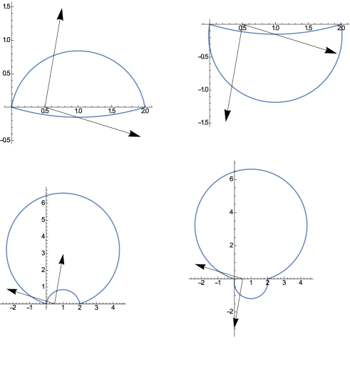
Figure 1: The four closed contours (blue) with cusps, formed out of circular segments, as images of rays (black), starting at (q,0) with q=0.5. Note the difference in scale between the first and second line.

Appendix B

In this appendix we review the calculation for a cusp with straight legs based on [8], [19]. Furthermore, we present an alternative representation of the cusp anomalous dimension in terms of a hypergeometric function and comment on a parameterisation of the problem, more convenient for our discussion in the main text.

Due to the dilatation symmetry of a cusp located at the origin between two straight legs extending to infinity, one can describe the $r$-coordinate of the string surface by the ansatz

$$r~{}=~{}\frac{\rho}{f(\varphi)}~{},$$ (73)

where $\rho,\varphi$ are polar coordinates in the $(x_{1},x_{2})$-plane of the $AdS$ boundary at $r=0$, i.e.

$$x_{1}~{}=~{}\rho~{}\mbox{cos}~{}\varphi~{},~{}~{}~{}~{}~{}x_{2}~{}=~{}\rho~{}\mbox{sin}~{}\varphi~{}.$$ (74)

Then the determinant of the induced metric on the surface turns out to be

$$h~{}=~{}\frac{f^{4}+f^{2}+(f^{\prime})^{2}}{\rho^{2}}~{},$$ (75)

and, in virtue of this factorisation of the $\rho$ and $\varphi$ dependence, the minimal surface condition (equation of motion) is an ordinary differential equation for $f(\varphi)$ with boundary conditions $f(0)=f(\theta)=\infty$ ($\theta$ cusp angle)

$$f^{\prime\prime}(f^{4}+f^{2})-2(f^{\prime})^{2}(f+2f^{3})-f^{3}(1+f^{2})(1+2f^{2})~{}=~{}0~{}.$$ (76)

Instead of solving this second order equation directly, it is more convenient to use the conservation law related to the lack of any explicit $\varphi$-dependence in (75)

$$E~{}=~{}f_{0}\sqrt{1+f_{0}^{2}}~{}=~{}\frac{f^{4}+f^{2}}{\sqrt{f^{4}+f^{2}+(f^{\prime})^{2}}}~{},$$ (77)

with $f_{0}=f(\theta/2)$ denoting the minimal value of $f$ in $\varphi\in(0,\theta)$. Now integration yields

$$\varphi~{}=~{}E~{}\int_{f}^{\infty}\frac{df}{\sqrt{(f^{4}+f^{2})^{2}-E^{2}(f^{4}+f^{2})}}~{}.$$ (78)

This holds for $0<\varphi<\theta/2$, and furthermore one has $f(\varphi)=f(\theta-\varphi)$.

In particular the equation

$$\theta~{}=~{}2E~{}\int_{f_{0}}^{\infty}\frac{df}{\sqrt{(f^{4}+f^{2})^{2}-E^{2}(f^{4}+f^{2})}}~{}$$ (79)

fixes the relation between $f_{0}$ and the cusp angle $\theta$. The function $\theta(f_{0})$ is monotonically decreasing, $\theta(0)=\pi,~{}~{}\theta(\infty)=0$. The estimate of this equation and (77) for large $f_{0}$ yields

$$\theta~{}=~{}\frac{2\pi^{1/2}\Gamma(\frac{3}{4})}{\Gamma(\frac{1}{4})}~{}f_{0}^{-1}~{}+~{}{\cal O}(f_{0}^{-3})~{}.$$ (80)

Expanding the integrand in eq.(78) for large $f$ (but fixed $f_{0}$) one gets

$$\frac{\varphi}{E}~{}=~{}\frac{1}{3}f^{-3}-\frac{1}{5}f^{-5}+\frac{1}{7}(1+\frac{E^{2}}{2})f^{-7}+{\cal O}(f^{-9})~{}.$$ (81)

The inversion of (81) is

$$\frac{1}{f(\varphi)}~{}=~{}\Big{(}\frac{3\varphi}{E}\Big{)}^{1/3}~{}+~{}\frac{1}{5}\cdot\frac{3\varphi}{E}~{}+~{}\frac{6-25E^{2}}{350}\cdot\Big{(}\frac{3\varphi}{E}\Big{)}^{5/3}~{}+~{}{\cal O}(\varphi^{7/3})~{}.$$ (82)

For use in the main text we note that

$$F(\varphi):=\frac{1}{f(\varphi)}~{}$$ (83)

defines a function which has an ordinary Taylor expansion in $x=\varphi^{1/3}$ around $x=0$. Expressing the equation of motion (76) in terms of $F(\varphi)$ it looks like

$$2~{}(F^{\prime})^{2}~{}+~{}(1+F^{2})~{}(2+F^{2}+FF^{\prime\prime})~{}=~{}0~{}.$$ (84)

For the regularised area, defined with the cutoffs $r=\rho/f(\varphi)>\epsilon$ and $\rho<L$, one gets

$$A_{\epsilon,L} = \int d\rho~{}d\varphi~{}\frac{\sqrt{f^{4}+f^{2}+(f^{\prime})^{2}}}{\rho}$$ (85)

$$= \frac{2L}{\epsilon}~{}+~{}\Gamma_{\mbox{\tiny cusp}}(\theta)~{}\mbox{log}\frac{\epsilon}{L}~{}+~{}A_{0}(\theta)~{}+~{}\dots~{}.$$

The dots denote terms vanishing for $\epsilon\rightarrow 0$ and

$$\Gamma_{\mbox{\tiny cusp}}(\theta)~{}=~{}2f_{0}~{}-~{}2\int_{f_{0}}^{\infty}\left(\sqrt{\frac{f^{4}+f^{2}}{f^{4}+f^{2}-E^{2}}}-1\right)df~{},$$ (86)

$$A_{0}(\theta)~{}=~{}2f_{0}~{}(\mbox{log}f_{0}~{}-~{}1)~{}-~{}2\int_{f_{0}}^{\infty}\mbox{log}f\left(\sqrt{\frac{f^{4}+f^{2}}{f^{4}+f^{2}-E^{2}}}-1\right)df~{}.$$ (87)

The substitution $f^{2}=f_{0}^{2}+z^{2}$ yields [19]

$$\Gamma_{\mbox{\tiny cusp}}(\theta)~{}=~{}\int_{-\infty}^{\infty}\left(1-\sqrt{\frac{1+z^{2}+f_{0}^{2}}{1+z^{2}+2f_{0}^{2}}}~{}\right)dz~{}.$$ (88)

Based on this integral we found a closed expression in terms of a hypergeometric function

$$\Gamma_{\mbox{\tiny cusp}}(\theta)~{}=~{}\frac{\pi}{2}\frac{f_{0}^{2}}{\sqrt{1+f_{0}^{2}}}~{}~{}_{2}F_{1}\Big{(}\frac{1}{2},\frac{3}{2},2,\frac{-f_{0}^{2}}{1+f_{0}^{2}}\Big{)}~{}.$$ (89)

This implies that $\Gamma_{\mbox{\tiny cusp}}$ for $\theta\rightarrow\pi$, i.e. $f_{0}\rightarrow 0$ goes to zero and for $\theta\rightarrow 0$ i.e. $f_{0}\rightarrow\infty$ grows linearly in $f_{0}$ with a factor $\frac{\sqrt{\pi}~{}\Gamma(3/4)}{2~{}\Gamma(5/4)}$.

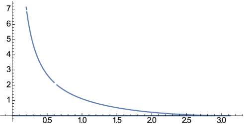
Figure 2: $\Gamma_{\mbox{\tiny cusp}}$ as a function of $\theta$, obtained with $f_{0}$ as parameter in ParametricPlot.

Appendix C

This appendix is devoted to the $\epsilon\rightarrow 0$ asymptotics of $A_{\epsilon}^{(j,1)}$, as defined in (18). We start with

$$A_{\epsilon}^{(j,1)} = 2~{}\int_{f_{0}}^{f_{\epsilon}^{(j)}}df~{}\left(\sqrt{\frac{f^{4}+f^{2}}{f^{4}+f^{2}-E^{2}}}-1\right)~{}\mbox{log}N_{\epsilon}^{(j)}(q,f)$$ (90)

$$+~{}2~{}\int_{f_{0}}^{f_{\epsilon}^{(j)}}df~{}\mbox{log}N_{\epsilon}^{(j)}(q,f)~{}.$$

In the first term of the above equation the factor in big brackets is ${\cal O}(1/f^{4})$ for large $f$. Let us split the integration region into the intervals $(f_{0},T_{j}/\epsilon^{1/2})$ and $(T_{j}/\epsilon^{1/2},f^{(j)}_{\epsilon})$. Then in the first interval $\mbox{log}N_{\epsilon}^{(j)}(q,f)$ approaches $\mbox{log}2$. This is no longer true in the second interval, but due to the fast vanishing of the factor in big brackets the corresponding integral drops out for $\epsilon\rightarrow 0$. This implies

$$A_{\epsilon}^{(j,1)} = 2~{}\mbox{log}2~{}\int_{f_{0}}^{\infty}df~{}\left(\sqrt{\frac{f^{4}+f^{2}}{f^{4}+f^{2}-E^{2}}}-1\right)$$ (91)

$$+~{}2~{}\int_{f_{0}}^{f_{\epsilon}^{(j)}}df~{}\mbox{log}N_{\epsilon}^{(j)}(q,f)~{}+~{}\mbox{{\tiny\cal O}}(1)~{}.$$

Denoting the second line of the last equation by $J_{\epsilon}$ and using the same splitting of the integration interval, we get after the substitution $x=qf\epsilon$ with (15) and (2)

$$J_{\epsilon}=~{}J_{\epsilon}^{\mbox{\tiny lower}}~{}+~{}J_{\epsilon}^{\mbox{\tiny upper}}~{}=~{}\frac{2}{q\epsilon}~{}\left(\int_{q\epsilon f_{0}}^{qT\epsilon^{1/2}}~{}+~{}\int^{qT-\epsilon q^{2}}_{qT\epsilon^{1/2}}\right)~{}\mbox{log}N_{\epsilon}(q,\frac{x}{q\epsilon})~{}dx~{}.$$ (92)

Then in $J_{\epsilon}^{\mbox{\tiny lower}}$ the integration variable $x$ is small, allowing an expansion of $\mbox{log}N_{\epsilon}(q,\frac{x}{q\epsilon})$ in terms of $x$. This yields

$$J_{\epsilon}^{\mbox{\tiny lower}}~{}=~{}\frac{2T}{\epsilon^{1/2}}~{}\mbox{log}2~{}-~{}2f_{0}~{}\mbox{log}2~{}-~{}\frac{4}{q\epsilon}~{}\int_{q\epsilon f_{0}}^{qT\epsilon^{1/2}}x~{}\mbox{cos}\big{(}\varphi\big{(}\frac{x}{q\epsilon}\big{)}\pm\gamma\big{)}~{}dx~{}+~{}\mbox{{\tiny\cal O}}(1)~{}.$$ (93)

In $J_{\epsilon}^{\mbox{\tiny upper}}$ the argument of $\varphi(f)$, i.e. $f=x/(q\epsilon)$, tends to infinity where $\varphi=0.$ This approach to zero is fast enough to justify

$$J_{\epsilon}^{\mbox{\tiny upper}}~{}=~{}\frac{2}{q\epsilon}~{}\int^{qT-\epsilon q^{2}}_{qT\epsilon^{1/2}}dx~{}\mbox{log}\Big{(}1-2x~{}\mbox{cos}\gamma+\sqrt{1-4x~{}\mbox{cos}\gamma-4x^{2}\mbox{sin}^{2}\gamma}~{}\Big{)}~{}+~{}\mbox{{\tiny\cal O}}(1)~{}.$$ (94)

Writing this as an integral over $(0,qT)$ minus integrals over $(0,qT\epsilon^{1/2})$ and over $(qT-\epsilon q^{2},qT)$ we get

$$J_{\epsilon}^{\mbox{\tiny upper}} = \frac{2}{q\epsilon}~{}\int^{qT}_{0}dx~{}\mbox{log}\Big{(}1-2x~{}\mbox{cos}\gamma+\sqrt{1-4x~{}\mbox{cos}\gamma-4x^{2}\mbox{sin}^{2}\gamma}~{}\Big{)}$$ (95)

$$~{}-~{}2q~{}\mbox{log}\Big{(}1-2qT~{}\mbox{cos}\gamma+\sqrt{1-4qT~{}\mbox{cos}\gamma-4q^{2}T^{2}\mbox{sin}^{2}\gamma}~{}\Big{)}$$

$$~{}-\frac{2T}{\epsilon^{1/2}}~{}\mbox{log}2~{}+~{}\frac{4}{q\epsilon}~{}\int_{0}^{qT\epsilon^{1/2}}x~{}\mbox{cos}\gamma~{}dx~{}+~{}\mbox{{\tiny\cal O}}(1)~{}.$$

In the sum $J_{\epsilon}^{\mbox{\tiny lower}}+J_{\epsilon}^{\mbox{\tiny upper}}$ the terms $\propto 1/\epsilon^{1/2}$ cancel. A further cancellation (up to vanishing terms) takes place for the last terms in (93) and (95). Then, using the integral

$$\int^{\frac{1-\mbox{\tiny cos}\gamma}{2~{}\mbox{\tiny sin}^{2}\gamma}}_{0}dx~{}\mbox{log}\Big{(}1-2x~{}\mbox{cos}\gamma+\sqrt{1-4x~{}\mbox{cos}\gamma-4x^{2}\mbox{sin}^{2}\gamma}~{}\Big{)}$$ (96)

$$~{}~{}~{}~{}~{}~{}~{}~{}~{}~{}~{}~{}~{}~{}~{}~{}~{}~{}~{}~{}~{}=~{}\frac{\gamma}{2~{}\mbox{sin}\gamma}~{}-~{}\frac{1+\mbox{log}(1+\mbox{cos}\gamma)}{4~{}\mbox{cos}^{2}\frac{\gamma}{2}}~{},$$

and inserting (93), (95) and (92) into (91) we get with $T_{j}$ given by (15)

$$A_{\epsilon}^{(j,1)} = \frac{2}{q\epsilon}~{}\left(\frac{\gamma_{j}}{2~{}\mbox{sin}\gamma_{j}}-\frac{1+\mbox{log}(1+\mbox{cos}\gamma_{j})}{4~{}\mbox{cos}^{2}\frac{\gamma_{j}}{2}}\right)$$ (97)

$$~{}+2~{}\mbox{log}2~{}\left(\int_{f_{0}}^{\infty}df~{}\left(\sqrt{\frac{f^{4}+f^{2}}{f^{4}+f^{2}-E^{2}}}-1\right)~{}-f_{0}\right)$$

$$~{}-2q~{}\mbox{log}\Big{(}\frac{1-\mbox{cos}\gamma_{j}}{\mbox{sin}^{2}\gamma_{j}}\Big{)}~{}+~{}\mbox{{\tiny\cal O}}(1)~{}.$$

Appendix D

In this appendix we give arguments for the ansatz for the coordinates (41),(42) based on the experience with the explicit example in section 2. If we would take $s(\varphi)=0$, the variable $\varphi$ would have the meaning of an angle in the $(x_{1},x_{2})$-plane. Instead we want to argue, that in a well adapted coordinate system $\psi=\rho s(\varphi)+\varphi$ has this meaning. From the mapping pattern of section 2 we have

$$\frac{y_{1}-1/q}{y_{2}}~{}=~{}\mbox{cot}(\pi-\gamma_{1}-\psi)~{}=~{}-\mbox{cot}(\gamma_{1}+\psi)~{}.$$ (98)

On the other side the explicit mapping formulas (9) yield

$$\frac{y_{1}-1/q}{y_{2}}~{}=~{}-~{}\mbox{cot}(\gamma_{1}+\varphi)~{}-~{}\frac{\rho(1+1/f^{2})}{q~{}\mbox{sin}(\gamma_{1}+\varphi)}~{}.$$ (99)

Using (82) a comparison of these two expressions gives

$$\psi~{}=~{}-\Big{(}\frac{3}{E}\Big{)}^{2/3}\frac{\rho}{q}~{}\big{(}\varphi^{2/3}+{\cal O}(\varphi)\big{)}~{}+~{}\varphi~{}+~{}{\cal O}(\rho,\varphi^{4/3})~{}.$$ (100)

Note that $\rho$ as used in section 2 is proportional to the radius variable in the sense of section 3 up to higher order corrections, which are not essential in this discussion, whose only purpose is to see the emergence of the structure $\varphi+\mbox{ factor}\times\rho\varphi^{2/3}$.

To get an impression of the effect of working with $s(\varphi)$ as described in section 3 for a generic example, i.e. not related to section 2, we have added figure 3.

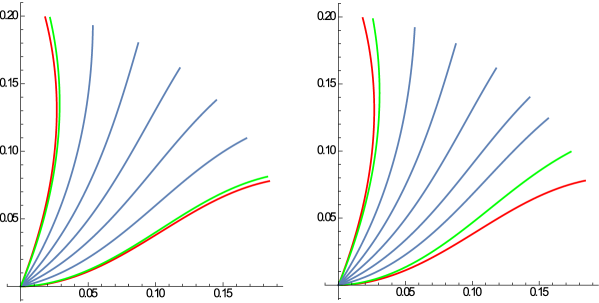
Figure 3: Example for $\theta=1.2$ and $\phi_{1}(\rho)=5\rho-15\rho^{2}~{},~{}~{}\phi_{2}=1.2+\rho+2\rho^{2}$ (red curves). Lines of constant $\varphi$ in step size 0.2 are shown in blue. Green lines show the first steps with size 0.02. On the left we see the situation for $s=0$, on the right for $s(\varphi):=a_{1}\varphi^{2/3}(1-\varphi/\theta)^{10}+a_{2}(\theta-\varphi)^{2/3}(\varphi/\theta)^{10}$. $a_{1}$,$a_{2}$ are adapted as described in the text.

Appendix E

Here we want to comment on some properties of the differential equation for $F_{2}(\varphi)$, see (44). As mentioned in the main text, for $F_{1}$ in (3)-(47) we can take $F$ from appendix B. Furthermore, with (77),(83) we get

$$F^{\prime}(\varphi)~{}=~{}\pm\frac{\sqrt{(1+F^{2})(1+F^{2}-E^{2}F^{4})}}{EF^{2}}~{},~{}~{}~{}~{}F^{\prime\prime}(\varphi)~{}=~{}-\frac{2+2F^{2}+E^{2}F^{6}}{E^{2}F^{5}}~{}.$$ (101)

The plus sign for $F^{\prime}$ applies to $\varphi\in(0,\theta/2)$ and the minus to $\varphi\in(\theta/2,\theta)$. The relation between $\varphi$ and $F$ is one to one in both half-intervals. The constant $E$ is related to the maximum of $F$ (i.e. $F_{0}=F(\theta/2)=1/f_{0}$) via

$$E~{}=~{}\frac{\sqrt{1+F_{0}^{2}}}{F_{0}^{2}}~{}.$$ (102)

Due to $F(\theta-\varphi)=F(\varphi)$ we have $G(\theta-\varphi)=G(\varphi)$ and $G_{1}(\theta-\varphi)=-G(\varphi)$. Thus the homogeneous equation related to (44) has both a symmetric as well as an antisymmetric solution. The equation is regular inside the whole interval $\varphi\in(0,\theta)$, but is singular at its boundary points.

Via

$$\tilde{F}_{2}(F)~{}:=~{}F_{2}(\varphi)$$ (103)

we can replace (44) by a differential equation with respect to $F$

$$\tilde{F}^{\prime\prime}_{2}(F)~{}+~{}g_{1}(F)\tilde{F}^{\prime}_{2}(F)~{}+~{}g(F)\tilde{F}_{2}(F)~{}+~{}m(F)~{}=~{}0~{},$$ (104)

with

$$g(F) = \frac{2+10F^{2}+6F^{4}-(2+10E^{2})F^{6}}{(F+F^{3})^{2}(E^{2}F^{4}-1-F^{2})}~{},$$

$$g_{1}(F) = \frac{2-F^{4}\big{(}2-E^{2}(F^{2}-4)\big{)}}{(F+F^{3})(1+F^{2}-E^{2}F^{4})}~{},$$

$$m(F) = \frac{M\big{(}\varphi(F)\big{)}}{(dF/d\varphi)^{2}}~{}.$$ (105)

Remarkably, the coefficient functions of the homogeneous equation are now explicit known rational functions of $F$. Besides other benefits, this considerably simplifies the evaluation of numerical solutions.

The equation (104) is regular inside $F\in(0,F_{0})$ and has regular singularities at the boundaries. The one at $F_{0}$ is an artefact of the change of variables from $\varphi$ to $F$. The corresponding Frobenius series for the homogeneous equation are power series in $\sqrt{F_{0}-F}$ or in $(F_{0}-F)$, related to odd or even power series in $(\varphi-\theta/2)$ for $F_{2}(\varphi)$.

Near $F=0$ we have $g(F)=-2/F^{2}\times(1+{\cal O}(F^{2}))$ and $g_{1}(F)=2/F\times(1+{\cal O}(F^{2}))$. Therefore, the indicial equation for solving the homogeneous equation by the Frobenius method is $\alpha(\alpha-1)+2\alpha-2=0$. Its solutions are $\alpha=-2$ and $\alpha=1$, corresponding to $\tilde{F}_{2}(F)=F^{-2}(1+\dots)$ and $\tilde{F}_{2}(F)=F(1+\dots)$, where in both cases the dots stand for power series in $F^{2}$.

What does this imply for the original differential equation w.r.t. $\varphi$, i.e. (44)? The just discussed behaviour at $F\rightarrow 0$ fixes via (82)-(83) the behaviour of the solutions of the homogeneous version of (44), both at $\varphi\rightarrow 0$ and $\varphi\rightarrow\theta$. On both boundary points of the $\varphi$-interval we have a vanishing and a diverging solution. From the previous discussion of the behaviour around the midpoint $\theta/2$ we also know, that there are symmetric as well as antisymmetric solutions. However, a symmetric or antisymmetric solution, vanishing both at $\varphi=0$ and $\varphi=\theta$, could only exist, if the spectrum of eigenvalues of the differential operator in (44) would contain the value zero. Certainly, if at all, this could happen only at special values of the parameter $F_{0}$, which contains the information on $\theta$.

The upshot of this discussion so far is, that for a generic value of $\theta$ the homogeneous equation related to (44) has two independent solutions $y_{1}(\varphi)$ and $y_{2}(\varphi)$ with

$$y_{1}(\varphi) \propto \varphi^{-\frac{2}{3}}~{},~{}~{}~{}~{}~{}~{}~{}~{}~{}~{}y_{2}(\varphi)~{}\propto~{}\varphi^{\frac{1}{3}}~{},~{}~{}~{}~{}~{}~{}~{}~{}~{}~{}~{}~{}~{}~{}~{}~{}\varphi\rightarrow 0$$

$$y_{1}(\varphi) \propto (\theta-\varphi)^{\frac{1}{3}}~{},~{}~{}~{}~{}y_{2}(\varphi)~{}\propto~{}(\theta-\varphi)^{-\frac{2}{3}}~{},~{}~{}~{}~{}~{}~{}~{}~{}\varphi\rightarrow\theta~{}.$$ (106)

Let us now proceed to the construction of a solution for the full inhomogeneous equation (44) by the method of varying the constants, i.e. starting with the ansatz

$$F_{2}(\varphi)~{}=~{}v_{1}(\varphi)~{}y_{1}(\varphi)~{}+~{}~{}v_{2}(\varphi)~{}y_{2}(\varphi)~{}.$$ (107)

Then the coefficient functions $v_{j}(\varphi)$ have to obey the equations

$$v^{\prime}_{1}(\varphi)~{}=~{}\frac{M(\varphi)}{W(\varphi)}~{}y_{2}(\varphi)~{},~{}~{}~{}~{}~{}~{}~{}~{}v^{\prime}_{2}(\varphi)~{}=~{}-\frac{M(\varphi)}{W(\varphi)}~{}y_{1}(\varphi)~{}.$$ (108)

Their solutions are

$$v_{1}(\varphi)~{}=~{}v_{1}(0)~{}+~{}\int_{0}^{\varphi}\frac{M}{W}~{}y_{2}d\varphi~{},~{}~{}~{}v_{2}(\varphi)~{}=~{}v_{2}(0)~{}-~{}\int_{0}^{\varphi}\frac{M}{W}~{}y_{2}d\varphi~{}.$$ (109)

Here $W(\varphi)$ denotes the Wronskian. It is given by

$$W(\varphi)~{}=~{}\mbox{exp}\left(-\int^{\varphi}G_{1}~{}d\varphi\right)~{}=~{}\mbox{const}\cdot\frac{(1+F^{2})^{3}}{F^{4}}~{}.$$ (110)

From (110),(82) and (50) with (54) and its analog for $\varphi\rightarrow\theta$ we see that the quotient $M/W$ at both boundary points of the $\varphi$-interval tends to nonzero constants. Therefore we get from (109) and (106) near $\varphi=0$ and $\varphi=\theta$

$$F_{2}(\varphi) = v_{1}(0)(\varphi^{-\frac{2}{3}}+\dots)+v_{2}(0)(\varphi^{\frac{1}{3}}+\dots)+(b_{1}+b_{2})(\varphi^{\frac{2}{3}}+\dots)~{},$$ (111)

$$F_{2}(\varphi) = v_{1}(\theta)\big{(}(\theta-\varphi)^{\frac{1}{3}}+\dots\big{)}+v_{2}(\theta)\big{(}(\theta-\varphi\big{)}^{-\frac{2}{3}}+\dots)+(\hat{b}_{1}+\hat{b}_{2})\big{(}(\theta-\varphi)^{\frac{2}{3}}+\dots\big{)}.$$

The $b_{j}$ and $\hat{b}_{j}$ are some constants.

Now vanishing $F_{2}$ at both ends of the $\varphi$-interval requires

$$v_{1}(0)~{}=~{}v_{2}(\theta)~{}=~{}0~{}.$$ (112)

Using (109) this can be translated in conditions exclusively formulated at one and the same endpoint, e.g. at $\varphi=0$

$$v_{1}(0)~{}=~{}0~{},~{}~{}~{}~{}~{}v_{2}(0)~{}=~{}\int_{0}^{\theta}\frac{M}{W}~{}y_{1}~{}d\varphi~{}.$$ (113)

Note that $v_{1}(0)$ and $v_{2}(0)$ are just the constants $B_{1}$ and $B_{2}$ in formula (3) of the main text.

Appendix F

Here we discuss the asymptotic evaluation of $A_{\epsilon,1}^{\tiny\mbox{c},0}(\rho_{0})$ needed in formula (62) of the main text. One of our aim is the identification of $\Gamma_{\mbox{\tiny cusp}}(\theta)$, defined in equation (86) of appendix B. Therefore, we replace the integration variable $\varphi$ by $f=1/F$ as used in that appendix

$$L_{1}(\varphi)~{}d\varphi~{}=~{}\sqrt{\frac{f^{4}+f^{2}}{f^{4}+f^{2}-E^{2}}}~{}df~{}.$$ (114)

Then

$$~{}A_{\epsilon,1}^{\tiny\mbox{c},0}(\rho_{0}) = \int_{\rho<\rho_{0},~{}~{}\rho/f+\rho^{2}F_{2}+{\cal O}(\rho^{3})>\epsilon}~{}\frac{1}{\rho}~{}\sqrt{\frac{f^{4}+f^{2}}{f^{4}+f^{2}-E^{2}}~{}}~{}d\rho df$$ (115)

$$= \int_{f_{0}}^{f_{\mbox{\tiny max}}(\epsilon)}\left(\sqrt{\frac{f^{4}+f^{2}}{f^{4}+f^{2}-E^{2}}~{}}-1\right)df\int_{\rho_{\epsilon}(f)}^{\rho_{0}}\frac{d\rho}{\rho}$$

$$+\int_{f_{0}}^{f_{\mbox{\tiny max}}(\epsilon)}df\int_{\rho_{\epsilon}(f)}^{\rho_{0}}\frac{d\rho}{\rho}~{},$$

with

$$\rho_{\epsilon}(f)~{}=~{}\frac{\sqrt{a^{2}+4\epsilon~{}afB_{2}~{}}-a}{2B_{2}}~{},~{}~{}~{}f_{\mbox{\tiny max}}(\epsilon)~{}=~{}\frac{\rho_{0}+\frac{B_{2}}{a}\rho_{0}^{2}+{\cal O}(\rho_{0}^{3})}{\epsilon}~{}.$$ (116)

Use has been made of the asymptotics of $F_{2}$ for small $\varphi$, i.e. large $f$, see (3),(82) and (48).

Let us call the second and third line of (115) $I_{1}$ and $I_{2}$ respectively. Then

$$I_{1}~{}=~{}\int_{f_{0}}^{f_{\mbox{\tiny max}}(\epsilon)}df~{}\left(\sqrt{\frac{f^{4}+f^{2}}{f^{4}+f^{2}-E^{2}}~{}}-1\right)~{}\mbox{log}\frac{2\rho_{0}B_{2}}{\sqrt{a^{2}+4\epsilon aB_{2}f~{}}-a}~{}.$$ (117)

For $f$ fixed one has $\rho_{\epsilon}(f)=\epsilon f+{\cal O}(\epsilon^{2})$. However, since the upper integration boundary is $\propto 1/\epsilon$, one has to use this simplification with caution. In the case of $I_{1}$ the factor multiplying the logarithm fastly goes to zero $\propto 1/f^{4}$, ensuring the finiteness of the integral and allowing the use of the simplified expression for $\rho_{\epsilon}(f)$. This yields

$$I_{1}~{}=~{}\int_{f_{0}}^{\infty}df~{}\left(\sqrt{\frac{f^{4}+f^{2}}{f^{4}+f^{2}-E^{2}}~{}}-1\right)~{}\mbox{log}\frac{\rho_{0}}{\epsilon}~{}+~{}{\cal O}(1)~{}.$$ (118)

$I_{2}$ diverges for $\epsilon\rightarrow 0$. Here the use of the same simplification for $\rho_{\epsilon}(f)$ is not justified. But due to its simpler total integrand it can be performed explicitly

$$I_{2} = (f_{\mbox{\tiny max}}(\epsilon)-f_{0})~{}\mbox{log}\Big{(}\frac{2\rho_{0}B_{2}}{a}\Big{)}~{}-~{}\int_{f_{0}}^{f_{\mbox{\tiny max}}(\epsilon)}df~{}\mbox{log}\Big{(}\sqrt{1+\frac{4\epsilon B_{2}}{a}~{}f~{}}-1\Big{)}$$ (119)

$$~{}=~{}\frac{1}{\epsilon}~{}\Big{(}\rho_{0}+\frac{B_{2}}{2a}\rho_{0}^{2}+{\cal O}(\rho_{0}^{3})\Big{)}~{}+~{}f_{0}~{}\mbox{log}\epsilon~{}+~{}{\cal O}(1)~{}.$$

The sum $I_{1}+I_{2}$ is then (with use of (86))

$$A_{\epsilon,1}^{\tiny\mbox{c},0}(\rho_{0})~{}=~{}\frac{1}{\epsilon}~{}\Big{(}\rho_{0}+\frac{B_{2}}{2a}\rho_{0}^{2}+{\cal O}(\rho_{0}^{3})\Big{)}~{}+~{}\frac{1}{2}~{}\Gamma_{\mbox{\tiny cusp}}(\theta)~{}\mbox{log}\epsilon~{}+~{}{\cal O}(1)~{}.$$ (120)