Early warning of large volatilities based on recurrence interval analysis in Chinese stock markets

Abstract

Being able to forcast extreme volatility is a central issue in financial risk management. We present a large volatility predicting method based on the distribution of recurrence intervals between volatilities exceeding a certain threshold $Q$ for a fixed expected recurrence time $\tau_{Q}$. We find that the recurrence intervals are well approximated by the $q$-exponential distribution for all stocks and all $\tau_{Q}$ values. Thus a analytical formula for determining the hazard probability $W(\Delta t|t)$ that a volatility above $Q$ will occur within a short interval $\Delta t$ if the last volatility exceeding $Q$ happened $t$ periods ago can be directly derived from the $q$-exponential distribution, which is found to be in good agreement with the empirical hazard probability from real stock data. Using these results, we adopt a decision-making algorithm for triggering the alarm of the occurrence of the next volatility above $Q$ based on the hazard probability. Using a “receiver operator characteristic” (ROC) analysis, we find that this predicting method efficiently forecasts the occurrance of large volatility events in real stock data. Our analysis may help us better understand reoccurring large volatilities and more accurately quantify financial risks in stock markets. JEL classification: C14

1 Introduction

Predicting extreme volatility events in financial markets is essential when estimating risk. A standard approach to extreme event prediction is to find the precursory patterns prior to an extreme event or to quantify the probability that a given pattern is a precursor to an extreme event [1, 2]. [3, 4] propose a new method based on the statistics of the recurrence intervals between events exceeding a threshold to determine the risk probability $W(\Delta t|t)$ that an extreme event will occur within the next $\Delta t$ intervals when the last extreme event occurred $t$ periods ago. They find that when examining real market data and model data with a low level of noise the predicting method based on recurrence interval analysis produces a better performance forecast than the method based on precursor pattern recognition [3, 4].

Understanding of the recurrence interval, defined as the waiting time between consecutive events with values greater than a predefined threshold $Q$, is essential in uncovering the underlying laws governing extreme events in many fields. Recurrent interval analysis has been carried out on many kinds of time series in predicting the probability that an extreme event will occur, including records of climate [5, 6], seismic activities [7], energy dissipation rates of three-dimensional turbulence [8], heartbeat intervals in medical science [9], precipitation and river runoff [10], internet traffic [11, 12], financial volatilities [13, 14], equity returns [15, 16, 17, 3, 18, 19, 20, 21, 22], and trading volumes [23, 24, 25]. An improved method of estimating value at risk (VaR) in financial markets has been proposed based on the recurrence interval between the last two returns below $-Q$. This method is significantly more accurate than traditional estimates based on the overall or local return distributions [3, 19].

To accurately estimate the risk probability and the VaR based on recurrence interval analysis we need the set of distribution and memory behavior of the recurrence time between extreme events. It is found that the recurrence intervals of the time series in many different fields exhibit fat-tailed distributions and long- and short-range memories, indicating that extreme events are not described by the Poisson process. Unlike long- and short-range memory behaviors, which are easily testable using conditional distribution analysis and the DFA method, the distribution form of recurrence intervals is still elusive. For example, in financial markets the recurrence intervals of different data types (return, volatility, and trading volume), different data resolutions (minute-by-minute and daily), and different markets fit different distributions, including power-law, stretched exponential, and $q$-exponential. It has been found that the recurrence interval distribution above a fixed threshold has a power-law tail for the daily volatilities in Japanese market [26, 13], the minute-by-minute volatilities in Korean market [27] and Italian market [28], the daily returns in US stock markets [16, 17, 3], the minute-by-minute returns in Chinese markets [18], and the minute-by-minute trading volume in US markets [25] and Chinese markets [24]. A number of studies ranging from daily to high-frequency data and from developed to emerging markets [29, 30, 31, 32, 33, 34, 35, 36, 14], have also reported that the distribution of the recurrence intervals of financial volatility is a stretched exponential. Reference [22] reports that in Chinese markets the recurrence time between returns above a given positive threshold or below a negative threshold for the index spot and futures fits a stretched exponential distribution. The recurrence intervals between losses in financial markets were recently found to fit a $q$-exponential distribution [19, 37].

In this paper we describe the datasets in Sec. 2, present the theoretical framework for predicting large volatilities in Sec. 3, determine the distribution of the recurrence intervals between large volatilities in Sec. 4, and report the hazard probability results and predicting algorithm performance in Sec. 5. In Sec. 6 we summarize our findings.

2 Data description

To carry out a detailed recurrence interval analysis of Chinese stock markets, we include as many Chinese stocks in our analyzing sample as possible. The minute-by-minute price data of all stocks in the Chinese markets are extracted from the RESSET financial database. The extracting period is from 26 July 1999 to 30 December 2011, which is the maximum spanning period allowed in the RESSET database. To ensure that the recurrent interval results between the top 1% volatilities will have more than 1,000 data points, we select only those stocks that have a minimum of two years of trading records. Having this large a sample size lowers the error rate when we use a maximum likelihood estimation to fit the distributions. Finally, we have 1891 stocks in our sample, which include 853 A-shares, 54 B-shares, and 63 ChiNext shares in the Shenzhen market, and 867 A-shares and 54 B-shares in the Shanghai market.

3 Framework of predicting large volatilities

3.1 Hazard probability $W(\Delta t|t)$

We use the hazard probability $W(\Delta t|t)$ to forecast the occurrance of large volatility events. The $W(\Delta t|t)$ is the probability that there will be additional waiting time $\Delta t$ before another large volatility event occurs when the previous large volatility event occurred $t$ time ago. This probability is the key early-warning measurement for the occurrence of extreme volatilities. The early warning is triggered when the probability $W(\Delta t|t)$ is greater than a predefined alarm threshold. We can theoretically derive this hazard probability if we have the distribution of the time intervals between consecutive extreme volatilities, which are defined as the volatilities that exceed a given threshold $Q$.

Using the probability density $p(t)$ of the recurrence intervals between the extreme volatilities, if the time elapsed since the last extreme event is $t$, we want to determine the probability density function $p(\Delta{t}|t)$ that quantifies the additional waiting time $\Delta{t}$ until the next extreme event. Using the Bayes theorem for conditional probabilities, the probability that an event A occurs, given the knowledge of an event B, is simply the quotient of the probability of the event A without constraint and the probability of event B [38],

$$p(A|B)=\frac{p(AB)}{p(B)},$$ (1)

where $p(AB)=p(t+\Delta{t})$ is the probability that no event occurs from 0 to $t$ and that an event occurs at $t+\Delta{t}$, and $p(B)=\int_{t}^{\infty}p(s)ds$ is the probability that no event occurs from 0 to $t$. Thus we have

$$p(\Delta{t}|t)=\frac{p(t+\Delta{t})}{\int_{t}^{\infty}p(s)ds}.$$ (2)

Thus the hazard probability $W(\Delta{t},t)$ that an extreme event will occur after a short time $\Delta{t}\ll t$ since the occurrance of the previous extreme event can be expressed

$$W(\Delta{t}|t)=\frac{\int_{t}^{t+\Delta{t}}p(t)dt}{\int_{t}^{\infty}p(t)dt}.$$ (3)

3.2 Predicting algorithm

For a given distribution $p(t)$ of the recurrence intervals between extreme volatilities, the formula for $W(\Delta{t}|t)$ can be obtained using equation (3). If $\Delta t=1$ for $W(\Delta{t}|t)$, the hazard probability and a decision-making algorithm can be used to predict large volatilities [4]. To trigger an early warning that a large volatility is about to occur, we set a threshold $Q_{p}$ for the hazard probability. When the hazard probability exceeds $Q_{p}$, an alarm that a large volatility will occur during the next time point is activated. We next estimate the $Q_{p}$ parameter, which is the maximum correct prediction rate when the maximum false-alarm tolerance is set.

To determine $Q_{p}$ we estimate the correct prediction and false alarm rates for each $Q_{p}$ in the range of $[0,1]$. We then plot the correct prediction rate with respect to the false alarm rate and get the “receiver operator characteristic” (ROC) curve [3, 11, 9, 4]. The ROC curve is used to quantify prediction efficiency. The satisfied $Q_{p}$ corresponds to the point at which the false alarm rate equals the tolerant alarm level on the ROC curve.

To estimate the correct prediction and false alarm rates we generate for a given $Q_{p}$ two forecasting signals—alarms and non-alarms—at each time point. By comparing the forecasting signals with the real data, we obtain one of four outcomes at each time point [4], (i) a correct prediction of a large volatility event, (ii) a correct prediction of a non-large volatility event, (iii) a missed event, and (iv) a false alarm. By recording in our testing records how many times each outcome occurs we can estimate the correct prediction rate $D$ and the false alarm rate $A$ using

$$D=\frac{O_{11}}{O_{01}+O_{11}},~{}~{}A=\frac{O_{10}}{O_{00}+O_{10}},$$ (4)

where $O_{11}$ is the number of large volatility events that are correctly predicted, $O_{00}$ the number of non-large volatility events that are correctly predicted, $O_{01}$ the number of missed events, and $O_{10}$ the number of false alarms. All possible pairs of $(D,A)$ will be obtained if we vary the $Q_{p}$ range from 0 to 1.

By definition the ROC curve will be $D=A=1$ if $Q_{p}=0$ and $D=A=0$ if $Q_{p}=1$. Note that the ROC curve joins the point $(0,0)$ in the left bottom corner to the point $(1,1)$ in the right top corner. Note also that, for the random guess outcome, $D=A$, a straight line between the two corners. This occurs when there is no memory in the data. For a fixed value of $A$, the larger the value of the correct prediction rate, the better this algorithm performs.

4 Distribution of recurrence intervals between large volatilities

4.1 Definition of volatilities and recurrence intervals

For a given minute-by-minute price series $p(t)$, the minute-by-minute volatility $\omega(t)$ can be estimated [39] using

$$\omega(t)=|\ln p(t)-\ln p(t-1)|.$$ (5)

In order to eliminate the influence of the daily periodic patterns, we remove the intraday patterns from the volatility series $\omega(t)$ on each trading day,

$$\omega^{\prime}(s)=\omega(s)/A(s),$$ (6)

where $A(s)=\sum_{i}^{N}\omega(i,s)/N$. Here $\omega(i,s)$ represents the volatility at time $s$ on day $i$. The normalized volatility series $v(t)$ is then obtained by dividing $\omega^{\prime}(t)$ by its standard deviation,

$$v(t)=\frac{\omega^{\prime}(t)}{\sqrt{[\langle\omega^{\prime}(t)^{2}\rangle-\langle\omega^{\prime}(t)\rangle^{2}]}}.$$ (7)

The focus of our study is the recurrence interval between the normalized volatilities exceeding a predefined threshold $Q$. To compare the results between different stocks, we quantify $Q$ by its mean recurrence time $\tau_{Q}$. There is a one-to-one correspondence between $Q$ and $\tau_{Q}$, such that [23]

$$\frac{1}{\tau_{Q}}=\int_{Q}^{\infty}p(v){\rm{d}}v,$$ (8)

where $p(v)$ is the probability distribution of the volatility. Here we restrict $\tau_{Q}$ to a range of $[20,100]$. This range corresponds to the extreme volatilities from a top value of %5 to 1%, which is often considered in the risk estimation.

4.2 Distribution formula of recurrence intervals

To analytically determine the hazard probability we find the distribution that best approximates the recurrence interval distribution for all the stocks in our sample. We also determine whether the distribution parameters are dependent on the mean recurrence interval $\tau_{Q}$ and on whether the market is bear or bull. Previous research has indicated that the distribution of recurrence intervals between returns below a negative threshold $-Q$ depends only on the mean recurrence interval $\tau_{Q}$, and not on a specific asset or on the time resolution of the data [19, 37]. We first check whether the recurrence time between volatilities above a threshold $Q$ exhibits this behavior. Figure 1(a) shows the probability distribution of the recurrence intervals for 10 randomly chosen stocks. We transform the distribution curves of different $\tau_{Q}$ values by a factor to increase visibility. Note that for the same $\tau_{Q}$ value the recurrence time distributions of different stocks nearly overlap on the same curve. This means that the return intervals between volatilities that exceed a threshold $Q$ may exhibit a universal distribution for different stocks when $\tau_{Q}$ is fixed. We also want to know whether the distributions of different $\tau_{Q}$ values share the same pattern. Previous research indicates that these distributions are influenced only by the mean recurrence time $\tau_{Q}$ for return recurrence intervals [37]. Although the distributions in Fig. 1(a) seem to be different for different $\tau_{Q}$, if we scale the distribution using the mean recurrence time $\tau_{Q}$ the six distributions seem to be parallel [see Fig. 1(b)].

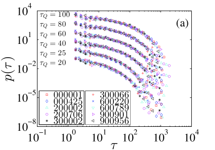
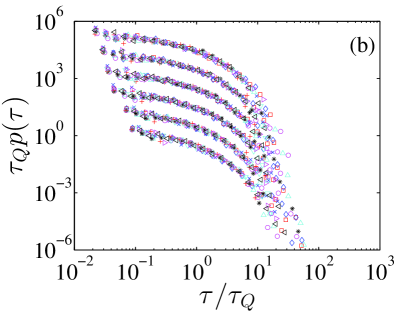
Figure 1: (color online). Probability distribution of the recurrence intervals for 10 randomly chosen stocks. For better visibility, the distribution curve of $\tau_{Q}=25$, $40$, $60$, $80$, and $100$ are shifted vertically by a factor of 10, 100, 1000, 10000, and 100000, respectively. (a) Original recurrence intervals. (b) Scaled recurrence intervals.

To quantitatively measure how the recurrence interval distributions vary with the mean interval $\tau_{Q}$, we need a suitable distributional formula for capturing the recurrence interval distribution. Previous research shows that the recurrence intervals can be fitted by the stretched distribution [29, 30, 31, 32, 35, 36, 22], the power-law distribution with an exponential cutoff [26, 13, 27, 28], and the $q$-exponential distribution [19, 37]. The Weibull distribution is usually comparable to the $q$-exponential distribution [40, 41], and we use both two-parameter and three-parameter Weibull distributions to fit the recurrence intervals in our analysis. The following are five candidate distributions: the stretched exponential distribution,

$$p(\tau)=a\exp[-(b\tau)^{\mu}],$$ (9)

the power-law distribution with an exponential cutoff,

$$p(\tau)=c\tau^{-\gamma-1}\exp(-k\tau),$$ (10)

the $q$-exponential distribution,

$$p(\tau)=(2-q)\lambda[1+(q-1)\lambda\tau]^{-\frac{1}{q-1}},$$ (11)

the two-parameter Weibull distribution,

$$p(\tau)=\frac{\zeta}{d}\left(\frac{\tau}{d}\right)^{\zeta-1}\exp\left[-\left(\frac{\tau}{d}\right)^{\zeta}\right],$$ (12)

and the three-parameter Weibull distribution,

$$p(\tau)=\frac{\zeta}{d}\left(\frac{\tau-\tau_{0}}{d}\right)^{\zeta-1}\exp\left[-\left(\frac{\tau-\tau_{0}}{d}\right)^{\zeta}\right].$$ (13)

To compare the recurrence interval distributions of different $\tau_{Q}$ values, we normalize the recurrence intervals by $\tau_{Q}$, i.e., $x=\tau/\tau_{Q}$. We obtain the five candidate distributions used to fit the normalized recurrence intervals by substituting $\tau=x\tau_{Q}$ into $f(x)=p(\tau)\tau_{Q}$, i.e.,

$$f(x)=a\bar{\tau}\exp[-(b\tau_{Q}x)^{\mu}],$$ (14)

$$f(x)=c\tau_{Q}^{-\gamma}x^{-\gamma-1}\exp(-k\tau_{Q}x),$$ (15)

$$p(\tau)=(2-q)(\lambda\tau_{Q})[1+(q-1)(\lambda\tau_{Q})\tau]^{-\frac{1}{q-1}},$$ (16)

$$f(x)=\frac{\zeta}{d/\tau_{Q}}\left(\frac{x}{d/\tau_{Q}}\right)^{\zeta-1}\exp\left[-\left(\frac{x}{d/\tau_{Q}}\right)^{\zeta}\right],$$ (17)

and

$$f(x)=\frac{\zeta}{d/\tau_{Q}}\left(\frac{x-\tau_{0}/\tau_{Q}}{d/\tau_{Q}}\right)^{\zeta-1}\exp\left[-\left(\frac{x-\tau_{0}/\tau_{Q}}{d/\tau_{Q}}\right)^{\zeta}\right].$$ (18)

We use the maximum likelihood estimation (MLE) method to estimate the parameters of the five distribution parameters. The details of fitting the stretched exponential distribution and the power-law distribution with an exponential cutoff are presented in the Appendix. Note that in the following analysis we fit only the scaled recurrence intervals.

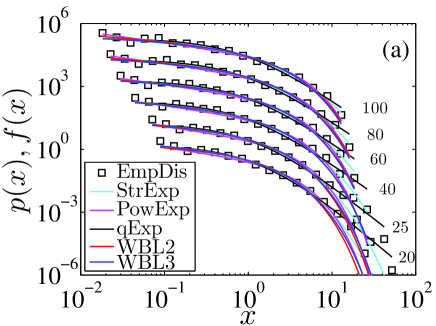
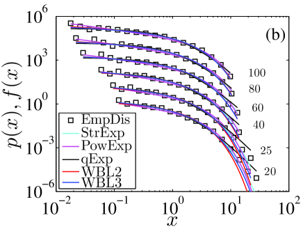
Figure 2: (color online). Plots of distribution fits to normalized recurrence intervals for two stocks. The open markers are the empirical distributions and the solid lines are the fits to the five candidate distributions. For better visibility, the curves of $\tau_{Q}=25$, $40$, $60$, $80$, and $100$ are shifted vertically by a factor of 10, 100, 1000, 10000, and 100000, respectively. (a) Stock 000001. (b) Stock 900956.

Figure 2 shows the empirical distributions and the fitting results of the five candidate distributions of the scaled recurrence intervals for two stocks, 000001 and 900956. Note that in the central regions of the distributions all five candidates agree with the empirical data. Note also that the $q$-exponential distribution better fits the distribution tail for all $\tau_{Q}$ than any other candidate distribution. To determine which distribution has the best performance, we utilize KS statistics to quantify the agreement between the empirical distribution and the fitting distributions. Figures 3(a) and 3(d) show the KS statistics of the five candidate distributions with respect to the mean recurrence time $\tau_{Q}$ for the two stocks. For stock 000001 the $q$-exponential distribution outperforms the other distributions and possesses the smallest KS statistics for all $\tau_{Q}$. For stock 900956 the $q$-exponential distribution is best when $\tau_{Q}\leq 60$, and the stretched exponential distribution is best when $\tau_{Q}>60$. Figure 3 shows plots of the characteristic parameters of the five candidate distributions with respect to the mean interval $\tau_{Q}$ for (b) stock 000001 and (e) stock 900956. Note that all the fitting parameters of the five candidate distributions are independent of the mean recurrence time $\tau_{Q}$ and exhibit a horizontal line. This indicates that the distributions of the recurrence intervals are not influenced by the threshold $Q$ when $\tau_{Q}$ is in the $[20,100]$ range. Figures 3(c) and 3(f) show a plot of the fitting parameters $\lambda_{x}$, defined as $\tau_{Q}\lambda$, and $q$ as a function of $\tau_{Q}$. Note that the fluctuations of $\lambda_{x}$ are not wide when $\tau_{Q}>40$ for stock 000001 and in the whole range of $\tau_{Q}$ for stock 900956. These results indicate a scaling behavior in the volatility recurrence intervals under different thresholds.

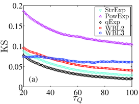
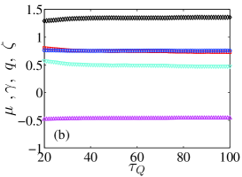
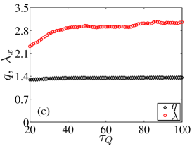
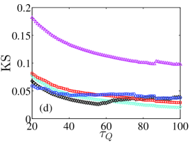
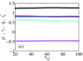
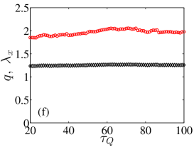
Figure 3: (color online). Plots of fitting results for two stocks. (a-c) Stock 000001. (d-f) Stock 900956. (a, d) Plots of the KS statistics with respect to the mean interval $\tau_{Q}$. The KS statistics is used to describe the agreement between the empirical distribution and the fitting distributions. (b, e) Comparison of the characteristic fitting parameters for the five candidate distributions. (c, f) Plots of the fitting parameters $\lambda_{x}=\tau_{Q}\lambda$ and $q$ with respect to $\tau_{Q}$.

Our goal is to find a distribution that can approximate the distribution of recurrence time. The best candidate distribution will be the one that provides accuracy of fit and ease in estimating the hazard function $W(t|\Delta t)$. Note that the power-law distribution with an exponential cutoff provides the largest body of KS statistics for all the stocks, and that the three-parameter Weibull distribution has fewer KS statistics but requires that too many parameters be estimated. These two distributions are excluded from the candidate list. Because the $q$-exponential distribution has the smallest body of KS statistics for 75.7% of the fits, we use it to capture the distribution of the recurrence intervals. Even when the fits are of bodies of KS statistics that are not the smallest, the $q$-exponential still provides a good approximation of the recurrence time distribution. The $q$-exponential distribution is also highly useful because it allows the derivation of the analytical formula of the hazard function $W(t|\Delta t)$ from the $q$-exponential formula.

4.3 More on distribution parameter behaviors

For each stock and each $\tau_{Q}$ value we fit the corresponding scaled recurrence time $x$ with the $q$-exponential distribution and estimate the distribution parameters $q$ and $\lambda_{x}$. To quantitatively check the scaling behaviors we verify whether the parameters $q$ and $\lambda_{x}$ are independent of $\tau_{Q}$ for the same stock and whether they are the same across different stocks for the same $\tau_{Q}$. For each stock we linearly regress the fitting parameters $q$ and $\lambda_{x}$ with respect to $\tau_{Q}$. Although for $q$ vs $\tau_{Q}$ we find that the maximum absolute slope is 0.006 and the mean slope over all stocks $(5.68\pm 7.77)\times 10^{-4}$, we do not observe comparable small slopes for all stocks when fitting $\lambda_{x}$ vs $\tau_{Q}$. We find 945 stocks with absolute slopes $<0.006$, which is the maximum absolute slope of $q$ vs $\tau_{Q}$. The maximum value of the slope over all stocks is 0.439 and the mean slope $0.0068\pm 0.0213$ for $\lambda_{x}$ vs $\tau_{Q}$. These results suggest that the parameter $q$ is independent of the mean recurrence time $\tau_{Q}$ for all stocks and the parameter $\lambda_{x}$ is independent of $\tau_{q}$ for half of the stocks, which suggests that the scaling behavior in the recurrence intervals for different $\tau_{Q}$ values exists in half of the stocks in the Chinese markets ($945/1891\approx 50\%$).

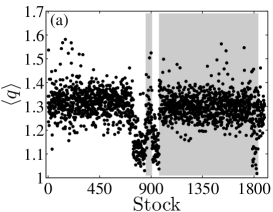
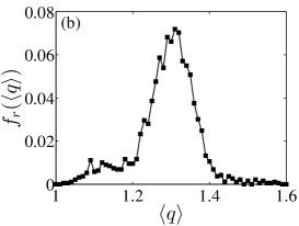
Figure 4: (color online). Plots of the estimated $q$ and $\lambda_{x}$ of $q$-exponential distribution for all stocks. (a) Plots of the fitting parameter $q$ for different stocks. There are five areas, three white areas are separated by two dark areas. For left to right, the first area represents the A-shares in Shenzhen market, the second area is the B-shares in Shenzhen market, the third area stands for ChiNext shares in Shenzhen market, the fourth area corresponds to the A-shares in Shanghai market, and the fifth area is the B-shares in Shanghai market. (b) Frequency of the fitting parameter $q$. (c) Frequency of the fitting parameter $\lambda_{x}$ for different values of $\tau_{Q}$.

Since the value of $q$ does not depend on $\tau_{Q}$, we average the estimated $q$ for different $\tau_{Q}$ values for each stock and plot the mean value of $q$ in Fig. 4(a). Note the three white areas separated by two shadow areas. The five areas from left to right represent A-shares in the Shenzhen market, B-shares in the Shenzhen market, ChiNext shares in the Shenzhen market, A-shares in the Shanghai market, and B-shares in the Shanghai market. Note that there are two groups of stocks, one with a relative smaller value of $\langle q\rangle$ and the other with a much larger value of $\langle q\rangle$. The group of stocks with the smaller $\langle q\rangle$ have been traded in the market less than three years. The panel in Fig. 4(b) shows a plot of the frequency of $\langle q\rangle$ in which there is a significant peak at $\langle q\rangle\approx 1.3$, which corresponds to the average value of $q$ for the stocks in the large $q$ group. Note also that there is a small peak at $q\approx 1.1$, which is the mean value of $q$ for the stocks in the small $q$ group. Because the fitting parameter $\lambda_{x}$ of half of the stocks in our sample depends on $\tau_{Q}$, we plot the frequency of $\lambda_{x}$ of all stocks for different values of $\tau_{Q}$ [see Fig. 4(c)], instead of averaging the $\lambda_{x}$ of different $\tau_{Q}$ for each stock. Note that the distribution curve of $\lambda_{x}$ displays the same pattern across different values of $\tau_{Q}$, the only difference being that the distribution spanning range becomes wider when $\tau_{Q}$ increases. This further indicates that the fitting parameter $\lambda_{x}$ is affected by the mean recurrence time $\tau_{Q}$.

In order to determine whether the $q$-exponential parameters are influenced by market state, i.e., bull or bear, we use a moving window analysis to track the evolution of fitting parameters $q$ and $\lambda_{x}$. Because stocks with trading records shorter than three years have smaller $q$ values, we fix the window size at 48 months and exclude stocks with trading periods shorter than 89 months. We also discard first-month trading data from the stocks remaining because first-month records tend to be partial (i.e., do not span an entire month) and the volatilities for new IPOs excessively large. We arrive at 1395 stocks as subject for our rolling window analysis.

Figure 5: (color online). Plots of the evolution of the estimated $q$ and $\lambda_{x}$ of $q$-exponential distribution for four chosen stocks. From the bottom panel to the up panel, the stock codes are 000001, 200002, 600220, and 900956, respectively. (a) Evolution of $q$. The dash line represents the mean value of $q$ across all windows. The solid line corresponds to the $q$ of the entire period. (b) Evolution of $\lambda_{x}$ for different values of $\tau_{Q}$.

For each stock, we perform the same analysis in each moving window of the series that we perform on the whole series. We first fit the recurrence intervals for different values of $\tau_{Q}$ with the $q$-exponential distribution and estimate the corresponding distribution parameters $q$ and $\lambda_{x}$ in each window. We again find that the parameter $q$ is independent of $\tau_{Q}$ in each window for each stock, but the parameter $\lambda_{x}$ does not exhibit this behavior. We average the $q$ for different values of $\tau_{Q}$ in each window and plot the mean $q$ as a function of the time, which corresponds to the last month of each moving window [see Fig. 5(a)]. For the sake of comparison, the estimated $q$ of the entire period is a solid line and the mean value of $q$ across all the windows is a dashed line. Note that for the four stocks there is a big gap between the solid and dashed line. Note also that the $\langle q\rangle$ curves also exhibit significant fluctuations along the time axis. Figure 5(b) shows the evolution of $\lambda_{x}$ for different values of $\tau_{Q}$. Note that the trajectory of $\lambda_{x}$ exhibits the same trend as the trajectory of $\langle q\rangle$. It is not clear whether these trends reflect stock price tends, but our results demonstrate that the estimated parameters of the $q$-distribution are influenced by market status and thus may be treated as a individual risk factor when explaining market returns.

5 Results of the large volatility prediction

5.1 Hazard probability

The recurrence intervals between volatilities exceeding a threshold $Q$ are well approximated by the $q$-exponential distribution, and that gives us the formula of interval distribution $p(t)=(2-q)\lambda[1+(q-1)\lambda t]^{-\frac{1}{q-1}}$. By substituting this equation into equation (3), we obtain

$$W_{q}(\Delta{t}|t)=1-\left[1+\frac{(q-1)\lambda\Delta t}{1+(q-1)\lambda t}\right]^{1-\frac{1}{q-1}}.$$ (19)

If we designate the top 1% of volatility values (corresponding to the mean recurrence time $\tau_{Q}=100$) to be extreme events, we can estimate the hazard probability $W_{q}(\Delta{t},t)$ in $t$ when fixing $\Delta t$. Figure 6 shows the estimated hazard probability for two stocks when $\Delta t=1$, 5, and 10. Note that both the solid lines indicating the analytical solution equation (19) and the markers indicating the empirical data decrease slowly and in each panel are in good agreement. The decreasing trend of $W(\Delta t|t)$ is consistent with the clustering behavior in the volatility series. Note that the hazard probability $W(\Delta t|t)$ is universal and can be used to estimate the risk in any kind of time series.

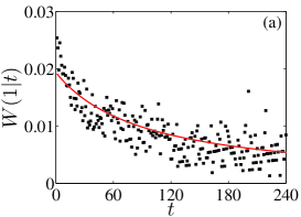
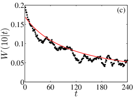
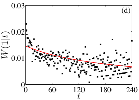
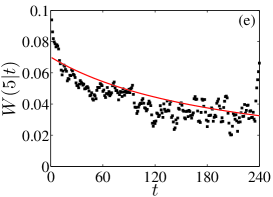
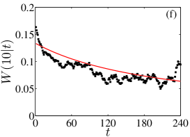
Figure 6: (color online). Plot of hazard probability $W(\Delta t|t)$ for two stocks and $\Delta t=1$, $5$, and $10$. (a-c) Stock 000001. (d-f) Stock 900956.

5.2 Predicting large volatilities

To forecase large volatility events in a volatililty series we first calculate the recurrence time for a given $\tau_{Q}$, e.g., $\tau_{Q}=100$, and estimate the distribution of parameters. The hazard probability $W(1|t)$ that an extreme event will occur in the next period is determined using equation (19) and the estimated distribution parameters. Once the hazard probability breaks though the predefined threshold $Q_{p}$, an alarm will be triggered, warning that a large volatility event is immanent. Figure 7(a) plots a subseries of the volatility values and highlights events above threshold $Q$ in the top panel, which correspond to the mean recurrence time $\tau_{Q}$. The risk probability $W(1|t)$ is shown in the bottom panel. Note that $W(1|t)$ decreases as time $t$ elapsed from the last large volatility event increases. Threshold $Q_{p}$ is plotted as a horizontal line to show the activating alarm process. By varying $Q_{p}$ within a $[0,1]$ range, we obtain all pairs of $(A,D)$.

Figure 7(b) shows the ROC curves for ten stocks. Note that all ten curves are above the dashed line $D=A$, indicating that our prediction is not random. The ten curves do not overlap, indicating that the accuracy of this prediction algorithm varies for different stocks. For the same false alarm $A$ (where a vertical dashed line is plotted at $A=0.1$ as an example), stock 900901 has the highest correct prediction rate and stock 300066 the lowest. We also calculate the correct prediction rate $D_{A=0.1}$ for all stocks at the false alarm level of 0.1. Figure 7(c) shows the frequency plots of $D_{A={\rm{0.1}}}$. Note that the peak is centered at $\approx 0.2$, 10% higher than a random prediction. We also find there are nine stocks with $D_{A=0.1}>0.4$. The top three values are 0.7, 0.68, and 0.60 for stocks 000529, 000557, and 000592, indicating that our forecasting algorithm can accurately predict the large volatilities of these three stocks. Previous research has indicated that the efficiency of the algorithm is primarily influenced by the linear and nonlinear memory behavior in the original volatilities [4]. Our results here indicate that the behavior of stocks with stronger memory behaviors, such as volatility clustering and multifactality, could be more accurately predicted using our algorithm. Our algorithm only takes into consideration the probability distribution of recurrence intervals, but if the memory behavior of recurrence intervals were also included we believe that its predictive accuracy would be greatly inhanced.

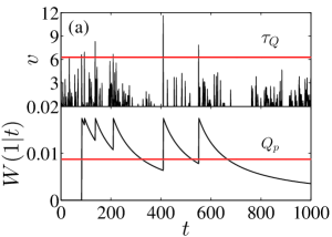
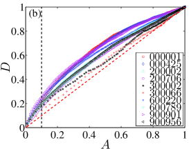
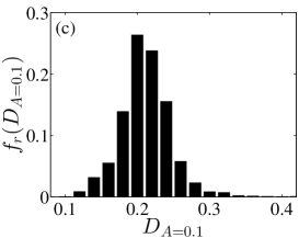
Figure 7: (color online). Prediction of large volatilities. (a) Plots of a representative volatility series in the top panels and hazard probability $W(1|\Delta t)$ in the bottom panels. (b) Plots of ROC curves for ten stocks. (c) Distribution plots of the correct prediction rates at the false alarm level of 0.1 for all stocks.

6 Conclusion

In this work, we have utilized a decision-making algorithm to forecast the occurrence of large volatilities in Chinese stock markets based on the hazard probability, which is derived from the distribution of recurrence intervals between the volatilities exceeding a threshold $Q$. By fitting the volatility recurrence intervals by means of five candidate distributions and comparing their KS statistics, we have found that the volatility recurrence intervals are well approximated by the $q$-exponential distribution. The fitting parameter $q$ is found to be independent of the mean recurrence time $\tau_{q}$, which is at a one-to-one correspondence with the threshold $Q$, for all the stocks in our sample. However the parameter $\lambda_{x}$ of the $q$-distribution does not exhibit the same behavior as $q$. For half of the stocks, $\lambda_{x}$ exhibits a strong dependence on $\tau_{Q}$. Using a moving window analysis, we have found that both parameters are influenced by market status and exhibit the same trend with the evolution of time. This behavior may have potential applications for explaining stock return volitility.

Using the $q$-distribution formula, we have derived an analytical solution of the hazard probability $W(\Delta t|t)$ of the next large volatility event above the threshold $Q$ within a short time interval $\Delta t$ after an elapsed time $t$ from the last large volatility above $Q$. This analytical solution $W(\Delta t|t)$ is in good agreement with the empirical risk probability derived from real stock data. We have adopted a decision-marking algorithm and have used the hazard probability to forecast large volatilities. At the false alarm level of 0.1, we have found that the average correct predicting rate is 0.2 for all stocks. We have also found that there are three stocks with a correct predicting rate is greater than 0.6, indicating that our predicting algorithm is accurate in forecasting the large volatilities. Our findings may shed new light on our understanding of extreme volatility behavior and may have potential applications in managing stock market risk.

Appendix A Maximum likelihood estimation of distribution parameters

A.1 Stretched exponential distribution

To estimate the parameters of Eq. (14), the first step is to use $\int_{0}^{\infty}f(x)=1$ and $\int_{0}^{\infty}xf(x)=1$ to reduce the number of parameters.For the first integral, we have

$$\int_{0}^{\infty}f(x){\rm{d}}{x}=\int_{0}^{\infty}a\tau_{Q}e^{-(b\tau_{Q}x)^{\mu}}{\rm{d}}{x}=1,$$ (20)

Let $y=(b\tau_{Q}x)^{\mu}$, we have $x=\frac{y^{1/\mu}}{b\tau_{Q}}$ and ${\rm{d}}x=\frac{y^{1/\mu-1}{\rm{d}}y}{\mu b\tau_{Q}}$. Then, we can obtain

$$\int_{0}^{\infty}a\tau_{Q}e^{-(b\tau_{Q}x)^{\mu}}{\rm{d}}{x}=\int_{0}^{\infty}a\tau_{Q}e^{-y}\frac{y^{1/\mu-1}}{\mu b\tau_{Q}}{\rm{d}}y=\frac{a}{\mu b}\int_{0}^{\infty}y^{1/\mu-1}e^{-y}{\rm{d}}y=\frac{a}{\mu b}\Gamma(\frac{1}{\mu})=1.$$ (21)

For the second integral, we have

$$\int_{0}^{\infty}xf(x){\rm{d}}{x}=\int_{0}^{\infty}xa\tau_{Q}e^{-(b\tau_{Q}x)^{\mu}}{\rm{d}}{x}=1,$$ (22)

Again, we let $y=(b\tau_{Q}x)^{\mu}$, we have $x=\frac{y^{1/\mu}}{b\tau_{Q}}$ and ${\rm{d}}x=\frac{y^{1/\mu-1}{\rm{d}}y}{\mu b\tau_{Q}}$. Then, we can obtain

$$\int_{0}^{\infty}ax\tau_{Q}e^{-(b\tau_{Q}x)^{\mu}}{\rm{d}}{x}=\int_{0}^{\infty}\frac{y^{1/\mu}}{b\tau_{Q}}a\tau_{Q}e^{-y}\frac{y^{1/\mu-1}}{\mu b\tau_{Q}}{\rm{d}}y=\frac{a}{\mu b^{2}\tau_{Q}}\int_{0}^{\infty}y^{2/\mu-1}e^{-y}{\rm{d}}y=\frac{a}{\mu b^{2}\tau_{Q}}\Gamma(\frac{2}{\mu})=1.$$ (23)

Through solving the equations, the parameters $a$ and $b$ could be formulated by the exponent $\mu$ and $\tau_{Q}$,

$$a=\frac{\mu\Gamma(2/\mu)}{\Gamma(1/\mu)^{2}\tau_{Q}},~{}~{}b=\frac{\Gamma(2/\mu)}{\Gamma(1/\mu)\tau_{Q}}$$ (24)

The likelihood function of the stretched exponential distribution can be written as

$$L=\prod_{i}^{n}a\tau_{Q}\exp[-(b\tau_{Q}x_{i})^{\mu}],$$ (25)

Taking logarithm on both side, we have

$$\ln L=n\ln a+n\ln\tau_{Q}-\sum_{i}^{n}(b\tau_{Q}x_{i})^{\mu},$$ (26)

By submitting Eq. (24) into Eq. (26), the log likelihood function of the stretched exponential distribution has only one variable $\mu$. Our purpose is to find the value of $\mu$ which is associated with the maximum value of the $\ln L$. Here, it is very hard to obtain the expression by taking a derivative of $\ln L$ with respect to $\mu$. Hence, we just estimate the function value of $\ln L$ by changing $\mu$ from 0 to 5 with a step of $10^{-6}$. We locate the $\mu$ with the maximum $\ln L$ as the solution of our maximum likelihood estimation.

A.2 Power-law distribution with an exponential cutoff

As the same way as the stretched exponential, we use $\int_{0}^{\infty}f(x)=1$ and $\int_{0}^{\infty}xf(x)=1$ to reduce the number of parameters. For the first integral, we have

$$\int_{0}^{\infty}f(x){\rm{d}}x=\int_{0}^{\infty}c\tau_{Q}^{-\gamma}x^{-\gamma-1}e^{-k\tau_{Q}x}{\rm{d}}x=1,$$ (27)

Let $y=k\tau_{Q}x$, we have $x=\frac{y}{k\tau_{Q}}$ and ${\rm{d}}x=\frac{{\rm{d}}y}{k\tau_{Q}}$. Then, we obtain

$$\int_{0}^{\infty}c\tau_{Q}^{-\gamma}x^{-\gamma-1}e^{-k\tau_{Q}x}{\rm{d}}x=\int_{0}^{\infty}c\tau_{Q}^{-\gamma}\left(\frac{y}{k\tau_{Q}}\right)^{-\gamma-1}e^{-y}\frac{{\rm{d}}y}{k\tau_{Q}}=\frac{c}{k^{-\gamma}}\int_{0}^{\infty}y^{-\gamma-1}e^{-y}=\frac{c}{k^{-\gamma}}\Gamma(-\gamma)=1.$$ (28)

For the second integral, we have

$$\int_{0}^{\infty}xf(x){\rm{d}}x=\int_{0}^{\infty}xc\tau_{Q}^{-\gamma}x^{-\gamma-1}e^{-k\tau_{Q}x}{\rm{d}}x=1,$$ (29)

Again, we let $y=k\tau_{Q}x$, we have $x=\frac{y}{k\tau_{Q}}$ and ${\rm{d}}x=\frac{{\rm{d}}y}{k\tau_{Q}}$. Then, we obtain

$$\int_{0}^{\infty}xc\tau_{Q}^{-\gamma}x^{-\gamma-1}e^{-k\tau_{Q}x}{\rm{d}}x=\int_{0}^{\infty}c\frac{y}{k\tau_{Q}}\tau_{Q}^{-\gamma}\left(\frac{y}{k\tau_{Q}}\right)^{-\gamma-1}e^{-y}\frac{{\rm{d}}y}{k\tau_{Q}}=\frac{c}{k^{1-\gamma}\tau_{Q}}\int_{0}^{\infty}y^{(1-\gamma)-1}e^{-y}=\frac{c}{k^{1-\gamma}\tau_{Q}}\Gamma(1-\gamma)=1.$$ (30)

Through solving the two equations, we obtain that

$$k=\frac{\Gamma(1-\gamma)}{\Gamma(-\gamma)\tau_{Q}}=\frac{-\gamma}{\tau_{Q}},~{}~{}b=\left(\frac{-\gamma}{\tau_{Q}}\right)^{-\gamma}\frac{1}{\Gamma(-\gamma)}$$ (31)

The likelihood function of the power-law distribution with an exponential cutoff can be written as

$$L=\prod_{i}^{n}c\tau_{Q}^{-\gamma}x^{-\gamma-1}e^{-k\tau_{Q}x},$$ (32)

Taking logarithm on both side, we have

$$\ln L=n\ln c-\gamma n\ln\tau_{Q}-(\gamma+1)\sum_{i}^{n}\ln x_{i}-\sum_{i}^{n}k\tau_{Q}x_{i},$$ (33)

By submitting Eq. (31) into Eq. (33), the log likelihood function of the power-law distribution with an exponential distribution has only one variable $\gamma$. Our purpose is to find the value of $\gamma$ which is associated with the maximum value of the $\ln L$. Here, it is very hard to obtain the expression by taking a derivative of $\ln L$ with respect to $\gamma$. Hence, we just estimate the function value of $\ln L$ by changing $\mu$ from -1 to 0 with a step of $10^{-6}$. We locate the $\gamma$ with the maximum $\ln L$ as the solution of our maximum likelihood estimation.

References

- [1] S. Hallerberg, E. G. Altmann, D. Holstein, H. Kantz, Precursors of extreme increments, Phys. Rev. E 75 (2007) 016706. doi:10.1103/PhysRevE.75.016706.
- [2] S. Hallerberg, H. Kantz, Influence of the event magnitude on the predictability of an extreme event, Phys. Rev. E 77 (2008) 011108. doi:10.1103/PhysRevE.77.011108.
- [3] M. I. Bogachev, A. Bunde, Improved risk estimation in multifractal records: Application to the value at risk in finance, Phys. Rev. E 80 (2009) 026131. doi:10.1103/PhysRevE.80.026131.
- [4] M. I. Bogachev, A. Bunde, On the predictability of extreme events in records with linear and nonlinear long-range memory: Efficiency and noise robustness, Physica A 390 (2011) 2240–2250. doi:10.1016/j.physa.2011.02.024.
- [5] A. Bunde, J. F. Eichner, S. Havlin, J. W. Kantelhardt, Return intervals of rare events in records with long-term persistence, Physica A 342 (2004) 308–314.
- [6] A. Bunde, J. F. Eichner, J. W. Kantelhardt, S. Havlin, Long-term memory: A natural mechanism for the clustering of extreme events and anomalous residual times in climate records, Phys. Rev. Lett. 94 (2005) 048701. doi:10.1103/PhysRevLett.94.048701.
- [7] A. Saichev, D. Sornette, “Universal” distribution of interearthquake times explained, Phys. Rev. Lett. 97 (2006) 078501. doi:10.1103/PhysRevLett.97.078501.
- [8] C. Liu, Z.-Q. Jiang, F. Ren, W.-X. Zhou, Scaling and memory in the return intervals of energy dissipation rate in three-dimensional fully developed turbulence, Phys. Rev. E 80 (2009) 046304.
- [9] M. I. Bogachev, I. S. Kireenkov, E. M. Nifontov, A. Bunde, Statistics of return intervals between long heartbeat intervals and their usability for online prediction of disorders, New J. Phys. 11 (2009) 063036. doi:10.1088/1367-2630/11/6/063036.
- [10] M. I. Bogachev, A. Bunde, Universality in the precipitation and river runoff, EPL (Europhys. Lett.) 97 (2012) 48011. doi:10.1209/0295-5075/97/48011.
- [11] M. I. Bogachev, A. Bunde, On the occurrence and predictability of overloads in telecommunication networks, EPL (Europhys. Lett.) 86 (2009) 66002. doi:10.1209/0295-5075/86/66002.
- [12] S.-M. Cai, Z.-Q. Fu, T. Zhou, J. Gu, P.-L. Zhou, Scaling and memory in recurrence intervals of Internet traffic, EPL (Europhys. Lett.) 87 (4) (2009) 68001. doi:10.1209/0295-5075/87/68001.
- [13] K. Yamasaki, L. Muchnik, S. Havlin, A. Bunde, H. E. Stanley, Scaling and memory in volatility return intervals in financial markets, Proc. Natl. Acad. Sci. U.S.A. 102 (2005) 9424–9428. doi:10.1073/pnas.0502613102.
- [14] W.-J. Xie, Z.-Q. Jiang, W.-X. Zhou, Extreme value statistics and recurrence intervals of NYMEX energy futures volatility, Econ. Model. 36 (2014) 8–17. doi:10.1016/j.econmod.2013.09.011.
- [15] K. Yamasaki, L. Muchnik, S. Havlin, A. Bunde, H. E. Stanley, Scaling and memory in return loss intervals: Application to risk estimation, in: H. Takayasu (Ed.), Practical Fruits of Econophysics, Springer-Verlag, Berlin, 2006, pp. 43–51.
- [16] M. I. Bogachev, J. F. Eichner, A. Bunde, Effect of nonlinear correlations on the statistics of return intervals in multifractal data sets, Phys. Rev. Lett. 99 (2007) 240601. doi:10.1103/PhysRevLett.99.240601.
- [17] M. I. Bogachev, A. Bunde, Memory effects in the statistics of interoccurrence times between large returns in financial record, Phys. Rev. E 78 (2008) 036114. doi:10.1103/PhysRevE.78.036114.
- [18] F. Ren, W.-X. Zhou, Recurrence interval analysis of high-frequency financial returns and its application to risk estimation, New J. Phys. 12 (2010) 075030. doi:10.1088/1367-2630/12/7/075030.
- [19] J. Ludescher, C. Tsallis, A. Bunde, Universal behaviour of interoccurrence times between losses in financial markets: An analytical description, EPL (Europhys. Lett.) 95 (2011) 68002. doi:10.1209/0295-5075/95/68002.
- [20] L.-Y. He, S.-P. Chen, A new approach to quantify power-law cross-correlation and its application to crude oil markets, Physica A 390 (2011) 3806–3814. doi:10.1016/j.physa.2011.06.013.
- [21] H. Meng, F. Ren, G.-F. Gu, X. Xiong, Y.-J. Zhang, W.-X. Zhou, W. Zhang, Effects of long memory in the order submission process on the properties of recurrence intervals of large price fluctuations, EPL (Europhys. Lett.) 98 (5) (2012) 38003. doi:10.1209/0295-5075/98/38003.
- [22] Y.-Y. Suo, D.-H. Wang, S.-P. Li, Risk estimation of csi 300 index spot and futures in china from a new perspective, Econometrica 49 (2015) 344–353. doi:10.1016/j.econmod.2015.05.011.
- [23] B. Podobnik, D. Horvatic, A. M. Petersen, H. E. Stanley, Cross-correlations between volume change and price change, Proc. Natl. Acad. Sci. U.S.A. 106 (2009) 22079–22084. doi:10.1073/pnas.0911983106.
- [24] F. Ren, W.-X. Zhou, Recurrence interval analysis of trading volumes, Phys. Rev. E 81 (2010) 066107. doi:10.1103/PhysRevE.81.066107.
- [25] W. Li, F.-Z. Wang, S. Havlin, H. E. Stanley, Financial factor influence on scaling and memory of trading volume in stock market, Phys. Rev. E 84 (2011) 046112. doi:10.1103/PhysRevE.84.046112.
- [26] T. Kaizoji, M. Kaizoji, Power law for the calm-time interval of price changes, Physica A 336 (2004) 563–570. doi:10.1016/j.physa.2003.12.054.
- [27] J. W. Lee, K. E. Lee, P. A. Rikvold, Waiting-time distribution for Korean stock-market index KOSPI, J. Korean Phys. Soc. 48 (2006) S123–S126.
- [28] A. Greco, L. Sorriso-Valvo, V. Carbone, S. Cidone, Waiting time distributions of the volatility in the Italian MIB30 index: Clustering or Poisson functions?, Physica A 387 (2008) 4272–4284. doi:10.1016/j.physa.2008.03.007.
- [29] F.-Z. Wang, K. Yamasaki, S. Havlin, H. E. Stanley, Scaling and memory of intraday volatility return intervals in stock markets, Phys. Rev. E 73 (2006) 026117. doi:10.1103/PhysRevE.73.026117.
- [30] F. Wang, P. Weber, K. Yamasaki, S. Havlin, H. E. Stanley, Statistical regularities in the return intervals of volatility, Eur. Phys. J. B 55 (2007) 123–133. doi:10.1140/epjb/e2006-00356-9.
- [31] W.-S. Jung, F.-Z. Wang, S. Havlin, T. Kaizoji, H. T. Moon, H. E. Stanley, Volatility return intervals analysis of the Japanese market, Eur. Phys. J. B 62 (2008) 113–119. doi:10.1140/epjb/e2008-00123-0.
- [32] T. Qiu, L. Guo, G. Chen, Scaling and memory effect in volatility return interval of the Chinese stock market, Physica A 387 (2008) 6812–6818. doi:10.1016/j.physa.2008.09.002.
- [33] F. Ren, G.-F. Gu, W.-X. Zhou, Scaling and memory in the return intervals of realized volatility, Physica A 388 (2009) 4787–4796. doi:10.1016/j.physa.2009.08.009.
- [34] F. Ren, L. Guo, W.-X. Zhou, Statistical properties of volatility return intervals of Chinese stocks, Physica A 388 (2009) 881–890. doi:10.1016/j.physa.2008.12.005.
- [35] W. Jeon, H.-T. Moon, G. Oh, J.-S. Yang, W.-S. Jung, Return intervals analysis of the Korean stock market, J. Korean Phys. Soc. 56 (2010) 922–925. doi:10.3938/jkps.56.922.
- [36] F. Wang, J. Wang, Statistical analysis and forecasting of return interval for SSE and model by lattice percolation system and neural network, Comput. Ind. Eng. 62 (2012) 198–205. doi:10.1016/j.cie.2011.09.007.
- [37] J. Ludescher, A. Bunde, Universal behavior of the interoccurrence times between losses in financial markets: Independence of the time resolution, Phys. Rev. E 90 (2014) 062809. doi:10.1103/PhysRevE.90.062809.
- [38] D. Sornette, L. Knopoff, The paradox of the expected time until the next earthquake, Bull. Seism. Soc. Am. 87 (1997) 789–798.
- [39] B. Bollen, B. Inder, Estimating daily volatility in financial markets utilizing intraday data, J. Emp. Finance 9 (2002) 551–562. doi:10.1016/S0927-5398(02)00010-5.
- [40] M. Politi, E. Scalas, Fitting the empirical distribution of intertrade durations, Physica A 387 (2008) 2025–2034. doi:10.1016/j.physa.2007.11.018.
- [41] Z.-Q. Jiang, W. Chen, W.-X. Zhou, Scaling in the distribution of intertrade durations of Chinese stocks, Physica A 387 (2008) 5818–5825. doi:10.1016/j.physa.2008.06.039.