Lifetime Maximization of Wireless Sensor Networks with a Mobile Source Node

Abstract

We study the problem of routing in sensor networks where the goal is to maximize the network’s lifetime. Previous work has considered this problem for fixed-topology networks. Here, we add mobility to the source node, which requires a new definition of the network lifetime. In particular, we redefine lifetime to be the time until the source node depletes its energy. When the mobile node’s trajectory is unknown in advance, we formulate three versions of an optimal control problem aiming at this lifetime maximization. We show that in all cases, the solution can be reduced to a sequence of Non-Linear Programming (NLP) problems solved on line as the source node trajectory evolves and include simulation examples to illustrate our results. When the mobile node’s trajectory is known in advance, we formulate an optimal control problem which, in this case, requires an explicit off-line numerical solution.

I Introduction

A Wireless Sensor Network (WSN) is a spatially distributed wireless network consisting of low-cost autonomous nodes which are mainly battery powered and have sensing and wireless communication capabilities [1]. Applications range from exploration, surveillance, and target tracking, to environmental monitoring (e.g., pollution prevention, agriculture). Power management is a key issue in WSNs, since it directly impacts their performance and their lifetime in the likely absence of human intervention for most applications of interest. Since the majority of power consumption is due to the radio component [2], nodes usually rely on short-range communication and form a multi-hop network to deliver information to a base station. Routing schemes in WSNs aim to deliver data from the data sources (nodes with sensing capabilities) to a data sink (typically, a base station) in an energy-efficient and reliable way. The problem of routing in WSNs with the goal of optimizing performance metrics that reflect the limited energy resources of the network has been widely studied for static (i.e., fixed topology) networks [3],[4],[5],[6],[7]. In recent years, mobility in WSNs has been increasingly introduced and studied [8],[9] and [10] with the aim of enhancing their capabilities. In fact, as discussed in [11], mobility can affect different aspects of WSN design, including connectivity, cost, reliability and energy efficiency. There are various ways to exploit WSN mobility and incorporating it into different network components. For instance, in [9] sink mobility is exploited and a Linear Programming (LP) formulation is proposed for maximizing the network lifetime by finding the optimal sink node movement and sojourn time at different nodes in the network. In [10] mobile nodes (mules) are used to deliver data to the base station. WSNs with partial mobility are studied in [12]. As discussed in [13], there exist two modes for sensor nodes mobility: weak mobility, forced by the death of some sensor nodes and strong mobility using an external agent [14],[15].

In this paper, we focus on the lifetime maximization problem in WSNs when source nodes are mobile. This situation frequently arises when a mobile sensor node is used to track one or more mobile targets or when there is a large area to be monitored that far exceeds the range of one or more static sensors. In the case of a fully static network the lifetime maximization problem was studied in [5] and [6] by defining the WSN lifetime as the time until the first node depletes its energy. Since it is often the case that an optimal policy controlling a static WSN’s resources leads to individual node lifetimes being the same or almost the same as those of others, this definition is a good characterization of the overall network’s lifetime in practice. In [5] routing was formulated as an optimal control problem with controllable routing probabilities over network links and it was shown that in a fixed network topology there exists an optimal policy consisting of time-invariant routing probabilities. Moreover, the optimal control problem may be converted into the LP formulation used in [6]. It is worth mentioning that a routing policy based on probabilities can easily be implemented by transforming these probabilities to packet flows over links and using simple mechanisms to ensure that flows are maintained over time. In [16] the simplifying assumption of idealized batteries used as energy sources for nodes was also relaxed and a more elaborate model was used to capture nonlinear dynamic phenomena that are known to occur in non-ideal batteries. A somewhat surprising result was that again an optimal policy exists which consists of time-invariant routing probabilities and that in fact this property is independent of the parameters of the battery model. However, this attractive property for routing is limited to a fixed network topology.

Adding mobility to nodes raises several questions. First, one can no longer expect that a routing policy would be time invariant. Second, it is no longer reasonable to define the WSN lifetime in terms of the the first node depleting its energy. For instance, if a source node travels far from some relay nodes it was originally using, it is likely that it should no longer rely on them for delivering data to the base station. In this scenario, the network remains “alive” even when these nodes die. Thus, in view of node mobility, we need to revisit the definition of network lifetime. Finally, if a routing policy is time-varying, then it has to be re-evaluated sufficiently fast to accommodate the real-time operation of a WSN.

In the sequel, we consider mobility added to the source node and assume that any such node travels along a trajectory that it determines and which may or may not be known in advance. We limit ourselves to a single source node (the case of multiple mobile source nodes depends on the exact setting and is not addressed in this paper). While on its trajectory, the source node continuously performs sensing tasks and generates data. Our goal is to derive an optimal routing scheme in order to maximize the network lifetime, appropriately redefined to focus on the mobile source node. Assuming first that the source node trajectory is not known in advance, we formulate three optimal control problems with differences in their terminal costs and terminal constraints and investigate how they compare in terms of the optimal routing policy obtained, total energy consumption, and the actual network lifetime. We will also limit ourselves to ideal battery dynamics for all nodes. However, adopting non-ideal battery models as in [16] does not change our analysis and only complicates the solution computation. We then consider the more challenging (from a computational perspective) problem where the source node’s trajectory is known in advance, in which case this information can be incorporated into an optimal lifetime maximization policy.

In Section II, we define the network model and the energy consumption model is presented in Section III. In Section IV we formulate the maximum lifetime optimization problem for a WSN with a mobile source node whose trajectory is not known in advance. Starting with a new definition for the network lifetime, we show that the solution is a sequence of Non-Linear Programming (NLP) problems along the source node trajectory. Numerical examples are included to illustrate our analytical results. In Section V, we consider the case when the source node trajectory is known in advance and show that its solution leads to a Two Point Boundary Value Problem (TPBVP).

II Network model

Consider a network with $N+1$ nodes where $0$ and $N$ denote the source and destination (base station) nodes respectively. Nodes $1,...,N-1$ act as relay nodes to deliver data packets from the source node to the base station. We assume the source node is mobile and travels along a trajectory with a constant velocity while generating data packets which need to be transferred to the fixed base through static relay nodes. First, we assume the trajectory is not known in advance. Then, we discuss the case when the trajectory is known in Section V. Except for the base station whose energy supply is not constrained, a limited amount of energy is available to all other nodes. Let $r_{i}(t)$ be the residual energy of node $i$, $i=0,\ldots,N-1$, at time $t$. The dynamics of $r_{i}(t)$ depend on the battery model used at node $i$. Here, we assume ideal battery dynamics in which energy is depleted linearly with respect to the node’s load, $I_{i}(t)$, i.e.,

$$\dot{r}_{i}(t)=-I(t)$$ (1)

The distance between nodes $i$ and $j$ at time $t$ is denoted by $d_{i,j}(t)$. Since the source node is mobile, $d_{0,j}(t)$ is time-varying for all $j=1,...,N-1$. However, $d_{i,j}(t)=d_{i,j},\ i=1,...,N-1,\ j=2,...,N$ are treated as time-invariant with the assumption that the source node cannot be used as a relay, i.e., any node $i>0$ must transfer data to other relay nodes $j>0$, $j\neq i$ or directly to the base station node $N$. The source node can send data packets to any of the relay nodes as well as to the base station, while relay nodes can transmit/receive data packets to/from nodes in their transmission range. Let $O(i)$ and $I(i)$ denote the set of nodes to/from which node $i$ can send/receive data packets respectively. Then, $O(i)=\left\{j:d_{i,j}\leq\tau_{i}\right\}$ and $I(i)=\{j:d_{j,i}\leq\tau_{j}\}$ where $\tau_{i},\ i=1,...,N-1$ denotes the transmission range of node $i$. We define $w_{ij}(t)$ to be the routing probability of a packet from node $i$ to node $j$ at time $t$ (equivalently, a data flow from $i$ to $j$) and the vector $w(t)=[w_{ij}(t)]^{\prime}$ defines the control in our problem. Let us also define $\mathbf{r}(t)=[r_{0}(t),...,r_{N-1}(t)]$ as the vector of residual energies at time $t$. For simplicity, the data sending rate of source node $0$ is normalized to $1$ and let $G_{i}(w)$ denote the data packet inflow rate to node $i$. Given these definitions, we can express $G_{i}(w)$ through the following flow conservation equations:

$$G_{i}(w) ={\displaystyle\sum\limits_{k\in I(i)}}w_{ki}(t)G_{k}(w),\text{\ }i=1,\ldots,N,\ G_{0}(w)=1$$ (2)

III Energy Consumption Model

In our WSN environment, the battery workload $I(t)$ is due to three factors: the energy needed to sense a bit, $E_{sense}$, the energy needed to receive a bit, $E_{rx}$, and the energy needed to transmit a bit, $E_{tx}$. If the distance between two nodes is $d$, we have: $E_{tx}=p(d),\text{ \ }E_{rx}=C_{r},\text{ \ }E_{sense}=C_{e}$, where $C_{r}$, $C_{e}$ are given constants dependent on the communication and sensing characteristics of nodes, and $p(d)\geq 0$ is a function monotonically increasing in $d$; the most common such function is $p(d)=C_{f}+C_{s}d^{\beta}$ where $C_{f}$, $C_{s}$ are given constants and $\beta$ is a constant dependent on the medium involved. We will use the common situation where $\beta=2$ in the rest of the paper, but this has no effect on our approach. We shall use this  energy model, but ignore the sensing energy $C_{e}$, i.e., set $C_{e}=0$ (otherwise, $C_{e}$ is simply added to the source node’s workload without affecting the analysis). Clearly, this is a relatively simple energy model that does not take into consideration the channel quality or the Shannon capacity of each wireless channel. The ensuing optimal control analysis is not critically dependent on the exact form of the energy consumption model attributed to communication, although the ultimate optimal value of $w(t)$ obviously is. For any node $i=1,\ldots,N-1$, the workload $I_{i}(t)$ at that node is given by

$$I_{i}(w(t))=G_{i}(w(t))[\sum_{j\in O(i)}w_{ij}(t)(C_{s}d_{i,j}^{\beta}(t)+C_{f})+C_{r}]$$ (3)

and the workload $I_{0}(t)$ at the source node $0$ (recalling that $G_{0}(w(t))=1$) is given by

$$I_{0}(w(t))=\sum_{j\in O(0)}w_{0j}(t)(C_{s}d_{0,j}^{\beta}(t)+C_{f})$$ (4)

Assuming an ideal battery behavior for all nodes as in (1), the state variables for our problem are $r_{i}(t),\ i=0,...,N-1$. Note that $d_{0,j}(t)=\|(x_{0}(t),y_{0}(t))-(x_{j},y_{j})\|$, the Euclidean distance of the source node from any other node is known at any time instant $t$ (but not in advance) as determined by the source node’s trajectory. Finally, observe that by controlling the routing probabilities $w_{ij}(t)$ in (4) and (3) we directly control node $i$’s battery discharge process.

IV Optimal control problem formulation

Our objective is to maximize the WSN lifetime by controlling the routing probabilities $w_{ij}(t)$. For a static network, where all nodes including the source node are fixed, the network lifetime is usually defined as the time until the first node depletes its battery [16], [6]. However, when the source node is mobile, this definition of network lifetime is no longer appropriate as explained in Section I. In the sequel, we formulate three optimal control problems for maximizing lifetime in a WSN with a mobile source node and investigate their relative effect in terms of an optimal routing policy, total energy consumption, and the network lifetime.

IV-A Optimal Control Problem - I

We define the network lifetime as the time when the source node runs out of energy. Consider a fixed time $t$ when the source node is at position $(x_{0}(t),y_{0}(t))\in\mathbb{R}^{2}$. In the absence of any future information regarding the position of this node (e.g., the node may actually stop for some time interval before moving again), the routing problem we face is one of a fixed topology WSN similar to the one in [16] but with different terminal state constraints due to the new network lifetime definition. Thus, this maximum lifetime optimal control problem is formulated as follows, using the variables defined in (2), (3) and (4):

$$\min_{w(t)}-\int_{0}^{T}dt$$ (5)

$$\text{s.t.\ \ }\dot{r}_{i}(t)=-I_{i}(w(t)),\ r_{i}(0)=R_{i},\quad i=0,..,N-1$$ (6)

$$I_{i}(w(t))=G_{i}(w(t))[\sum_{j\in O(i)}w_{ij}(t)(C_{s}d_{i,j}^{2}+C_{f})+C_{r}],$$

$$\quad\quad i=1,...,N-1$$ (7)

$$I_{0}(w(t))=\sum_{j\in O(0)}w_{0j}(t)(C_{s}d_{0,j}^{2}(t)+C_{f})$$ (8)

$$d_{0,j}(t)=\|(x_{0}(t),y_{0}(t))-(x_{j},y_{j})\|,\ x_{0}(t),y_{0}(t)\text{ given}$$

$$G_{i}(w(t))={\displaystyle\sum\limits_{k\in I(i)}}w_{ki}(t)G_{k}(w(t)),\text{ }i=1,..,N-1$$ (9)

$$\sum_{j\in O_{i}}w_{ij}(t)=1,\quad 0\leq w_{ij}(t)\leq 1,\text{ }i=0,\ldots,N-1$$ (10)

$$r_{0}(T)=0$$ (11)

$$r_{0}(t)>0,\ t\in[0,T);\text{ }r_{i}(t)\geq 0,\text{ }i=1,..,N-1,\text{ }t\in[0,T]$$ (12)

where $r_{i}(t)$, $i=0,...,N-1$, are the state variables representing the node $i$ battery dynamics and $(x_{0}(t),y_{0}(t))$ are the given instantaneous coordinates of the source node at time $t$. Control constraints are specified through (10). Finally, (11) provides the boundary conditions for $r_{0}(t)$ at $t=T$ requiring that the terminal time is the time when the source node depletes its energy. In what follows, we will use $w^{\ast}(t)$ to denote the optimal routing vector at the fixed time $t$.

IV-A1 Optimal control problem I solution

We begin with the Hamiltonian for this optimal control problem:

$$H(\mathbf{r},x_{0},y_{0},w,\lambda,t)= -1+\lambda_{0}(t)(-I_{0}(t))+$$

$$\sum_{i=1}^{N-1}\lambda_{i}(t)(-I_{i}(t))$$ (13)

where $\lambda_{i}(t)$ is the costate corresponding to $r_{i}(t),\ i=0,...,N-1$ and must satisfy:

$$\dot{\lambda}_{i}(t)=-\dfrac{\partial H}{\partial r_{i}}=0\quad i=0,...,N-1$$ (14)

Therefore, $\lambda_{i}$, $i=0,...,N-1$, are constants. To determine their values we make use of the boundary conditions which follow from (11), i.e., the terminal state constraint function is $\Phi(\mathbf{r}(T))=\nu r_{0}(T)$ and the costate boundary conditions are given by:

$$\lambda_{i}(T)=\dfrac{\partial\Phi(r_{0}(T),...,r_{N-1}(T))}{\partial r_{i}(T)},\quad i=0,...,N-1$$

which implies that

$$\lambda_{i}=0\quad i=1,...,N-1,\quad\lambda_{0}=\nu$$ (15)

where $\nu$ is some scalar constant. Finally, the optimal solution must satisfy the transversality condition $H(T)+\left.{\partial\Phi}/{\partial t}\right|_{t=T}=0$, i.e., $-1+\nu\dot{r}_{0}(T)+\nu\dot{r}_{0}(T)=0$, which yields: $\nu={1}/{2\dot{r}_{0}(T)}<0$, where the inequality follows from (11) and (12) which imply that $\dot{r}_{0}(T)<0$ and consequently $\nu<0$.

Theorem 1: There exists a time-invariant solution of (5)-(12): $w^{\ast}(t)=w^{\ast}(T)$, $t\in[0,T]$.

Proof: Observe that the control variables $w_{ij}(t)$ appear in the problem formulation (5)-(12) only through $I_{i}(w(t))$. Applying the Pontryagin minimum principle to (13):

$$[I_{0}^{\ast}(t),...,I_{N-1}^{\ast}(t)]=\arg{\min_{I_{i}\geq 0;\ i=0,...,N-1}H(I_{i},t,\lambda^{\ast})}$$

and making use of the fact that we found $\lambda_{i}=0,\ i=1,...,N-1$, we have: $I_{0}^{\ast}(t)=\arg{\min_{I_{0}(t)>0}(-1-\nu I_{0}(t)})$. Recalling that $\nu<0$, in order to minimize the Hamiltonian, we need to minimize $I_{0}(t)$. Therefore, the optimal control problem (5)-(12) is reduced to the following optimization problem which we refer to as $\mathbf{P1(}t\mathbf{)}$:

$$\min_{w(t)}I_{0}(t)$$ (16)

$$\text{s.t. }I_{i}(w(t))=G_{i}(w(t))[\sum_{j\in O(i)}w_{ij}(t)(C_{s}d_{i,j}^{2}+C_{f})+C_{r}],$$

$$\quad\quad i=1,...,N-1$$ (17)

$$I_{0}(w(t))=\sum_{j\in O(0)}w_{ij}(t)(C_{s}d_{0,j}^{2}(t)^{2}+C_{f})$$ (18)

$$d_{0,j}(t)=\|(x_{0}(t),y_{0}(t))-(x_{j},y_{j})\|,\ \ x_{0}(t),y_{0}(t)\text{ given}$$

$$G_{i}(w(t))={\displaystyle\sum\limits_{h\in I(i)}}w_{hi}(t)G_{h}(w),\text{ }i=1,\ldots,N-1$$ (19)

$$\sum_{j\in O(i)}w_{ij}(t)=1,\quad 0\leq w_{ij}(t)\leq 1,i=0,..,N-1$$ (20)

$$\int_{0}^{T}I_{0}(t)dt=R_{0}$$ (21)

When $t=T$, the solution of this problem is $w^{\ast}(T)$ and depends only on the fixed network topology and the values of the fixed energy parameters in (18) and the control variable constraints (20). The same applies to any other $t\in[0,T)$, therefore, there exists a time-invariant optimal control policy $w^{\ast}(t)=w^{\ast}(T)$, which minimizes the Hamiltonian and proves the theorem. $\blacksquare$

As the trajectory of the source node evolves, let us discretize it using a constant time step $\delta$. Thus, at time instants $t,t+\delta,\ldots,t+k\delta,\ldots$ we solve problems $\mathbf{P1(}t+k\delta\mathbf{)}$, $k=0,1,\ldots$ based on the associated source node positions $(x_{0}(t+k\delta),y_{0}(t+k\delta))$, $k=0,1,\ldots$ as they become available. Theorem 1 asserts that at each time step, there exists a fixed optimal routing vector $w^{\ast}(t+k\delta)\equiv w_{k}^{\ast}$ associated with the source node’s position. Thus, an optimal routing vector at each time step is obtained by solving the following NLP:

$$\min_{w^{k}}\sum_{j\in O^{k}(0)}w_{0j}^{k}(C_{s}(d_{0,j}^{k})^{2}+C_{f})$$ (22)

$$\text{s.t. }\sum_{j\in O^{k}(i)}w_{ij}^{k}=1,\quad 0\leq w_{ij}^{k}\leq 1,i=0,..,N-1$$ (23)

where $w^{k}$ is a routing vector at step $k$, $O^{k}(i)$ is the set of output nodes of $i$ (which may have changed since some relay nodes may have died), and $d_{0,j}^{k}=\|(x_{0}^{k},y_{0}^{k})-(x_{j},y_{j})\|$ is the distance between the source node and node $j$ at the $k$th step. Observe that in (22) the objective value is minimized over $w^{k}_{0j}$, $j\in O^{k}(0)$ leaving the remaining routing probabilities $w^{k}_{ij},\ i=1,...,N-1,\ j\in O^{k}(i)$, subject only to the feasibility constraints (23). Therefore, at each iteration, the source node sends data packets to its nearest neighbors in $O^{k}(0)$ in order to minimize its load. The remaining routing probabilities need to be feasible according to (23). The simplest such feasible solution is obtained by sending the inflow data packets to the neighbors of a relay node uniformly, i.e., $w^{k}_{ij}=\dfrac{1}{|O^{k}(i)|},\ i=1,...,N-1$. Finally, at the end of each iteration we update the residual energy of all nodes as follows:

$$r_{i}^{k+1}=r_{i}^{k}-I_{i}(w^{k})\cdot\delta$$ (24)

If $r_{0}^{k+1}\leq 0$ we declare the network to be dead. However, if $r_{i}^{k+1}\leq 0,\ i=1,..,N-1$, then we omit dead nodes and update the network topology to calculate $w_{k+1}^{\ast}$ in the next iteration with one fewer node. Note that it is possible for all relay nodes to be dead while $r_{0}^{k+1}>0$, implying that the source node still has the opportunity to transmit data directly to the base if $N\in O^{k+1}(0)$.

The fact that the solution of $\mathbf{P1(}t\mathbf{)}$ does not allow any direct control over the relay nodes is a drawback of this formulation and motivates the next definition of WSN lifetime.

IV-B Optimal Control Problem - II

As already mentioned, the optimization problem (22)-(23) does not directly control the way relay nodes consume their energy. To impose such control on their energy consumption, we add $\sum_{i=1}^{N-1}r_{i}(T)$ as a terminal cost to the objective function of the optimal control problem (5)-(12) and formulate a new problem as follows:

$$\min_{w(t)}\left(-\int_{0}^{T}dt+\epsilon\sum_{i=1}^{N-1}r_{i}(T)\right)\ \ \text{s.t.}\quad(\ref{riC4})-(\ref{r_i})$$ (25)

where $\epsilon>0$ is a weight reflecting the importance of the total residual energy relative to the lifetime as measured at time $t$. Thus, in order to minimize the terminal cost, relay nodes are compelled to drive their residual energy to be as close to zero as possible at $t=T$. This plays a role as we solve the sequence of problems resulting for the source node movement: the inclusion of this terminal cost tends to preserve some relay node energy which may become important in subsequent time steps. The solution of (25) obviously results in a different network lifetime $T^{\ast}$ relative to that of problem (5)-(12), which is recovered when $\epsilon=0$.

IV-B1 Optimal control problem II solution

The Hamiltonian based on the new objective function (25), as well as the costate equations, are the same as (13) and (14) respectively. However, the terminal state constraint is now

$$\Phi(\mathbf{r}(T))=\epsilon\sum_{i=1}^{N-1}r_{i}(T)+\nu r_{0}(T)$$

and the costate boundary conditions are given by:

$$\lambda_{i}(T)=\dfrac{\partial\Phi(r_{0}(T),...,r_{N-1}(T))}{\partial r_{i}(T)},\quad i=0,...,N-1$$

so that $\lambda_{i}=\epsilon,\quad i=1,...,N-1\quad\lambda_{0}=\nu$. Finally, the transversality condition $H(T)+\left.{\partial\Phi}/{\partial t}\right|_{t=T}=0$ for this problem is

$$-1+\nu\dot{r}_{0}(T)+\epsilon\sum_{i=1}^{N-1}\dot{r}_{i}(T)+\nu\dot{r}_{0}(T)+\epsilon\sum_{i=1}^{N-1}\dot{r}_{i}(T)=0$$

resulting in

$$\nu=\dfrac{1-2\epsilon\sum_{i=1}^{N-1}\dot{r}_{i}(T)}{2\dot{r}_{0}(T)}\leq 0$$ (26)

Looking at (11) and (12) and as already discussed in the previous section, we have $\dot{r}_{0}(T)<0$. For the any relay node $i=1,...,N-1$, there are two possible cases: $(i)$ Node $i$ is not transmitting any data at $t=T$, i.e., the node is already out of energy or the inflow rate to that node is zero, $G_{i}(w(T))=0$. In this case, $I_{i}(T)=0$, consequently $\dot{r}_{i}(T)=0$. $(ii)$ Node $i$ is transmitting, i.e., $I_{i}(T)>0$, therefore, $\dot{r}_{i}(T)<0$. It follows that $\sum_{i=0}^{N-1}\dot{r}_{i}(T)\leq 0$ and we conclude that $\nu\leq 0$.

Theorem 2: There exists a time-invariant solution of (25): $w^{\ast}(t)=w^{\ast}(T)$, $t\in[0,T]$.

Proof: The proof is similar to that of Theorem 1. First, observe that the control variables $w_{ij}(t)$ appear in the problem formulation (25) only through $I_{i}(w(t))$. Next, applying the Pontryagin minimum principle to (13) and based on our analysis we get:

$$[I_{0}^{\ast}(t),...,I_{N-1}^{\ast}(t)]=\arg\min_{I_{i}(t)\geq 0}[-1-\nu I_{0}(t)-\epsilon\sum_{i=1}^{N-1}I_{i}(t)]$$ (27)

Recalling that $\nu\leq 0$ in (26), in order to minimize (27) the routing vector should minimize $I_{0}(t)$ while maximizing $\epsilon\sum_{i=1}^{N-1}I_{i}(t)$. Therefore, the optimal control problem (25) can be written as the following problem $\mathbf{P2(}t\mathbf{)}$:

$$\min_{w(t),\nu}(I_{0}(t)+\frac{\epsilon}{\nu}\sum_{i=1}^{N-1}I_{i}(t))\ \ \text{s.t.}\quad(\ref{Ii2})-(\ref{TerminalCondition})$$ (28)

where $\nu<0$ is an unknown constant which must also be determined (if $\nu=0$, the problem in (27) reduces to maximizing $\epsilon\sum_{i=1}^{N-1}I_{i}(t)$ and can be separately solved). Using the same argument as in Theorem 1, at $t=T$, the solution $w^{\ast}(T)$ depends only on the fixed network topology and the values of the fixed energy parameters in (18) and the control variable constraints (17)-(20). The same applies to any other $t\in[0,T)$, therefore, there exists a time-invariant optimal control policy $w^{\ast}(t)=w^{\ast}(T)$, which minimizes the Hamiltonian and proves the theorem. $\blacksquare$

The intuition behind $\mathbf{P2(}t\mathbf{)}$ in (28) is that one can prolong the network lifetime by minimizing the load of the source node while maximizing the workload of relay nodes. As in the case of $\mathbf{P1(}t\mathbf{)}$, we proceed by discretizing the source node trajectory and determining at step $k$ an optimal routing vector $w_{k}^{\ast}$ and associated $\nu_{k}^{\ast}$ by solving the NLP:

$$\min_{w^{k},\nu^{k}}\left(I_{0}(w^{k})+\frac{\epsilon}{\nu^{k}}\sum_{i=1}^{N-1}I_{i}(w^{k})\right)\ \ \text{s.t. (\ref{nu1}) and}$$ (29)

$$I_{i}(w^{k})=G_{i}(w^{k})[\sum_{j\in O^{k}(i)}w_{ij}^{k}(C_{s}d_{i,j}^{2}+C_{f})+C_{r}]$$ (30)

$$I_{0}(w^{k})=\sum_{j\in O^{k}(0)}w_{ij}^{k}(C_{s}(d_{0,j}^{k})^{2}+C_{f})$$ (31)

$$G_{i}(w^{k})={\displaystyle\sum\limits_{h\in I^{k}(i)}}w_{hi}^{k}G_{h}(w^{k}),\text{ }i=1,\ldots,N-1$$ (32)

$$\sum_{j\in O^{k}(i)}w_{ij}^{k}=1,\quad 0\leq w_{ij}^{k}\leq 1,\text{ }i=0,\ldots,N-1$$ (33)

We then evaluate the energy level of all nodes using (24) and check the terminal constraint (11) at the end of each iteration. If the source node is “alive”, we update the network topology to eliminate any relay nodes that may have depleted their energy in the current time step. Note that in order to solve (29)-(33) we also need to determine $\nu^{k}$ so that it satisfies (26) with $\dot{r}_{i}^{\ast}(T)=-I_{i}(w^{\ast}(T))=-I_{i}(w_{k}^{\ast})$. To do so, we start with an initial value and iteratively update it until (26) is satisfied. This extra step adds to the problem’s computational complexity and motivates yet another definition of WSN lifetime.

IV-C Optimal Control Problem - III

In this section, we revise the terminal constraint used in Problem I in order to improve the total energy consumption in the network and possibly reduce the computational effort required in $\mathbf{P2(}t\mathbf{)}$ due to the presence of $\nu$ in (28). Thus, let us replace the terminal constraint (11), i.e., $r_{0}(T)=0$, by $\sum_{i=0}^{N-1}r_{i}(T)=0$, thus redefining the WSN lifetime as the time when all nodes deplete their energy. Compared to Problem II where we included $\sum_{i=1}^{N-1}r_{i}(T)$ as a soft constraint on the total residual relay node energy, here we impose it as a hard constraint. The following result asserts that the source node 0 must still die at $t=T$, just as in Problem I.

Lemma 1: Consider (5)-(12) with (11)-(12) replaced by $\sum_{i=0}^{N-1}r_{i}(T)=0$. Then, $\dot{r}_{0}(T)<0$.

Proof: Proceeding by contradiction, suppose $\dot{r}_{0}(T)=0$, consequently $r_{0}(t_{1})=0$ for some $t_{1}<T$ and there must exist some node $i>0$ such that $r_{i}(t_{1})>0$ otherwise the network would be dead at $t_{1}<T$. Then, $w_{0j}(t_{1})=0$. This implies that $G_{j}(w(t_{1}))=0$ for all $j\in O(0)$, i.e., there is no inflow to process at any node $j\in O(0)$, therefore, $G_{i}(w(t_{1}))=0$ at all nodes $i>0$ contradicting the fact that $r_{i}(t_{1})>0$ for some $i>0$. $\blacksquare$

IV-C1 Optimal control problem III solution

We apply the new terminal constraint to problem (5)-(12), i.e., replace (11)-(12) by

$$\sum_{i=0}^{N-1}r_{i}(T)=0$$ (34)

The Hamiltonian is still the same as (13) and the costate equations remain as in (14). However, the terminal state constraint, as well as the costate boundary conditions, are modified as follows:

$$\Phi(\mathbf{r}(T))=\nu\sum_{i=0}^{N-1}r_{i}(T)$$ (35)

$$\lambda_{i}(T)=\nu\dfrac{\partial\Phi(r_{0}(T),...,r_{N-1}(T))}{\partial r_{i}(T)}=\nu,\ i=0,...,N-1$$ (36)

Thus, the costates over all $t\in[0,T]$ are identical constants, $\lambda_{0}(t)=...=\lambda_{N-1}(t)=\nu$. Similar to our previous analysis, we use the transversality condition $H(T)+\left.{\partial\Phi}/{\partial t}\right|_{t=T}=0$ to investigate the sign of $\nu$: $-1+\sum_{i=0}^{N-1}\nu\dot{r}_{i}(T)+\nu\sum_{i=0}^{N-1}\dot{r}_{i}(T)=0$ and we get $\nu=\dfrac{2}{\sum_{i=0}^{N-1}\dot{r}_{i}(T)}\leq 0$ by examining all possible cases for the state of relay nodes at $t=T$ as we did for (26). Finally, applying the Pontryagin minimum principle leads to the following optimization problem $\mathbf{P3(}t\mathbf{)}$:

$$\min_{w(t)}\sum_{i=0}^{N-1}I_{i}(t)\ \ \text{s.t.}\quad(\ref{Ii2})-(\ref{wij2})\text{ and }\$$ (37)

$$\sum_{i=0}^{N-1}\int_{0}^{T}I_{i}(t)dt=\sum_{i=0}^{N-1}R_{i}$$ (38)

This new formulation indicates that the optimal routing vector corresponds to a policy minimizing the overall network workload during its lifetime, $T$. We can once again establish the fact that there exists a time-invariant solution of (37)-(38) $w^{\ast}(t)=w^{\ast}(T)$, $t\in[0,T]$ with similar arguments as in Theorems 1 and 2, so we omit this proof. We then proceed as before by discretizing the source node trajectory and determining at step $k$ an optimal routing vector $w_{k}^{\ast}$ by solving the NLP:

$$\min_{w^{k}}\sum_{i=0}^{N-1}I_{i}(w^{k})\ \ \text{s.t.}\quad(\ref{Ii7})-(\ref{wij7})$$ (39)

Note that problem (39) is not always feasible. In fact, its feasibility depends on the initial energies of the nodes $r_{i}(0)=R_{i},$ $i=0,..,N-1,$ in (6). It was shown in [16] that, for a fixed network topology, if we can optimally allocate initial energies to all nodes, this results in all nodes dying simultaneously, which is exactly what (34) requires. However, such degree of freedom does not exist in (39), therefore, one or more instances of (39) for $k=0,1,\ldots$ is likely to lead to an infeasible NLP problem since we cannot control $R_{i}^{k}$. Clearly, this makes the definition of WSN lifetime through (34) undesirable. Nonetheless, we follow up on it for the following reason: We will show next that (39), if feasible, is equivalent to a shortest path problem and this makes it extremely efficient for on-line solution at each time step along the source node trajectory. Thus, if we adopt a shortest path routing policy at every step $k$, even though it is no longer guaranteed that this solves (39) since (34) may not be satisfied for the values of $R_{i}^{k}$ at this step, we can still update all node residual energies through (6) and check whether $r_{0}^{k+1}\leq 0$. The network is declared dead as soon as this condition is satisfied, even if $\sum_{i=0}^{N-1}r_{i}^{k+1}>0$. Although (34) is not satisfied at the $k$th step, this approach provides a computationally efficient heuristic for maximizing the WSN lifetime over the source node trajectory in the sense that when $r_{0}^{k+1}\leq 0$ at time $t+k\delta$, the lifetime is $T=t+k\delta$ and this may compare favorably to the solution obtained through the Problem II formulation where both lifetimes satisfy $r_{0}(T)=0$ with $\dot{r}_{0}(T)<0$ (by Lemma 1). This idea is tested in Section IV-D.

IV-C2 Transformation of Problem III to a shortest path problem

The WSN can be modeled as a directed graph from the source (node 0) to a destination (node $N$). Each arc $(i,j)$ is a transmission link from node $i$ to node $j$. The weight of arc $(i,j)$ is defined as $Q_{ij}=C_{r}+C_{s}\cdot d_{i,j}^{2}+C_{f}$ which is the energy consumption to transmit one bit of information from node $i$ to node $j$. A path from the source to the destination node is denoted by $p$ with an associated cost defined as $C_{p}=\sum_{(i,j)\in p}Q_{ij}$. Clearly, for each bit of information, the total energy cost to deliver it from the source node to the base station through path $p$ is $C_{p}$.

Theorem 3: If problem (39) is feasible, then its solution is equivalent to the shortest path on the graph weighted by the transmission energy costs $Q_{ij}$ for each arc $(i,j)$.

Proof: We first prove that if the solution of (39) includes multiple paths from node 0 to $N$ where nodes in the path have positive residual energy, then the paths have the same cost. We proceed using a contradiction argument. Suppose that in the optimal solution there exist two distinct paths $P_{1}^{\ast}$ and $P_{2}^{\ast}$ such that $C_{P_{1}^{\ast}}<C_{P_{2}^{\ast}}$. Let $q_{P_{1}^{\ast}}$ and $q_{P_{2}^{\ast}}$ be the amounts of information transmitted through $P_{1}$ and $P_{2}$ respectively in a time step of length $\delta$, i.e., $q_{P_{1}^{\ast}}+q_{P_{2}^{\ast}}=G_{0}\cdot\delta$.

In addition, let $\bar{r}_{k}^{\ast}$ be the total amount of energy consumed under an optimal routing vector $w_{k}^{\ast}$ over the time step of length $\delta$, i.e., $\bar{r}_{k}^{\ast}=\sum_{i}I_{i}(w_{k}^{\ast})\cdot\delta$. It follows that $q_{P_{1}^{\ast}}C_{P_{1}^{\ast}}+q_{P_{2}^{\ast}}C_{P_{2}^{\ast}}=\bar{r}_{k}^{\ast}$. Suppose we perturb the optimal solution so that an additional amount of data $\epsilon>0$ is transmitted through $P_{1}^{\ast}$. Then:

$$(q_{P_{1}^{\ast}}+\epsilon)C_{P_{1}^{\ast}}+(q_{P_{2}^{\ast}}-\epsilon)C_{P_{2}^{\ast}}=\bar{r}_{k}^{\ast}+\epsilon(C_{P_{1}^{\ast}}-C_{P_{2}^{\ast}})<\bar{r}_{k}^{\ast}$$

This implies that $\sum_{i}I_{i}(w_{k}^{\ast})$ is not the minimum cost and the original solution is not optimal, leading to a contradiction.

We have thus established that if the solution of (39) (if it exists) includes multiple paths from node 0 to $N$ where nodes in the path have positive residual energy, then the paths have the same cost. Recall that arc weights correspond to energy consumed, therefore the shortest path on the graph weighted by the transmission energy costs guarantees the lowest cost to deliver every bit of data from the source node to the base station, i.e., $\min\sum_{i=0}^{N-1}I_{i}(w^{k})$. $\blacksquare$

IV-D Numerical examples

In this section, we use a WSN example to compare the performance of different formulations based on the three different network lifetime definitions we have considered. We consider a 6-node network as shown in Fig. 1. Nodes 1 and 6 are the source and base respectively, while the rest are relay nodes. Let us set $C_{s}=0.0001,C_{f}=C_{r}=0.05$, and $\beta=2$ in the energy model. We also set initial energies for the nodes $R_{i}=80$, $i=1,...,5$. Starting with the source node at $(x_{0}(0),y_{0}(0))=(0,0)$, we solve the two optimization problems (29)-(33) with $\epsilon=1$ and the equivalent shortest path problem of (37) for Problems II and III respectively as the trajectory of the source node evolves. Since this trajectory is not known in advance, in this example we assume the source node moves based on a random walk as shown in Fig. 1.

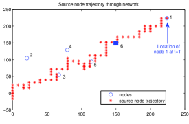
Figure 1: Example 6-node network with mobile source (node 1)

We first find the optimal routing vector by solving (29)-(33) at each time step along the source node trajectory treating the network topology as fixed for that step. Fig. 2 shows the routing vectors during the network lifetime, i.e., the time when the source node depletes its battery (in our numerical examples, we define this to be the time when the source node energy level reaches $10\%$ of its initial energy).

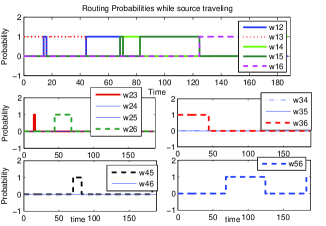
Figure 2: Optimal routing vector for the WSN in Fig. 1 with a mobile source node (Problem II)

The evolution of residual energies of all nodes during the network lifetime is shown in Fig. 3. We can see that at $T=184$ the residual energy of the source node drops to $10\%$ of its initial energy, hence that is the optimal lifetime obtained using the definition where the soft constraint $\sum_{i=1}^{N-1}r_{i}(T)$ is included in (25).

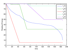
Figure 3: Residual energies over time during the network lifetime

Next, we use the WSN definition where $\sum_{i=1}^{N-1}r_{i}(T)=0$ is used as a hard constraint. As already discussed, the corresponding problems (39) over the source node trajectory are generally infeasible. Instead, we adopt the shortest path routing policy at each step to exploit Theorem 3 with the understanding that the result (for this particular WSN definition) is suboptimal. We consider the same source node trajectory as in Fig. 1. The optimal routing vector updates are shown in Fig. 4, while Fig. 5 shows the residual energy of the nodes during the network lifetime, which in this case is $T=188.49$, slightly longer than the one obtained in Fig. 3 with considerably less computational effort. Also, note that since the source node always sends data packets through the shortest path, it never uses nodes 2 and 4 for this particular trajectory. As expected, (37)-(38) is not feasible, however finding the shortest path at each step in fact improves the network lifetime in the sense of the first time when the source node depletes its energy. We point out, however, that this is not always the case and several additional numerical examples show that this depends on the actual trajectory relative to the relay node locations.

Recall that $\epsilon$ is the weight of the soft constraint in problem $\mathbf{P2(}t\mathbf{)}$. Applying small or large $\epsilon$ makes the problem closer to $\mathbf{P1(}t\mathbf{)}$ or $\mathbf{P3(}t\mathbf{)}$ respectively, e.g. $\epsilon=0.5$ results in $T=190$, however $\epsilon=8$ shrinks the lifetime to $T=156$ suggesting that it is not optimal in this scenario to encourage the nodes to die simultaneously.

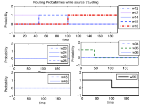
Figure 4: Optimal routing vectors for the WSN in Fig. 1 with a mobile source node (Problem III)

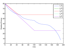
Figure 5: Residual energies over time during the network lifetime

Based on the numerical results, it is obvious that the definition of a static WSN lifetime is not appropriate here. Finally, we observe that the routing vectors are such that at each time step a subset of nodes is fully used ($w_{ij}=1$) while the rest are not used at all. This suggests the possibility of a “bang-bang” type of optimal routing policy, which deserves further investigation.

V Optimal Control Formulation when source node trajectory is known in advance

In this section, we consider the case when we have full advance knowledge of the source node trajectory and include this information in the optimal control problem. Defining the WSN lifetime to be the time when the source node depletes its energy, i.e., using the definition in Problem I, Section IV-A, the problem is formulated as follows:

$$\min_{w(t)}-\int_{0}^{T}dt$$ (40)

$$\text{s.t. }\dot{r}_{i}(t)=-I_{i}(w(t)),\text{ }r_{i}(0)=R_{i},\ \ i=0,..,N-1$$ (41)

$$\begin{bmatrix}\dot{x}_{0}(t)\\ \dot{y}_{0}(t)\\ \end{bmatrix}=\begin{bmatrix}f_{x}(x_{0}(t),y_{0}(t))\\ f_{y}(x_{0}(t),y_{0}(t))\\ \end{bmatrix},\ \ (x_{0}(0),y_{0}(0))\text{ given}$$ (42)

$$I_{i}(w(t))=G_{i}(w(t))[\sum_{j\in O(i)}w_{ij}(t)(C_{s}d_{i,j}^{2}+C_{f})+C_{r}],$$

$$\quad\quad i=1,...,N-1$$ (43)

$$I_{0}(w(t))=\sum_{j\in O(0)}w_{0j}(t)(C_{s}d_{0,j}^{2}(t)+C_{f})$$ (44)

$$G_{i}(w(t))={\displaystyle\sum\limits_{k\in I(i)}}w_{ki}(t)G_{k}(w(t)),\text{ }i=1,..,N-1$$ (45)

$$\sum_{j\in O_{i}}w_{ij}(t)=1,\quad 0\leq w_{ij}(t)\leq 1,i=0,\ldots,N-1$$ (46)

$$r_{0}(T)=0$$ (47)

$$r_{0}(t)>0,\ t\in[0,T);\text{ }r_{i}(t)\geq 0,\text{ }i=1,..,N-1,\text{ }t\in[0,T]$$ (48)

where (42) specifies the trajectory of the source node. In this problem, the state variables are the residual node energies, $r_{i}(t)$, as well as the source node location at time $t$, $(x_{0}(t),y_{0}(t))$. Similar to Section IV-A, we obtain the Hamiltonian:

$$H(w,t,\lambda)=-1+\lambda_{0}(t)(-I_{0}(t))+\sum_{i=1}^{N-1}\lambda_{i}(t)(-I_{i}(t))+$$

$$\lambda_{x}(t)f_{x}(x_{0}(t),y_{0}(t))+\lambda_{y}(t)f_{y}(x_{0}(t),y_{0}(t))$$ (49)

As before, $\lambda_{i}(t)$ is the costate corresponding to $r_{i}(t),\ i=0,...,N-1$ and we add $\lambda_{x}(t)$, $\lambda_{y}(t)$ to be the costates of $x_{0}(t)$ and $y_{0}(t)$. Since we now know the equation of motion for the source node in advance, this imposes terminal constraints for the location of the source node at $t=T$. Thus, based on the dynamics in (42) we can specify $x_{0}(T)$ and $y_{0}(T)$ as $x_{0}(T)=F_{x_{0}}(T)\text{ and }y_{0}(T)=F_{y_{0}}(T)$. Therefore, the terminal state constraint is:

$$\Phi(\mathbf{r}(T),x_{0}(T),y_{0}(T))=$$

$$\nu r_{0}(T)+\mu_{x}(x_{0}(T)-F_{x_{0}}(T))+\mu_{y}(y_{0}(T)-F_{y_{0}}(T))$$ (50)

where $\nu,\ \mu_{x},\ \text{and}\ \mu_{y}$ are unknown constants. It is straightforward to show that $\lambda_{i}(t)$, $i=1,...,N-1$ are as in (15). On the other hand, $\lambda_{x}$ and $\lambda_{y}$ must satisfy:

$$\dot{\lambda}_{x}(t)=-\dfrac{\partial H}{\partial x_{0}}=2C_{s}\lambda_{0}(t)\sum_{j\in O(0)}[w_{0j}(t)(x_{0}(t)-x_{j})]$$

$$-\lambda_{x}(t)\dfrac{\partial f_{x}}{\partial x_{0}}-\lambda_{y}(t)\dfrac{\partial f_{y}}{\partial x_{0}}$$ (51)

$$\dot{\lambda}_{y}(t)=-\dfrac{\partial H}{\partial y_{0}}=2C_{s}\lambda_{0}(t)\sum_{j\in O(0)}[w_{0j}(t)(y_{0}(t)-y_{j})]$$

$$-\lambda_{x}(t)\dfrac{\partial f_{x}}{\partial y_{0}}-\lambda_{y}(t)\dfrac{\partial f_{y}}{\partial y_{0}}$$ (52)

with boundary conditions:

$$\lambda_{x}(T)=\dfrac{\partial\Phi(\mathbf{r}(T),x_{0}(T),y_{0}(T))}{\partial x_{0}(T)}=\mu_{x}$$ (53)

$$\lambda_{y}(T)=\dfrac{\partial\Phi(\mathbf{r}(T),x_{0}(T),y_{0}(T))}{\partial y_{0}(T)}=\mu_{y}$$ (54)

The transversality condition $H(T)+\left.\dfrac{\partial\Phi}{\partial t}\right|_{t=T}=0$ gives:

$$-1+\nu\dot{r}_{0}(T)+\lambda_{x}(T)\dot{x}_{0}(T)+\lambda_{y}(T)\dot{y}_{0}(T)+\nu\dot{r}_{0}(T)+$$

$$\mu_{x}\dot{x}_{0}(T)-\mu_{x}\dfrac{dF_{x_{0}}(T)}{dT}+\mu_{y}\dot{y}_{0}(T)-\mu_{y}\dfrac{dF_{y_{0}}(T)}{dT}=0$$ (55)

The solution of this problem is computationally challenging. Adjoining the control constraints (46) to the Hamiltonian, the problem can be numerically solved using a TPBVP solver, which, fortunately, can be done off line in advance of the source node initiating its known trajectory. It is also possible that the solution is characterized by structural properties (at least for some $f_{x}(x_{0}(t),y_{0}(t))$, $f_{y}(x_{0}(t),y_{0}(t))$) which we plan to investigate in followup work.

VI Conclusions and future work

We have redefined the lifetime for WSNs with a mobile source node to be the time until the source node runs out of energy. When the mobile node’s trajectory is unknown in advance, we have shown that optimal routing vectors can be evaluated as solutions of a sequence of NLPs as the source node trajectory evolves. When the mobile node’s trajectory is known in advance, we have limited ourselves to formulating an optimal control problem which requires an explicit off-line numerical solution. Ongoing work focuses on further exploring this case and on extensions to multiple mobile source nodes.

References

- [1] S. Megerian and M. Potkonjak, Wireless Sensor Networks, ser. Wiley Encyclopedia of Telecommunications. New York, NY: Wiley-Interscience, January 2003.
- [2] V. Shnayder, M. Hempstead, B. Chen, G. W. Allen, and M. Welsh, “Simulating the power consumption of large-scale sensor network applications,” in SenSys ’04: Proceedings of the 2nd international conference on Embedded networked sensor systems. New York, NY, USA: ACM Press, 2004, pp. 188–200.
- [3] C. E. Perkins and P. Bhagwat, “Highly dynamic destination-sequenced distance-vector (dsdv) routing for mobile computers,” in ACM SIGCOMM, 1994, pp. 234–244.
- [4] V. D. Park and M. S. Corson, “A highly adaptive distributed routing algorithm for mobile wireless networks,” in Proc. Of IEEE INFOCOM, 1997, pp. 1405–1413.
- [5] X. Wu and C. G. Cassandras, “A maximum time optimal control approach to routing in sensor networks,” in Proceedings of the 44th IEEE Conference on Decision and Control, and the European Control Conference 2005, Seville, Spain, December 12-15 2005, pp. 1137–1142.
- [6] J.-H. Chang and L. Tassiulas, “Maximum lifetime routing in wireless sensor networks,” IEEE/ACM Transactions on Networking, vol. 12, no. 4, pp. 609–619, August 2004.
- [7] K. Akkaya and M. Younis, “A survey of routing protocols in wireless sensor networks,” Elsevier Ad Hoc Network Journal, vol. 3, no. 3, pp. 325–349, 2005.
- [8] J. Rezazadeh, M. Moradi, and A. S. Ismail, “Mobile wireless sensor networks overview,” Int. j. of Computer Communications and Networks, vol. 2, pp. 17–22, 2012.
- [9] Z. M. Wang, S. Basagni, E. Melachrinoudis, and C. Petrioli, “Exploiting sink mobility for maximizing sensor networks lifetime,” in 38th Hawaii International Conference on System Sciences, 2005.
- [10] R. C. Shah, S. Roy, S. Jain, and W. Brunette, “Data mules: Modeling a three-tier architecture for sparse sensor networks,” in 2 nd ACM International Workshop on Wireless Sensor Networks and Applications, 2003, pp. 30–41.
- [11] M. Di Francesco, S. K. DAS, and G. Anastasi, “Data collection in wireless sensor networks with mobile elements: A survey,” ACM Transactions on Sensor Networks, vol. 8, 2011.
- [12] W. Srinivasan and K.-C. Chua, “Trade-offs between mobility and density for coverage in wireless sensor networks,” in 13th ACM Int. Conf. on Mobile Computing and Networking, 2007, pp. 39–50.
- [13] A. Raja and X. Su, “Mobility handling in mac for wireless ad hoc networks,,” Wirel. Commun. Mob. Comput., vol. 9, p. 303–311, 2009.
- [14] M. Laibowitz and J. Paradiso, “Parasitic mobility for pervasive sensor networks,” in 3rd International Conference on Pervasive Computing, 2005, pp. 255–278.
- [15] K. Dantu, M. Rahimi, H. Shah, S. Babe, and A. D. ansG. Sukhatme, “Robomote: enabling mobility in sensor networks,” in Proc. of 4th Int. Symp. on Information Processing in Sensor Networks, 2005, pp. 404– 409,.
- [16] C. G. Cassandras, T. Wang, and S. Pourazarm, “Optimal routing and energy allocation for lifetime maximization of wireless sensor networks with nonideal batteries,” IEEE Transactions on Control of Network Systems, vol. 1, pp. 86–98, 2014.