Shapley Supercluster Survey: construction of the photometric catalogues and $i$-band data release.

Abstract

The Shapley Supercluster Survey is a multi-wavelength survey covering an area of $\sim$23 deg² ($\sim$ 260 Mpc² at z=0.048) around the supercluster core, including nine Abell and two poor clusters, having redshifts in the range 0.045-0.050. The survey aims to investigate the role of the cluster-scale mass assembly on the evolution of galaxies, mapping the effects of the environment from the cores of the clusters to their outskirts and along the filaments. The optical ($ugri$) imaging acquired with OmegaCAM on the VLT Survey Telescope is essential to achieve the project goals providing accurate multi-band photometry for the galaxy population down to m*+6. We describe the methodology adopted to construct the optical catalogues and to separate extended and point-like sources. The catalogues reach average 5$\sigma$ limiting magnitudes within a 3$\arcsec$ diameter aperture of $ugri$=[24.4,24.6,24.1,23.3] and are 93% complete down to $ugri$=[23.8,23.8,23.5,22.0] mag, corresponding to $\sim$ m*_r+8.5. The data are highly uniform in terms of observing conditions and all acquired with seeing less than 1.1 arcsec full width at half-maximum. The median seeing in $r$-band is 0.6 arcsec, corresponding to 0.56 kpc h${}^{-1}_{70}$ at z=0.048. While the observations in the $u$, $g$ and $r$ bands are still ongoing, the $i$-band observations have been completed, and we present the $i$-band catalogue over the whole survey area. The latter is released and it will be regularly updated, through the use of the Virtual Observatory tools. This includes 734,319 sources down to $i$=22.0 mag and it is the first optical homogeneous catalogue at such a depth, covering the central region of the Shapley supercluster.

1 Introduction

The main aim of the Shapley Supercluster Survey (ShaSS) is to quantify the influence of hierarchical mass assembly on galaxy evolution and to follow such evolution from filaments to cluster cores, identifying the primary location and mechanisms for the transformation of spirals into S0s and dEs. The most massive structures in the local Universe are superclusters, which are still collapsing with galaxy clusters and groups frequently interacting and merging, and where a significant number of galaxies are encountering dense environments for the first time. The Shapley supercluster (hereafter SSC) was chosen because of i) the peculiar cluster, galaxy and baryon overdensities (Scaramella et al., 1989; Raychaudhury, 1989; Fabian, 1991; Raychaudhury et al., 1991; De Filippis, Schindler & Erben, 2005); ii) the relative dynamical immaturity of this supercluster and the possible presence of infalling dark matter haloes as well as evidence of cluster-cluster mergers (e.g. Bardelli et al., 1994; Quintana et al., 1995; Bardelli et al., 1998a, b; Kull & Böhringer, 1999; Quintana, Carrasco & Reisenegger, 2000; Bardelli, Zucca & Baldi, 2001; Drinkwater et al., 2004); iii) the possibility that it is the most massive bound structure known in the Universe, at least in the 10 Mpc central region (see Pearson & Batuski, 2013). These characteristics make the SSC an ideal laboratory for studying the impact of hierarchical cluster assembly on galaxy evolution and to sample different environments (groups, filaments, clusters). Furthermore, the redshift range of this structure (0.033$<z<$0.060 Quintana et al., 1995, 1997; Proust et al., 2006) makes it feasible to measure the properties of member galaxies down to the dwarf regime, providing that the observations reach the suitable depth. A detailed discussion of the scientific aspects of the survey is given in Merluzzi et al. (2015).

Although, the SSC has been investigated by numerous authors since its discovery (Shapley 1930) both for its cosmological implications (Scaramella et al., 1989; Raychaudhury, 1989; Plionis & Valdarnini, 1991; Quintana et al., 1995; Kocevski, Mullis & Ebeling, 2004; Feindt et al., 2013, and references therein) and for studies of cluster-cluster interactions (e.g. Kull & Böhringer, 1999; Bardelli et al., 2000; Finoguenov et al., 2004; Rossetti et al., 2005; Muñoz & Loeb, 2008), none of them could systematically tackle the issue of galaxy evolution in the supercluster environment due to the lack of accurate and homogeneous multi-band imaging covering such an extended structure. ShaSS aims to fill this gap measuring the integrated [magnitudes, colours, star formation rates (SFRs)] and internal (morphological features, internal colour gradients) properties of the supercluster galaxies.

ShaSS will map a region of $\sim$ 260 h${}_{70}^{-2}$ Mpc² (at z=0.048), centred on the SSC core, which is constituted by three Abell clusters: A 3558 (z=0.048, Melnick & Quintana 1981, Metcalfe, Godwin & Spenser 1987; Abell richness $R$=4, Abell, Corwin & Olowin 1989), A 3562 (z=0.049, $R$=2) and A 3556 (z=0.0479, $R$=0); and two poor clusters SC 1327-312 and SC 1329-313. The present survey covers also six other Abell clusters: A 3552, A 3554, A 3559, A 3560, AS 0724, AS 0726, as shown in Fig. 1. The survey boundaries are chosen not only to cover all 11 clusters and the likely connecting filaments, but also to extend into the field and to map the structures directly connected to the SSC core. In Merluzzi et al. (2015) we derived the stellar mass density distribution based on supercluster members showing that all the clusters in the ShaSS area are embedded in a common network and identified a filament connecting the SSC core and the cluster A 3559 as well as the less pronounced overdensity extending from the SSC core towards A 3560.

The data set of the survey includes optical ($ugri$) and NIR ($K$) imaging acquired with (VST) and Visible and Infrared Survey Telescope for Astronomy (VISTA) respectively, and optical spectroscopy with AAOmega. At present the $i$-band imaging and AAOmega spectroscopic surveys are completed, while the other observations are ongoing. In addition, the recent public release of data from the Wide-field Infrared Survey Explorer ($WISE$, Wright et al., 2010) provides photometry at both near-IR (3.4,4.6 $\mu$m) and mid-IR (12,22 $\mu$m) wavelengths, allowing independent measurements of stellar masses down to $\mathcal{M}$=10⁹M_⊙ at 10$\sigma$ and SFR down to 0.46 M_⊙yr^-1 at 10$\sigma$ (0.2 M_⊙yr^-1 at 5$\sigma$). Finally, in the 2–3 deg² of the SSC core, panoramic imaging in the UV (Galaxy Evolution Explorer, GALEX), optical (ESO Wide Field Imager, WFI), NIR (UKIRT/WFCAM) and mid-infrared (Spitzer/MIPS) are also available (Mercurio et al., 2006; Merluzzi et al., 2010; Haines et al., 2011).

The optical survey, whose coverage is indicated by the 1 deg² boxes in Fig. 1, will enable us to i) derive accurate morphologies, structural parameters ($\delta$log$r_{e}\sim 0.04$ and $\delta n_{Ser}\sim 1$) as well as detect some of the observational signatures related to the different processes experienced by supercluster galaxies (e.g. extraplanar material); ii) estimate accurate colours, photo-zs ($\delta z<0.03$, see Christodoulou et al., 2012) and stellar masses; iii) evaluate the SFRs and resolve the star forming regions at least for the subsample of brighter galaxies.

The survey depth enables global and internal physical properties of Shapley galaxies to be derived down to $m^{\star}$+6. In the first case of obtaining accurate measurements of aperture photometry and colours, we require signal-to-noise ratios (SNR) of 20 in all four bands for SSC galaxies down to $m^{\star}$+6. Secondly, for the morphological analysis and resolving internal properties and structures there is a more stringent requirement of SNR$\sim$100 (in a 3$\arcsec$ diameter aperture, see Conselice, Bershady & Jangren, 2000; Häussler et al., 2007) for the deeper $r$-band imaging. For this reason we are collecting the $r$-band imaging under the best observing conditions, with a full width at half-maximum (FWHM)$\sim$0.8 arcsec or better, corresponding to 0.75 kpc at z=0.048. Additionally, the $r$ imaging is fundamental to our weak lensing analysis, to ensure a sufficient density of lensed background galaxies with shape measurements.

With these data it will be possible to separate the different morphological types, trace ongoing SF, reveal recent interaction or merging activities and thus obtain a census of galaxies whose structure appears disturbed by the environment (e.g. Scarlata et al., 2007; Muñoz-Mateos et al., 2009; Kleiner et al., 2014; Holwerda et al., 2014; Lotz et al, 2008, 2011, and references therein).

In order to achieve the scientific goals of the survey, accurate photometry is required. This implies a clean source catalogue containing, together with the measured photometric properties, indicators of the reliability of these measurements. This paper describes the methodology used to produce the photometric catalogues and the adopted procedures.

Observations are overviewed in Sect. 2. In Sect. 3 we describe the construction of the catalogues, the criteria to classify spurious objects and unreliable detections, the flags adopted in the catalogues and the procedure for star/galaxy separation. The accuracy and completeness of the derived photometry is discussed in Sect. 4. Each parameter of the released $i$-band catalogues is detailed in Sect. 5 and the summary is given in Sect. 6.

Throughout the paper, we assume a cosmology with $\Omega_{\mathrm{m}}$= 0.3, $\Omega_{\mathrm{\Lambda}}$= 0.7 and H₀= 70 km s^-1 Mpc⁻¹. According to this cosmological model 1  arcmin corresponds to 56.46 kpc at z=0.048. The magnitudes are given in the AB photometric system.

2 VST observations and data reduction

The optical survey (PI: P. Merluzzi) is being carried out using the Italian INAF Guaranteed Time of Observations (GTO) with OmegaCAM on the 2.6m ESO VLT Survey Telescope located at Cerro Paranal (Chile). The Camera has a corrected field of view of 1${}^{\circ}\times$1^∘, corresponding to $\sim$ 3.4$\times$3.4 h${}_{70}^{-2}$ Mpc² at the supercluster redshift, sampled at 0.21 arcsec per pixel with a 16k$\times$16k detector mosaic of 32 CCDs, with gaps of 25-85 arcsec in between chips .

Each field is observed in four bands: $ugri$. To achieve the required depth, total exposure times for each pointing are 2955s in $u$, 1400s in $g$, 2664s in $r$ and 1000s in $i$. To bridge the gaps a diagonal dither pattern of five exposures in $u$, $g$ and $i$, and nine exposures in $r$ is performed, with step size of 25$\arcsec$ (15 $\arcsec$ for the $r$ band) in X, and 85$\arcsec$ (45$\arcsec$ in $r$) in the Y-direction. The total area is covered by 23 contiguous VST pointings overlapping by $\sim$3$\arcmin$ as shown in Fig. 1, where dots denote the spectroscopic supercluster members ($13500<V_{h}<16000$ km s^-1) available from literature at the time of the survey planning. The X-ray centres are indicated by crosses for all the known clusters except AS 0726, whose centre is derived by a dynamical analysis.

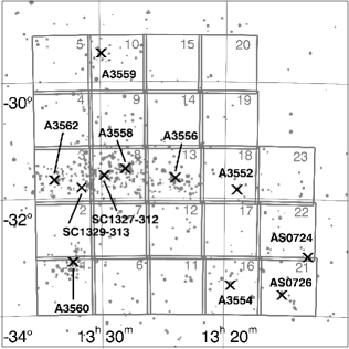
Figure 1: VST fields mapping the ShaSS region. Dots indicate the supercluster members in the range v_heliocentric=13500-16000 km s⁻¹, taken from literature. Note that the literature redshift coverage is not uniform across the region shown. Black crosses show the cluster centres.

The survey started in 2012 February and will be completed in 2015 (spanning ESO periods P88-P95), provided that all the foreseen observations are carried out. At present, the survey coverage differs for each band with only the $i$-band observations available for the whole area. This implies that the results concerning the quality of the photometry (depth, completeness, accuracy) are based on a representative subsample of the final catalogues for $ugr$ (48%, 43% and 61%, respectively) bands and for the whole catalogue in $i$ band.

The data are collected on clear and photometric nights with good and uniform seeing conditions. In Fig. 2 we plot the seeing values of 11, 10, 14 and 23 fields in $ugri$, respectively. Out of the observed fields about 80% ($gi$) and 90% ($r$) are acquired with FWHM$\leq$ 0.8 arcsec, with the median seeing in $r$ band equal to 0.6 arcsec, corresponding to 0.56 kpc h${}^{-1}_{70}$ at z=0.048. The $u$ band is characterized by a slightly poorer seeing. We discuss the effect of the seeing on the aperture magnitudes in Sect. 3.1.2.

Figure 2: Seeing distribution in the four observed bands (see text).

The data reduction is already described in Merluzzi et al. 2015. Here we summarize the main steps for the reader’s convenience.

Images are reduced and combined using the VST–Tube imaging pipeline (Grado et al. 2012), developed ad hoc for the VST data. The pipeline follows the standard procedures for bias subtraction and flat-field correction. A normalized combination of the dome and twilight flats, in which the twilight flat is passed through a low-pass filter first, were used to create the master flat. A gain harmonization procedure has been applied, finding the relative CCD gain coefficients which minimizes the background level differences in adjacent CCDs. A further correction is applied to account for the light scattered by the telescope and instrumental baffling. This is an additional component to the background, which, if not corrected for, causes a position-dependent bias in the photometric measurements. This component is subtracted through the determination and the application of the illumination correction (IC) map. The IC map is determined by comparing the magnitudes of photometric standard fields with the corresponding SDSS-DR8 (Sloan Digital Sky Survey-Data Release 8) PSF magnitudes.

For the $i$ band a correction is required because of the fringe pattern due to thin-film interference effects in the detector from sky emission lines. The fringing pattern is estimated as the ratio between the Super-Flat and the twilight sky flat, where Super-Flat is obtained by overscan and bias correcting a sigma clipped combination of science images. The fringe pattern is subtracted from the image, applying a scale factor which minimizes the absolute difference between the peak and valley values (maximum and minimum in the image background) in the fringe corrected image.

The photometric calibration onto the SDSS photometric system is performed in two steps: first a relative photometric calibration among the exposures contributing to the final mosaic image is obtained through the comparison of the magnitudes of the bright unsaturated stars in the different exposures, using the software SCAMP (Bertin 2006); then the absolute photometric calibration is computed on the photometric nights comparing the observed magnitude of stars in photometric standard fields with SDSS photometry. For those fields observed on clear nights, we take advantage of the sample of bright unsaturated stars in the overlapping region between clear and photometric pointings and by using SCAMP, each exposure of the clear fields is calibrated on to the contiguous photometrically calibrated field. The magnitude is then calibrated by adopting the following relation:

$$M^{\prime}=M+\gamma C+AX+ZP,$$ (1)

where $M$ is the magnitude of the star in the standard system, $M^{\prime}$ is the instrumental magnitude, $\gamma$ is the coefficient of the colour term, $C$ is the colour of the star in the standard system, $A$ is the extinction coefficient, $X$ is the airmass and $ZP$ is the zero-point. The results are reported in Table 1.

Band	Colour term	Colour	Extinction	Zero Point
			Coefficient
$M$	$\gamma$	$C$	$A$	$ZP$
$u$	0.026$\pm$0.019	u-g	0.538	23.261$\pm$0.028
$g$	0.024$\pm$0.006	g-i	0.180	24.843$\pm$0.006
$r$	0.045$\pm$0.019	r-i	0.100	24.608$\pm$0.007
$i$	0.003$\pm$0.008	g-i	0.043	24.089$\pm$0.010

Table 1: Absolute photometric calibration coefficients.

To further check our photometric calibration, in particular for stars in fields observed in clear nights, we derive the median stellar loci of SDSS and ShaSS stars in ($g-r$, $r-i$) colour-colour space (see Fig. 3). The distance between the two loci, over the whole range of colours, never exceeds 0.015 mag, which is less than the expected error on colours.

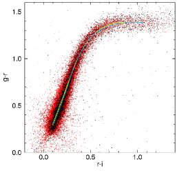
Figure 3: Colour-colour ($g$-$r$,$r$-$i$) diagram showing a sample of stars from ShaSS (black dots) overimposed on a sample of SDSS stars (red dots). The curves trace the loci of the stars in the plane (ShaSS: cyan; SDSS: yellow). The distance between the curves never exceeds $\sim$0.015 mag.

When photometric calibration is performed, the background is removed with the software SWARP (Bertin et al. 2002), which also standardizes the zero-point to a value of 30.0 mag.

3 Catalogue construction and star/galaxy classification

The procedure adopted for the source extraction is optimized for the goals of the survey. Due to the image depth, sources span a wide range of size, luminosity and morphology, and thus we need a multifaceted approach to obtain robust measures of their aperture and total magnitudes. Moreover, the SSC is located at relatively low galactic latitude ($b\sim$30), which implies the presence of a large number of stars across the survey area, making the star/galaxy classification a crucial issue for the catalogue’s construction.

The photometric catalogues are produced using the software SExtractor (Bertin & Arnouts, 1996) in conjunction with PSFEx (Bertin, 2011), which performs PSF fitting photometry. We extract independent catalogues in each band, which are then matched across the four wavebands using STILTS (Taylor 2006).

3.1 Catalogue construction

The procedure adopted for source extraction aims: i) to detect as many sources as possible, while minimizing the contribution from spurious objects, ii) to produce accurate measurements of positions and photometric quantities, iii) to flag objects in the haloes of bright stars and hence could have had their photometry affected. During the construction of the catalogues, the results have been always visually inspected on the images to check the residual presence of spurious objects or misclassified objects, like traces of satellites, fake objects due to cross-talk, effects of bad columns.

3.1.1 Source detection

Sources included in the final catalogue are extracted in four steps: i) sky background modelling and subtracting, ii) image filtering, iii) thresholding and image segmentation, iv) merging and/or splitting of detections.

In order to optimize the automatic background estimation, we obtained catalogues by adopting different BACK_SIZE and BACK FILTERSIZE and compared sources extracted in each catalogue, both in terms of number of spurious detections and photometric quantities, such as aperture and Kron magnitudes and flux radius. Finally, given the average size of the objects, in pixels, in our images, and in order to minimize the number of spurious detections, we set the BACK_SIZE and BACK FILTERSIZE to 256 and 4 respectively, for all fields and bands. To get accurate background values for the photometry, the background is also recomputed in an area centred around the object in question, setting BACKPHOTO_TYPE to LOCAL and the thickness of the background LOCAL annulus (BACKPHOTO_THICK) to 24.

Once the sky background is subtracted, the image must be filtered to detect sources. To determine whether the Gaussian or top-hat filter was optimal for our scientific objectives, a specific analysis was carried out on the $g$-, $r$- and $i$-band images for field 8. The catalogues produced using the top-hat filter were found to contain more spurious sources than those with the Gaussian filter, while the photometric measurements as well as the completeness of the catalogues were confirmed to be equivalent. Finally we chose to apply the Gaussian filter (gauss_3.0_5x5.conv).

The detection process is mostly controlled by the thresholding parameters (DETECT_THRESHOLD and ANALYSIS_THRESHOLD). The choice of the threshold must be carefully considered. A too high threshold results in the loss of a high number of sources in the extracted catalogue, while a too low value leads to the detection of spurious objects. Hence, a compromise is needed by setting these parameters according to the image characteristics, the background rms, and also to the final scientific goal of the analysis.

For our analysis, the threshold value was chosen to maximize the number of detected sources, while simultaneously keeping the number of spurious detections to a minimum. To identify the optimal threshold value, we counted the number of extracted sources for different threshold values in 1 deg² $r$-band image and the corresponding negative image, which is the scientific image multiplied by -1. As the threshold decreases, the number of detected sources (real plus spuriuos detections) increases, as shown in the left-hand panel of Fig. 4. In the negative image (right panel of Fig. 4) the number of sources (spurious detections in this case) increases smoothly down to a certain value of the threshold, beyond which it shows a dramatic change in steepness. The suitable threshold value corresponds to this change in the trend of source number counts. As pointed out above, the catalogue was visually inspected to avoid residual spurious detections and to verify the deblending parameters.

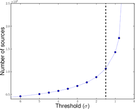
(a)

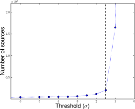
(b)

Figure 4: Number of extracted sources for the $r$-band image (left-hand panel) and negative image (right-hand panel, see text) of field 12 as a function of the SExtractor threshold. The dashed vertical line indicates in both panels the adopted detection threshold.

Two or more very nearby sources can be mistakenly detected as a unique connected region of pixels above threshold and, in order to correct for this effect, SExtractor adopts a deblending method based on a multi-thresholding process. Each extracted set of connected pixels is re-thresholded at $N$ levels, linearly or exponentially spaced between the initial extraction threshold and the peak value. Also here we should find a compromise for the deblending parameter, since too high a value leads to a lack of separation between close sources, while too low a value leads to split extended spiral galaxies into several/multiple components.

In general, the choice of the deblending (but also the threshold) parameter is related to the main scientific interest. If we are mostly interested in the analysis of faint and small objects, we have to fix low values for deblending and threshold parameters, at the cost of splitting up the occasional big bright spiral galaxy into many pieces. On the other hand, by fixing larger values for deblending and threshold parameters, we correctly deblend the larger objects, but we lose depth. However, the present data cover large areas and the science involves the analysis of both large and bright as well as faint and small galaxies.

Parameter	Values
DETECT_MINAREA	5
DETECT_THRESH	1.5$\sigma$
ANALYSIS_THRESH	1.5$\sigma$
DEBLEND_NTHRESH	32
DEBLEND_MINCONThot	0.001
DEBLEND_MINCONTcold	0.01
BACK_SIZE	256
BACK_FILTERSIZE	4

Table 2: Main input parameters set in the SExtractor configuration files. DETECT_MINAREA and BACK_SIZE are expressed in pixels.

For this reason it is not possible to fix a unique value for threshold and deblending parameters, and we used a two-step approach in the catalogue extraction (e.g.: Rix et al. 2004, Caldwell et al. 2008). First, we ran SExtractor in a so called cold mode where the brightest and extended sources are properly deblended; then, in a second step, we set configuration parameters in order to detect fainter objects and to properly split close sources (hot mode). We combined the two catalogues by replacing extended objects, properly deblended in cold mode, in the catalogue of sources detected in the hot mode, and by deleting multiple detections of these extended sources. In order to combine these two catalogues we compare the segmentation maps obtained with $cold$ and $hot$ modes. First we flagged the different objects detected in the hot mode, but lying inside the Kron area of the same object detected in cold mode, which are typically 80–120 per field. These objects are, in general, large spiral galaxies, galaxies with superimposed smaller galaxies or stars and close objects not properly deblended in cold mode. From the visual inspection of all the flagged objects we chose cold mode detection for spiral galaxies and hot mode for other cases. The main values set for SExtractor are listed in Table 2.

3.1.2 Aperture photometry and total magnitudes

Measurements of position, geometry, and photometric quantities are included in the final catalogues for all the detected and properly deblended sources. Among the photometric quantities calculated are: aperture magnitudes (MAG_APER), measured in 10 circular apertures whose fixed diameters are reported in Table 3; isophotal magnitudes (MAG_ISO), computed by considering the threshold value as the lowest isophote and using two different elliptical apertures: the Kron (MAG_AUTO, Kron 1980) and the Petrosian (MAG_PETRO, Petrosian 1976) magnitudes, which are both estimated through an adaptive elliptical aperture. The adopted Kron and Petrosian factors, and the minimum radius fixed for the elliptical apertures are reported in Table 3 (PHOT_AUTOPARAMS and PHOT_PETROPARAMS, respectively).

In order to test the effect of seeing on the aperture magnitudes we used the program SYNMAG (Bundy et al., 2012). With this software we can input magnitudes, effective radii and Sérsic indices to obtain the synthetic magnitude of the source inside an aperture of fixed radius. We found that for photometry measured within fixed apertures of 8 $\arcsec$ diameter, the level of flux lost remains below 0.02 mag for both exponential (n_Sersic=1) and de Vaucouleurs (n_Sersic=4) profiles, for seeing levels in the range 0.5-1.1 arcsec and effective radii in the range 3.0-100.0 arcsec.

Parameter	Values
PHOT_APERTURES	1.5,3.0,4.0,8.0,16.0,30.0,45.0,90.0
PHOT_APERTURES	3*FWHM,8*FWHM
PHOT_AUTOPARAMS	2.5, 3.5
PHOT_PETROPARAMS	2.0, 3.5

Table 3: Adopted aperture diameters, MAG_AUTO and MAG_PETRO parameters. PHOT_APERTURES are expressed in arcsec (first row) and as a function of the measured FWHM (second row).

To describe the size of the sources we extract: the half flux radius, i.e. the FLUX_RADIUS containing the 50% of the total light and that containing the 90% of the light. We also measured the PETRO_RADIUS, defined as the point in the radial light profile at which the isophote at that radius is 20% of the average surface brightness within that radius, and the KRON_RADIUS, which is the characteristic dimension of the ellipse used to calculate the KRON_MAGNITUDE. The Kron and the Petrosian magnitudes are measured within elliptical apertures, whose semi-major and semi-minor axes are equal to A_IMAGE and B_IMAGE multiplied by the KRON_RADIUS and PETRO_RADIUS parameters, respectively.

As position parameters, we measured the barycenter coordinates both in pixels (X_IMAGE, Y_IMAGE) and in degrees (ALPHA_J2000, DELTA_J2000), computed as the first order moments of the intensity profile of the image, and the position of the brightest pixel (ALPHAPEAK_J2000, DELTAPEAK_J2000).

3.1.3 Model-derived magnitudes

By using the PSFEx tool Bertin (2011) it is possible to model the PSF of the images. We considered only non-saturated point sources with a SNR higher than 80. Spatial variations of the PSF were modelled with a third degree polynomial of the pixel coordinates. The main values set for PSFEx parameters are given in Table 4. More details on the PSF modelling with the PSFEx tool can be found Bertin (2011), Mohr et al. (2012) and Bouy et al. (2013).

Parameter	Values
BASIS_TYPE	PIXEL_AUTO
BASIS_NUMBER	20
PSF_ACCURACY	0.01
PSF_SIZE	25,25

Table 4: Main input parameters set in the PSFEx configuration file. PSF_SIZE are expressed in pixels.

Hence, it is possible to run SExtractor taking the PSF models as input, using them to carry out the PSF-corrected model fitting photometry for all sources in the image. With a combination of SExtractor and PSFEx, we obtained magnitudes from: (i) the PSF fitting (MAG_PSF and the point source total magnitude MAG_POINTSOURCE); (ii) the fit of a spheroidal component (MAG_SPHEROID); (iii) the fit of a disc component (MAG_DISK); and (iv) the sum of the bulge and the disc components, centred on the same position, convolved with the local PSF model (MAG_MODEL). We also extracted morphological parameters of the galaxies, such as spheroid effective radius (SPHEROID_REFF_IMAGE), spheroid Sérsic index (SPHEROID_SERSICN), spheroid aspect (SPHEROID_ASPECT_IMAGE), disc scale length (DISK_SCALE_IMAGE) and disc aspect (DISK_ASPECT_IMAGE).

The model of the PSF is also helpful to get a more accurate star/galaxy classification (see Sect. 3.3).

3.2 Haloes and spikes of bright stars, and image borders

Multiple reflections in the internal optics of OmegaCAM can produce complex image rings and ghosts (hereafter star haloes) near bright stars . These haloes are characterized by a central region in which the surface brightness is depressed and an outer corona with enhanced surface brightness, both characterized by an irregular pattern as shown in Fig. 5 (left panel) for the $i$-band images. Those haloes all have the same radius of 830 pixels in all bands and the position of their centres is related to the position of the parent star in the OmegaCAM field. The ‘intensity’ (depth of the inner depression and brightness of the corona) of the halo depends on the band, being more manifest in the $i$ band and practically negligible in $u$ band. Moreover, the intensity of the halo is related to the magnitude of the parent star. To quantify this behaviour we assigned a value proportional to the halo masks: mask=INT(100$\times$ i_mag). Notice that parent stars are saturated in our images, so we draw their magnitudes from the USNO-B1.0 catalogue. Whenever two or more haloes overlap, the mask assumes locally the value corresponding to the halo of the brightest star. We limited the creation of masks to stars brighter than $i$=9.6 mag, although the haloes produced by stars with $i>$ 9.0 mag already do not show surface brightness excesses higher than $\sim$0.2 times the r.m.s. of the background. In all 23 VST fields in $i$ band, we identified and masked 299 haloes. In the right panel of Fig. 5 we show an example of a halo mask.

Figure 5: A crowding of five saturated stars with related haloes (left) and the corresponding halo mask (right). The $i$-band magnitudes of the stars are, left to right, 8.77, 8.24, 8.99, 8.56, 7.81. A logarithmic stretch was applied to the image to increase the background. The image corresponds to an area of 9$\arcmin$ $\times$ 6$\arcmin$.

The saturated stars with haloes also affect the images by producing spike features which are masked as follows. First we identified the position of all saturated pixels according to the value corresponding to the SATURATE keyword in the header of each image. Then we applied a region growth algorithm around each saturated pixel to obtain a mask consisting of three levels, corresponding to three threshold values of the surface brightness of 20, 20.5 and 21 mag arcsec^-2. An example of a spike mask is shown in Fig. 6.

The halo and spike masks have been used to flag each source s_i considering the circular area embedding 50% of the flux, A50_i. From both halo and spike masks we derive a couple of flags: i) the fraction of A50_i affected by the halo and/or spike mask; ii) the halo and/or mask value within the affected portion of A50_i.

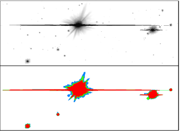
Figure 6: An area containing a star with prominent spikes and other saturated stars (top) and the corresponding spike mask (bottom). The three levels of the mask correspond to three different surface brightness thresholds ($\mu_{i}<$ 21, 20.5, 20 mag arcsec^-2, coded here in blue, green and red respectively). The shown field measures 2.8$\arcmin$ $\times$ 7.7$\arcmin$.

The dither acquisition mode adopted for the observations produces a non-uniform coverage of the co-added image, so that the catalogue of detections covering the whole mosaic image will contain detections from regions with different depths. For a five(nine)-dither pattern at least three(five) exposures cover almost the whole image in $ugi$($r$). Along the borders, however, there are stripes where only 1-2(1-4) exposures contribute to the final co-added mosaic in $ugi$($r$). We decided to exclude these detections from the final catalogues. This cut was possible thanks to the 3^′ overlaps among the contiguous 1 deg² VST fields, which ensure that a common area (and common detections) is present even after the borders are cut. To mask out we empirically identified the external areas with different exposures by just associating a range of values of the weight mask to a number of exposures. An example of an exposure mask is given in Fig. 7. Objects lying in areas with mask values lower than 3(5) are not included in the survey catalogues, except for a very few number of sources located in the gaps among the detectors.

We also excluded those objects for which more than 80% of their pixels (within a circular region with radius equal to 50% flux radius) have zero weight.

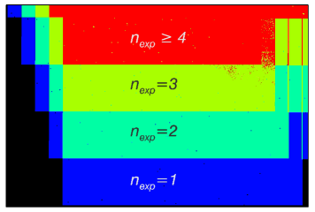
Figure 7: Cutoff of an exposure mask near to a corner of a VST image. The area shown is about 14$\arcmin$ $\times$ 12$\arcmin$. The colours correspond to the different numbers of exposure as indicated.

3.3 Star/Galaxy separation

To separate extended and point-like sources, we adopt a progressive approach analogous to those described in Annunziatella et al. (2013), using the following parameters provided by SExtractor: (i) the stellarity index (CLASS_STAR); (ii) the half-light radius (FLUX_RADIUS); (iii) the new SExtractor classifier SPREAD_MODEL; (iv) the peak of the surface brightness above background ($\mathrm{\mu_{max}}$); (v) a final visual inspection for objects classified as galaxies but with borderline values of the stellarity index (CLASS_STAR$\geq$0.9; see below).

The stellarity index results from a supervised neural network that is trained to perform a star/galaxy classification. It assumes values between 0 and 1. In theory, SExtractor considers objects with CLASS_STAR equal to zero to be galaxies, and those with value equal to one as stars. As an example in Fig. 8a, CLASS_STAR is plotted as a function of the Kron magnitude for $r$-band sources in field 12. The sequence of unsaturated stars ($r>15.5$ mag) is clearly separated from galaxies by selecting a CLASS_STAR value above 0.98 only down to $r$=20.5 mag. For magnitudes fainter than this value, lowering the established limit to separate stars and galaxies causes an increase of the contamination of the star subsample from galaxies. So, we can only adopt this parameter to classify bright sources ($r<$20.5 mag) as stars, when CLASS_STAR$\geq$0.98.

By using (FLUX_RADIUS) as a measure of source concentration, we can extend the classification to fainter magnitudes. Figure 8b shows that the locus of stars, defined according to the relation between half-light radius and Kron magnitude is recognizable down to $r$=22.8 mag. This limit is 0.7 mag brighter than the completeness limit of the $r$-band catalogue (see Sect. 4.3). For this reason we used the new SExtractor classifier, SPREAD_MODEL, which takes into account the difference between the model of the source and the model of the local PSF (Desai et al., 2012), to obtain a reliable star/galaxy classification for the faintest objects in our catalogue. By construction, SPREAD_MODEL is close to zero for point sources, positive for extended sources (galaxies), and negative for detections smaller than the PSF, such as cosmic rays. Figure 8c shows the distribution of the SPREAD_MODEL as a function of Kron magnitude. Stars and galaxies tend to arrange themselves in two different places of the plot distinguishable up to $r$=23.8 that is a limit 0.3 mag fainter than the completeness limit of the catalogue. Based on this diagram, we classified as galaxies all sources with SPREAD_MODEL $>$ 0.005 and $r\leq$23.8, or SPREAD_MODEL $>$ 0.003 and $r>$23.8.

Finally, in Fig. 8d we plot $\mathrm{\mu_{max}}$ as a function of the Kron magnitude. This plot is used in order to select saturated stars (vertical dashed line in all panels of Fig. 8).

Since the $r$ band is the deepest band of the survey, and the one conducted in the best seeing conditions, it will be used for classification of sources in the cross-correlated catalogue of the four bands. The same criteria have also been used for the $i$ and $g$ band independently and the results are consistent.

The star/galaxy separation of the $u$ band relies on the $r$ band, since the nature of the $u$-band emission, which is very sensitive to the presence of SF regions. For this band a careful cross-correlation with the other catalogues is also required since the deblending parameter cannot be suitably calibrated. We will further detail the construction of the $u$-band catalogue in a dedicated article.

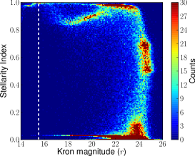
(a)

(b)

(c)

(d)

Figure 8: Two-dimensional histogram of SExtractor stellarity index (panel a), half-light radius (panel b), spread model (panel c), and $\mathrm{\mu_{max}}$ (panel d) as a function of Kron magnitude for sources in $r$-band image of field 12. The vertical dashed line in all panels is the magnitude limit adopted for saturated objects. The horizontal lines in panel c) mark the limit used to separate stars and galaxies (see text). The points are colour coded according to their number counts as reported in the vertical colour bars.

After completing the star/galaxy separation, a visual inspection of those objects classified as galaxies but with CLASS_STAR$\geq$0.9 (which are about 10 per field), is performed.

To check the reliability of the star/galaxy classification in the $i$-band images, we performed simulations by adding artificial stars and galaxies, through a stepwise procedure. To preserve the overall source density, we split the artificial stars and galaxies into eight magnitude bins of width 0.5 mag, over the magnitude range 18$<i<$22, producing eight different simulated images for each real image. To define the PSF we take advantage of the PSF modelled according to PSFEx. To simulate galaxies with dimensions representative of real deep images, we defined the size in pixels of the model in the output image, according to the distribution of the measured half-flux radius as a function of the total magnitude obtained for the real galaxies. We attempted to recover artificial sources by running SExtractor again with the same parameters for object detection and classification as on the original images. We were able to correctly separate 100% of simulated stars and galaxies down to $i$=20.0 mag. We erroneously classify as galaxies 0.8%, 1.5%, 2.1% and 3.0% of stars in the magnitude bins 20.0–20.5, 20.5–21.0, 21.0–21.5 and 21.5–22.0, respectively. All galaxies were correctly recovered down to $i$=21.0, while in the last two magnitude bins just 0.7% and 2.2% were misclassified as stars.

To test if the method adopted to classify stars and galaxies could introduce a bias in the distribution of galaxy sizes we compared our observed distribution of real galaxy sizes, with those derived by using completely independent methods. In particular, we verified that our size distribution for galaxies down to M^∗+6 was in agreement with those of D’Onofrio et al. (2014) for WINGS clusters.

However, compact galaxies might be confused with stars due to their small radii and comparably high surface brightness. Previous studies on the sizes of dwarf and compact dwarf galaxies in Coma (e.g. Graham & Guzman 2003, Price et al. 2009, Hoyos et al. 2011) and in other nearby clusters like Centaurus (Misgeld et al. 2009), Antlia (Smith Castelli et al. 2012), Virgo, Fornax and Perseus (Weinmann et al. 2011) have shown that the effective radii of these galaxies can vary from few kiloparsec to hundreds of parsec. To investigate to what extent we are able to properly distinguish compact galaxies from stars we run ad hoc simulations. We added to the images artificial compact galaxies and used the same detection method as for the real catalogues. Simulated galaxies with a minimum effective radius of 0.7 kpc (i.e. $\sim$ 1 arcsec at z=0.048) are all recovered. Then, considering galaxies with a minimum effective radius of 0.6 kpc, we erroneously classify as stars only 2.2% of compact galaxies. Finally, by simulating galaxies with effective radii down to 0.4 kpc we were able to classify as extended objects 60-70% of galaxies. However, we would like to underline that 400 pc corresponds to $\sim$ 0.4 arcsec at the mean distance of the SSC (z=0.048), so, to assess the nature (star or galaxy) of these objects, we need either a measure of the redshift or to perform a fit to the surface brightness distribution.

4 Photometry

In this section, we will focus on the photometric depth, the accuracy of the derived photometry and the completeness magnitude. All the quantities shown in this section are obtained by excluding saturated stars, sources affected by saturation spikes, stars in haloes of bright stars, and those with less than half the total exposure of the frames, which means that we included the sources with at least three exposures in the ugi bands and with at least five exposures in the r band. We remind the reader that the results for the $u$ band are preliminary.

The results of Sections 4.1 and 4.3 are based on the $ugri$ catalogues including 11, 10, 14 and 23 fields, respectively. For each band we cross-correlate the field catalogues with STILTS selecting in the overlap regions the detection from the image with the best seeing. This criterion is also adopted for producing the final $i$-band catalogue covering the whole ShaSS area.

We also report in Table 5 a summary of the exposure time, median seeing, completeness limits and detection limits at 5$\sigma$ for each band.

Table 5: ShaSS photometry.

Band	Exp. Time	completeness	detection [5$\sigma$]	seeing a)
	[s]	[mag]	[mag]	[arcsec]
$u$	2955	23.8	24.4	0.9
$g$	1400	23.8	24.6	0.7
$r$	2664	23.5	24.1	0.6
$i$	1000	22.0	23.3	0.7

a) Median FWHM estimated from the already observed fields.

4.1 Photometric depth

We estimated the photometric depth of each field by randomly placing 10000 3-$\arcsec$ apertures on the VST image of each field. From the resulting standard deviation in the flux measurements obtained within these apertures, the corresponding 20$\sigma$ and 5$\sigma$ magnitude limits were determined for each image. The mean values obtained in each field are 22.9, 23.1, 22.6, 21.7 in $ugri$ band at 20$\sigma$ and 24.4, 24.6, 24.1, 23.3 in $ugri$ band at 5$\sigma$. The variation of these detection limits across the fields is less than 0.05 in $ug$, and 0.1, 0.2 in $r$ and $i$ band, respectively. Merluzzi et al. (2015) reported slightly different values since they measured the SNR within 3 $\arcsec$ diameter apertures as a function of the magnitude, according to equation (61) of SExtractor User’s Manual, while in this paper we measured the detection limits directly on the images.

4.2 Photometric accuracy

To test the accuracy of our photometry we used the stars in the 3 arcmin wide stripes of overlap between adjacent VST fields. The magnitudes adopted for this comparison are those derived in an 8$\arcsec$ diameter aperture, which ensures that our estimates are not affected by the seeing differences between fields. The average number of stars in each strip are $\sim$650 in $u$ and 1500 in $gri$ bands.

We computed the magnitude difference $\Delta^{ij}_{k}=$m${}^{j}_{k}$- m${}^{i}_{k}$ as a function of mag${}^{ij}_{k}=\frac{1}{2}\times$(m${}^{i}_{k}$+m${}^{j}_{k}$) for all stars belonging to each pair $ij$ of adjacent frames. Here $i$ and $j$ identify the different VST fields and $k$ refers to the stars, so that m${}^{j}_{k}$ is the magnitude of the $k$-th star in field $i$ and $\Delta^{ij}_{k}$ is the difference in magnitude of the $k$-th star between fields $j$ and $i$.

To estimate the uncertainties on magnitudes, we collected the absolute values of the differences $\left|\Delta^{ij}_{k}\right|$ and mag${}^{ij}_{k}$ of all stripes into two single vectors $\Delta_{k}$ and mag_k. We then divided the sample into $N$ (=26) equally populated (N${}_{stars}\sim$1000-2000) bins of magnitude, and for each bin, we computed the standard deviation of $\Delta_{k}$, $\sigma_{bin}$, using a 3$\sigma$ rejection for the outliers (the subscript $bin$ refers to the different bins in which the sample was divided).

We adopt $\sigma_{bin}$ as the measure of the uncertainties of the magnitude differences in each bin, and therefore $1/\sqrt{2}\times\sigma_{bin}$ as an empirical measure of the uncertainties of the magnitudes. These uncertainties are shown in the upper panel of Fig. 9 as functions of mag${}^{ij}_{k}$. The ratios of the empirical uncertainties with those estimated by SExtractor are shown in the lower panel of the same figure.

The ratios of the two uncertainties may be expressed as a function of magnitude and band as

$$\Delta_{m}/\Delta_{SExtractor}=a_{k}\times exp(b_{k}\times m)+c_{k}\ \ \ ,$$

where $a_{k},b_{k},c_{k}$, (k=1-4) are coefficients depending on the band which were derived by least-square fits to the curves in Fig. 9 (bottom).

Figure 9: Top: magnitude uncertainties derived from stars in the 3 arcmin overlapping stripes between adjacent VST fields (continuous lines) and uncertainties estimated by SExtractor (dashed) as functions of the magnitude. The colours code the wavebands as indicated in the lower panel. Bottom: ratio between the two uncertainty estimates. Continuous lines are the fit to the real data (filled circles) whose coefficients are reported in Tab 6.

The uncertainties given in the catalogue are those given by SExtractor (i.e. the nominal error $\Delta_{SExtractor}$). To obtain a more realistic error, the nominal error should be multiplied by $\Delta_{m}/\Delta_{SExtractor}$, with the zero-point uncertainty added then in quadrature. In Tab. 6 we give the value of the multiplicative factor as a function of the magnitude. Zero-point errors are reported in Table 1.

Table 6: Coefficients of the ratio between empirical and SExtractor uncertainties as a function of the magnitude - R=a₁$\times$exp[a₂ $\times$ (mag-20)]+a₃.

Band	a1	a2	a3
u	1.26	-0.985	1.353
g	18.55	-0.762	1.144
r	9.39	-0.839	1.397
i	3.67	-0.858	1.467

4.3 Catalogue completeness

Following the method of Garilli, Maccagni & Andreon (1999), we estimated the completeness magnitude limit as the magnitude at which we begin to lose galaxies because they are fainter than the brightness threshold inside a detection aperture of 1.5 $\arcsec$ diameter, for the $g$, $r$ and $i$ bands. For the $u$ band we give a first estimate of the completeness, based on the distribution of the Kron magnitude, since the analysis of the photometry is still ongoing. In all panels of Fig. 10 the vertical blue dashed lines represent the detection limit, while the red continuous lines are the linear empirical relation between the magnitude within 8.0${\arcsec}$ diameter aperture and the magnitude within the detection aperture. The relation between the two magnitudes shows a scatter, depending essentially on the galaxy profiles. Taking into account this scatter (see dashed red lines in Fig. 10), we fixed as a completeness magnitude limit (blue dashed horizontal line) the intersection between the lower 1$\sigma$ limit of the relation and the detection limit, which corresponds to 23.8, 23.8, 23.5, 22.0 in $ugri$ bands, respectively. We checked the percentage of galaxies retrieved at the completeness limit defined above, by means of the recovery rate of artificial galaxies inserted in the images and retrieved with identical procedure as those used for real sources. We simulated 100 galaxies for each 0.5 mag bin over the magnitude range 18$<i<$23.5 mag and effective radii ranging from 0.3 to 20 arcsec. We verify that the catalogues turned out to be 93% complete at the total magnitudes of 23.8, 23.8, 23.5, 22.0 in $ugri$ band, respectively, and they reach the 89% of completeness 0.5 mag fainter.

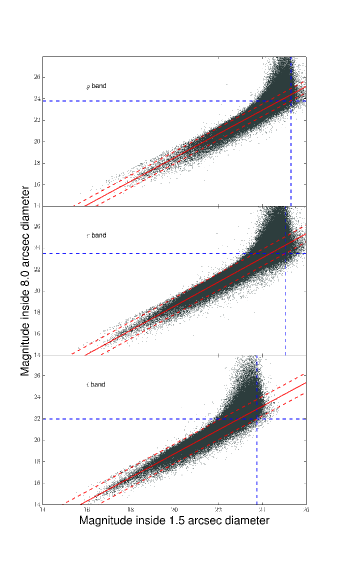
Figure 10: Distribution of the SExtractor magnitude inside a 8.0^′′ diameter as a function of the magnitude inside a detection aperture of 1.5^′′ diameter for $gri$ bands. The horizontal and vertical blue dashed lines indicate the detection and the completeness limits, respectively. The red continuous lines are the linear relation between the magnitude within 8.0^′′ aperture diameter and the magnitude within the detection aperture, minus/plus 1$\sigma$ (red dashed lines).

Fig. 11 shows the distribution of the Kron magnitude, where vertical continuous lines indicate the limit to which the catalogues are complete.

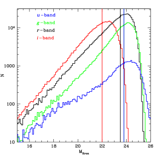
Figure 11: Number counts of galaxies over the observed fields (11, 10, 14, 23, for $u$, $g$, $r$ and $i$, respectively) per 0.1 mag bin. Vertical lines mark the completeness magnitudes. $u$- and $g$-band catalogues have the same completeness magnitude indicated by the blue vertical line.

5 Description of the data base

The $i$-band catalogue is published and it will be regularly updated, through the use of the Virtual Observatory (VO) tools.

The data model of the ShaSS data base is based on the standard Entity-Relationship (ER) paradigm. Its architectural diagram is shown in Fig. 12. Its physical model (band-specific and correlation tables) is instantiated in the logical DataBase Management System (DBMS), based on the open source mySQL data base and on the SVOCat service, a VO software tool developed in the framework of the Spanish Virtual Observatory (http://svo2.cab.inta-csic.es/vocats/SVOCat-doc/) .

The DBMS provides direct access to data through SQL-based queries and VO standard interoperability (i.e. direct table/image exchanging among VO tools, such as Topcat and Aladin). The service is publicly accessible via browser at the address http://shass.na.astro.it .

The Shass data base is also publicly available within the EURO-VO registry framework, under the INAF-DAME Astronomical Archive identification authority (ivo://dame.astro.it/shass-i).

Each object in the data base has a unique primary key (SHASS_ID), which univocally identifies sources. It is composed by a string containing 14 characters, where five characters are for ShaSS and none digits NNNNNNNNN represent the internal object identification number.

The SHASS_ID field represents the primary identifier of an object within the corresponding band table. Whenever an object has a counterpart in different bands, the sequence of different SHASS_IDs for each reference band can be obtained by simple queries to the correlation table in the data base (for instance the corr_tab table in Fig. 12). In this table the fields group and group_size are reported for each band. These indicate the possible presence of a group of objects matching with the single source within 1$\arcsec$ distance. To each group of sources matching with one specific object is assigned a unique integer, recorded in the group field, and the size of each group is recorded in the group_size field. Sources which don’t match any others (singles) have null values in both these fields.

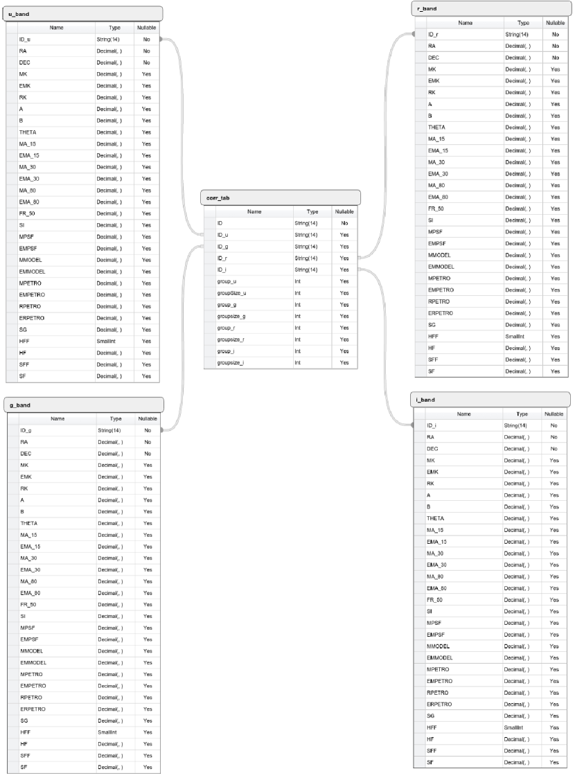
Figure 12: The layout of the ER diagram for the optical ShaSS data base.

In the data base we report the barycenter coordinates in degrees (RAdeg, DECdeg), the geometrical parameters of the ellipse that describes the shape of the objects: semi-major and semi-minor axes, and position angle (A, B, THETA). As an indicator of the area covered by the objects we include the half flux radius (FR₅₀) which corresponds to the radius of the isophote containing half of the total flux. We add the Kron radius (RK) and the Petrosian radius (RPETRO), which are the indicators of size of the Kron and the Petrosian aperture respectively. Both of these radii are expressed in multiples of the semi-major axis.

Among the extracted photometric quantities, we report in the public catalogue three aperture magnitudes (MA) (see Table 7), the Kron magnitude (MK), the magnitude resulting from the PSF fitting (MPSF), the model magnitude obtained from the sum of the spheroid and disk components of the fitting (MMODEL), and the Petrosian magnitude (MPETRO). Magnitudes are not corrected for galactic extinction and we give the relative uncertainties as derived by SExtractor (but see also Sect. 4.2).

Finally we provide the stellarity index from SExtractor (SI) and five flags: the star/galaxy flag (SG), the halo fraction flag (HFF), the halo flag (HF), the spike fraction flag (SFF) and the spike flag (SF).

The star/galaxy flag is fixed according to the star/galaxy separation described in Sect. 3.3. Stars classified according to the SExtractor stellarity index, half flux radius and the spread model have SG=1,2,3 respectively, while those classified through the visual inspection have SG=7. Saturated stars are indicated by SG=9. Sometimes values of the star/galaxy flag SG=4,5 could be present. They indicate stars aligned in a ‘secondary sequence’ visible in a few observed fields in the plots of the half light radius and the $\mu_{max}$ versus the Kron magnitude, respectively. The origin of this secondary sequence is unclear, but it seems a ”random effect” since there is no correlation with observing night, airmass or spatial position of stars, and only constitutes a small number of stars.

As stated in Sect. 3.3, the $r$ band will be used for the classification of sources in the cross-correlated catalogue, while in the $g$ and $i$ single-band catalogues we report the classification independently derived for each band, which is mostly consistent with that of the $r$ band.

The halo and the spike fraction flag indicate the fraction of the object area, defined as the circular area with radius equal to half flux radius, affected by the presence of the halo or the spike of a bright saturated star. Since, as pointed out in Sect. 3.2 the ‘intensity’ of the halo is related to the magnitude of the parent star, flag HF is equal to 100$\times$ i_mag, where i_mag is the star magnitude from the USNO-B1.0 catalogue. Spikes flag values are equal to 1,2 or 3, corresponding to three threshold values of the surface brightness of 20, 20.5 and 21 mag arcsec^-2 of saturated regions (see Sect. 3.2).

A description of the units used for each of the quantities in the data base is reported in Table 7.

We plan to complement the present data base with the catalogues of the $u$, $g$ and $r$ bands and the cross-correlated catalogue following the completion of the observations.

Parameter	Units	Description
ID		ShaSS identification
RAdeg	deg	Right ascension (J2000)
DECdeg	deg	Declination (J2000)
MK	mag	Kron magnitude
EMK	mag	Error on Kron magnitude
RK		Kron radius expressed in multiples of major axis
A	deg	Major axis
B	deg	Minor axis
THETA	deg	Position angle (CCW/x)
MA15	mag	Aperture magnitude inside 1.5 $\arcsec$ diameter
EMA15	mag	Error on aperture magnitude inside 1.5 $\arcsec$ diameter
MA40	mag	Aperture magnitude inside 4.0 $\arcsec$ diameter
EMA40	mag	Error on aperture magnitude inside 4.0 $\arcsec$ diameter
MA80	mag	Aperture magnitude inside 8.0 $\arcsec$ diameter
EMA80	mag	Error on aperture magnitude inside 8.0 $\arcsec$ diameter
FR50	pixel	Radius of the isophote containing half of the total
		flux
SI		SExtractor stellarity index
MPSF	mag	Magnitude resulting from the PSF fitting
EMPSF	mag	Error on magnitude resulting from the PSF fitting
MMODEL	mag	Magnitude resulting from the model of the spheroid
		and disc components
EMMODEL	mag	Error on magnitude resulting from the model of the
		spheroid and disc components
MPETRO	mag	Petrosian magnitude
EMPETRO	mag	Error on Petrosian magnitude
RPETRO		Petrosian radius expressed in multiples of major
		axis
SG		Star Galaxy separation
HFF		Halo fraction flag
HF		Halo flag value
SFF		Spike fraction flag
SF		Spike flag value

Table 7: Parameters reported in the data base.

6 Summary

The ShaSS will map an area of $\sim$23 deg² ($\sim$ 260 h${}_{70}^{-2}$ Mpc² at z=0.048) of the SSC with the principal aim being to quantify the influence of hierarchical mass assembly on galaxy evolution, and to follow this evolution from filaments to cluster cores.

ShaSS will provide the first homogeneous multi-band imaging covering the central region of the supercluster, including optical ($ugri$) and NIR ($K$) imaging acquired with VST and VISTA, which allows accurate multiband photometry to be obtained for the galaxy population down to m*+6 at the supercluster redshift. In particular, the $r$-band images are collected with a median seeing equal to 0.6 arcsec, corresponding to 0.56 kpc h${}^{-1}_{70}$ at z=0.048 and thus enabling the internal properties of supercluster galaxies to be studied and distinguish the impact of the environment on their evolution.

In this article, we described the methodology for producing photometric catalogues. The optical survey is ongoing and the analysis presented in this work is performed on 11, 10, 14 and VST fields out of 23 in $ugr$ bands, nevertheless in all bands the considered subsamples are representative of the final whole sample. The $i$-band imaging is instead complete.

The catalogues are produced using the software SExtractor (Bertin & Arnouts, 1996) in conjuction with PSFEx (Bertin, 2011), and a careful analysis of the software outputs.

We were able to obtain a robust separation between stars and galaxies up to the completeness limit of the optical data, through a progressive approach using: i) the stellarity index (CLASS_STAR); ii) the half-light radius (FLUX_RADIUS) ; iii) the new SExtractor classifier SPREAD_MODEL; iv) the peak of the surface brightness above background ($\mathrm{\mu_{max}}$); v) a final visual inspection for objects classified as galaxies but with CLASS_STAR$>$0.90.

The ShaSS catalogues reach average 5$\sigma$ limiting magnitudes inside a 3$\arcsec$ aperture of $ugri$=[24.4,24.6,24.1,23.3] and a completeness limit of $ugri$=[23.8,23.8,23.5,22.0], which corresponds to $\sim$ m*_r+8.5 at the supercluster redshift. These values correspond to the survey expectations.

The $i$-band catalogue is released to the community through the use of the Virtual Observatory tools. It includes 734 319 sources down to $i$=22.0 over the whole area. The catalogue is 93% complete at this magnitude limit and 34% of the sources are galaxies. The service is publicly accessible via browser at the address http://shass.na.astro.it . The Shass data base is also publicly available within the EURO-VO registry framework, under the INAF-DAME Astronomical Archive identification authority (ivo://dame.astro.it/shass-i) .

References

- Abell, Corwin & Olowin (1989) Abell G. O., Corwin H. G. Jr., Olowin R. P., 1989, ApJS, 70, 1
- Annunziatella et al. (2013) Annunziatella, M., Mercurio, A., Brescia, M., Cavuoti, S., Longo, G, 2013, PASP, 125, 68
- Bardelli et al. (1994) Bardelli S., Zucca E., Vettolani G., Zamorani G., Scaramella R., Collin C. A., MacGillivray H. T., 1994, MNRAS, 267,665
- Bardelli et al. (1998a) Bardelli S., Pisani A., Ramella M., Zucca E., Zamorani G., 1998a, MNRAS, 300, 589
- Bardelli et al. (1998b) Bardelli S., Zucca E., Zamorani G., Vettolani G., Scaramella R., 1998b, MNRAS, 296, 599
- Bardelli et al. (2000) Bardelli S., Zucca E., Zamorani G., Moscardini L., Scaramella R., 2000, MNRAS, 312, 540
- Bardelli, Zucca & Baldi (2001) Bardelli S., Zucca E., Baldi A., 2001, MNRAS, 320, 387
- Bertin & Arnouts (1996) Bertin, E. & Arnouts, S. 1996, A&AS, 117, 393
- Bertin et al. (2002) Bertin et al. 2002: The TERAPIX Pipeline, ASP Conference Series, Vol. 281, 2002 D.A. Bohlender, D. Durand, and T.H. Handley, eds., p. 228
- Bertin (2006) Bertin, 2006, in Gabriel C., Arviset C., Ponz D., Solano E., eds, ASP Conf. Ser. Vol. 351, Automatic Astrometric and Photometric Calibration with SCAMP. Astron. Soc. Pac., San Francisco, p. 112
- Bertin (2011) Bertin, E. 2011, in Evans I. N., Accomazzi A., Mink D. J., Rots A. H., eds, ASP Conf. Ser. Vol. 442, Automated Morphometry with SExtractor and PSFEx, p. 435
- Bouy et al. (2013) Bouy H., Bertin E., Moraux E., Cuillandre J. C., Bouvier J., Barrado D., Solano E., Bayo A., 2013, A&A 554, A101
- Bundy et al. (2012) Bundy, K., Hogg, D., W., Higgs, T. D., Nichol, R. C., Yasuda, N., Masters, K. L., Lang, D., Wake, D. A., 2012, AJ, 144, 188
- Caldwell et al. (2008) Caldwell, J. A. R., McIntosh, D. H.; Rix, H. W. et al. 2008, ApJS, 174, 136
- Christodoulou et al. (2012) Christodoulou L., Eminian C., Loveday J., Norberg P., Baldry I. K., Hurley P. D., Driver S. P., Bamford S. P., Hopkins A. M., Liske J. L. et al., 2012, MNRAS, 425, 1527
- Conselice, Bershady & Jangren (2000) Conselice C. J., Bershady M. A., Jangren A., 2000, ApJ, 529, 886
- De Filippis, Schindler & Erben (2005) De Filippis E., Schindler S., Erben T., 2005, A&A, 444, 387
- Desai et al. (2012) Desai, S., Armstrong, R., Mohr, J. J., et al. 2012, ApJ, 787, 83
- D’Onofrio et al. (2014) D’Onofrio, M., Bindoni, D., Fasano, G., et al. 2014, A&A, 572, 87
- Drinkwater et al. (2004) Drinkwater M. J., Parker Q. A., Proust D., Slezak E., Quintana H., 2004, PASA, 21, 89
- Fabian (1991) Fabian A. C., 1991, MNRAS, 253, L19
- Feindt et al. (2013) Feindt U., Kerschhaggl M., Kowalski M., Aldering G., Antilogus P., Aragon C., Bailey S., Baltay C., et al., 2013, A&A, 560, 90
- Finoguenov et al. (2004) Finoguenov A., Henriksen M. J., Briel U. G., de Plaa J., Kaastra J. S., 2004, ApJ, 611, 811
- Garilli, Maccagni & Andreon (1999) Garilli B., Maccagni D., Andreon S., 1999, A&A, 342, 408
- Grado et al. (2012) Grado A., Capaccioli M., Limatola L., Getman F., 2012, Mem. SAIt Supplement, 19, 362
- Graham & Guzmán (2003) Graham A. W. & Guzmán R., 2003, AJ, 125, 2936
- Haines et al. (2011) Haines C. P., Busarello G., Merluzzi P., Smith R. J., Raychaudhury S., Mercurio A., Smith G. P., 2011, MNRAS, 412, 145
- Häussler et al. (2007) Häussler B., McIntosh D. H., Barden M., Bell E. F., Rix H. W., Borch A., Beckwith S. V. W., Caldwell J. A. R., Heymans C., et al., 2007, ApJS, 172, 615
- Holwerda et al. (2014) Holwerda B. W., Muñoz-Mateos J. C., Comerón S., Meidt S., Sheth K., Laine S. et al., 2014, ApJ, 781, 12
- Hoyos et al. (2011) Hoyos C., den Brok M., Kleijn G. V., 2011, MNRAS, 411, 2439
- Kleiner et al. (2014) Kleiner D., Pimbblet K. A., Owers M. S., Jones D. H., Stephenson A. P., 2014, MNRAS, 439, 2755
- Kocevski, Mullis & Ebeling (2004) Kocevski D. D., Mullis C. R., Ebeling H., ApJ, 2004, 608, 721
- Kron (1980) Kron G., 1980, ApJS, 43, 305
- Kull & Böhringer (1999) Kull A. & Böhringer H., 1999, A&A, 341, 23
- Lotz et al (2008) Lotz J. M., Jonsson P., Cox T. J., Primack J. R., 2008, MNRAS, 391, 1137
- Lotz et al (2011) Lotz J. M.; Jonsson, P., Cox, T. J., Croton D., Primack J. R., Somerville R. S., Stewart K., 2011, ApJ, 742, 103
- Melnick & Quintana (1981) Melnick J., Quintana H., 1981, A&AS, 44, 87
- Mercurio et al. (2006) Mercurio A., Merluzzi P., Haines C. P., Gargiulo A., Krusanova N., Busarello G., La Barbera F., Capaccioli M., Covone G., 2006, MNRAS, 368, 109
- Merluzzi et al. (2010) Merluzzi P., Mercurio A., Haines C. P., Smith, R. J., Busarello G., Lucey J. R., 2010, MNRAS, 402, 753
- Merluzzi et al. (2015) Merluzzi, P., Busarello, G., Haines, C. P., Mercurio, A., Okabe, N., et al., 2015, MNRAS, 446, 803
- Metcalfe, Godwin & Spencer (1987) Metcalfe N., Godwin J. G., Spenser S. D, 1987, MNRAS, 225, 581
- Misgeld, Hilker & Mieske (2009) Misgeld I., Hilker M., Mieske S., 2009, A&A, 496, 683
- Mohr et al. (2012) Mohr, J. J. et al. 2012, The Dark Energy Survey Data Processing and Calibration System, Publicated in Software and Cyberinfrastructure for Astronomy II. Proceedings of the SPIE, Volume 8451, article id. 84510D.
- Muñoz & Loeb (2008) Muñoz J. A., Loeb A., 2008, MNRAS, 391, 1341
- Muñoz-Mateos et al. (2009) Muñoz-Mateos J. C., Gil de Paz A., Zamorano J., Boissier S., and Dale D. A., Pérez-González P. G., Gallego J., Madore B. F., Bendo G., Boselli A.. et al., 2009, ApJ, 703, 1569
- Pearson & Batuski (2013) Pearson D. W. & Batuski D. J., 2013, MNRAS, 436, 796
- Petrosian (1976) Petrosian, V., 1976, ApJL, 209, 1
- Plionis & Valdarnini (1991) Plionis M., Valdarnini R., 1991, MNRAS, 249, 46
- Price et al. (2009) Price J., Phillips S., Huxor A., et al., 2009, MNRAS, 397, 1816
- Proust et al. (2006) Proust D., Quintana H., Carrasco E. R., Reisenegger A., Slezak E., Muriel H., Dünner R., Sodr‘e L. Jr., et al., 2006, A&A, 447, 133
- Quintana et al. (1997) Quintana H., Melnick J., Proust D., Infante L., 1997, A&ASS, 125, 247
- Quintana et al. (1995) Quintana H., Ramirez A., Melnick J., Raychaudhury S., Slezak E., 1995, AJ, 110, 463
- Quintana, Carrasco & Reisenegger (2000) Quintana H., Carrasco E. R., Reisenegger A., 2000, AJ, 120, 511
- Raychaudhury (1989) Raychaudhury S., 1989, Naturem 342, 251
- Raychaudhury et al. (1991) Raychaudhury S., Fabian A. C., Edge A. C., Jones C., Forman W., 1991, MNRAS, 248, 101
- Rix, H. W. et al. (2004) Rix, H.-W., Barden, M., Beckwith, S. V. W., et al. 2004, ApJS, 152, 163
- Rossetti et al. (2005) Rossetti M., Ghizzardi S., Molendi S., Finoguenov A., 2005, A&A, 463, 839
- Scaramella et al. (1989) Scaramella R., Baiesi-Pillastrini G., Chincarini G., Vettolani G., 1989, Nature, 338, 562
- Scarlata et al. (2007) Scarlata C., Carollo C. M., Lilly S., Sargent M. T., Feldmann R., Kampczyk P., et al., 2007, ApJS, 172, 406
- Shapley (1930) Shapley H., 1930, Bull. Harvard Obs., 874, 9
- Smith Castelli et al. (2012) Smith Castelli A. V., Cellone S. A., Faifer F. R., MNRAS, 419, 2472
- Taylor (2006) Taylor, M. B., 2006, ASPC, 351, 666
- Weinmann et al. (2011) Weinmann, S. M.; Lisker T. G., Guo Q., Meyer H. T. & Janz J., 2011, MNRAS, 41, 1197
- Wright et al. (2010) Wright E. L., Eisenhardt P. R. M., Mainzer A. K., Ressler M. E., Cutri R. M., et al., 2010, AJ, 140, 1868