3D adaptive mesh refinement simulations of the gas cloud G2 born within the disks of young stars in the Galactic Center

Abstract

The dusty, ionized gas cloud G2 is currently passing the massive black hole in the Galactic Center at a distance of roughly 2400 Schwarzschild radii. We explore the possibility of a starting point of the cloud within the disks of young stars. We make use of the large amount of new observations in order to put constraints on G2’s origin. Interpreting the observations as a diffuse cloud of gas, we employ three-dimensional hydrodynamical adaptive mesh refinement (AMR) simulations with the PLUTO code and do a detailed comparison with observational data. The simulations presented in this work update our previously obtained results in multiple ways: (1) high resolution three-dimensional hydrodynamical AMR simulations are used, (2) the cloud follows the updated orbit based on the Brackett-$\gamma$ data, (3) a detailed comparison to the observed high-quality position-velocity diagrams and the evolution of the total Brackett-$\gamma$ luminosity is done. We concentrate on two unsolved problems of the diffuse cloud scenario: the unphysical formation epoch only shortly before the first detection and the too steep Brackett-$\gamma$ light curve obtained in simulations, whereas the observations indicate a constant Brackett-$\gamma$ luminosity between 2004 and 2013. For a given atmosphere and cloud mass, we find a consistent model that can explain both, the observed Brackett-$\gamma$ light curve and the position-velocity diagrams of all epochs. Assuming initial pressure equilibrium with the atmosphere, this can be reached for a starting date earlier than roughly 1900, which is close to apo-center and well within the disks of young stars.

1. Introduction

The density distribution and kinematics of objects in the Galactic Center are strongly affected by tidal forces due to the central massive black hole (BH), feedback processes from the cluster of high-mass stars in the direct vicinity of Sgr A*, and the central gas accretion flow. A very prominent example is the recently discovered dusty, ionized gas cloud, G2. It is on an extremely elliptical orbit ($e=0.98$), bringing it as close as 2400 Schwarzschild radii to the central massive BH. The fortuitous detection only a few years before G2’s pericenter passage in early 2014 (during its roughly 400 yr orbital period), enabled us to get a live view of the unfolding tidal disruption. This is best seen in position-velocity diagrams constructed from the Brackett-$\gamma$ emission (but also in other gas tracer lines) detected with the SINFONI (Eisenhauer et al. 2003; Bonnet et al. 2004) instrument at the VLT (Gillessen et al. 2012, 2013a, 2013b; Pfuhl et al. 2015, orbital properties taken from Gillessen et al. 2013b) or OSIRIS (Larkin et al. 2006) at the Keck telescopes (Phifer et al. 2013). The expected rising signature of tidal disruption in total Brackett-$\gamma$ emission has only been seen very close to the nominal time of pericenter passage, following a long plateau ($L_{\mathrm{Br}\gamma}\approx 2\times 10^{-3}\,L_{\odot}$) and hence poses a challenge to available models.

In contrast to the clear disruption signature of the Brackett-$\gamma$ emission, recent L’ band observations (targeting the dust content) using the near-infrared camera NIRC2 and the Keck II laser guide star adaptive optics system (LGSAO, Wizinowich et al. 2006; van Dam et al. 2006) show L’ band diameters of G2 smaller than 260 astronomical units, with a constant magnitude of 14 between 2005 and 2014, even after pericenter passage (Witzel et al. 2014). These observations give important constraints for theoretical models and might help to differentiate between possible models. Dust, however, makes up only a tiny fraction of the total mass of G2. Pfuhl et al. (2015) find a dust mass of roughly $10^{-12}\,M_{\mathrm{\odot}}$. This is consistent with the dust content of a second gas cloud (G1) in the Galactic Centre (Ghez et al. 2005), which evolves on a similar orbit but precedes G2 by roughly 13 years. Due to this very small dust-to-gas ratio, we do not expect the dust component to affect the dynamics and distribution of the gas and neglect its contribution in this article.

Further very recent near-infrared observations of G2 have been reported by Valencia-S. et al. (2015). They find no blue-shifted emission in their February to May 2014 SINFONI data set, but only red-shifted emission and vice versa for the data after May 2014. No significant line broadening of the detected red-shifted Brackett-$\gamma$ line with respect to their 2013 data set was detected. This is interpreted as G2 having passed pericenter in 2014.39 and as an indication for the compactness of the source.

With a SINFONI data set that reaches the highest signal-to-noise ratio of all available data, Pfuhl et al. (2015) come to a different conclusion: with time, the redshifted emission fades and the blue-shifted Brackett-$\gamma$ emission gradually appears and starts to dominate in mid-2014. Evidence is found for a connection of the G2 cloud and the G1 cloud, indicating that a drag force might lead to deviations from a purely Keplerian orbit. This might allow future observations to constrain properties of the hot accretion flow (Pfuhl et al. 2015; McCourt & Madigan 2015). Having reached its pericenter passage roughly 13 years earlier, G1 might give us a preview of what will happen to G2 in the coming years. G1 and the presence of a tail following G2 suggest that they are part of a more extended stream of gas pointing towards Sgr A*.

Many monitoring campaigns of Sgr A* at various wavelengths have been undertaken since the detection of G2 in 2012, but none of them has found unambiguous evidence for a change in the flux density or the activity of Sgr A* which could be attributed to the interaction of G2 gas with the central black hole (Bower et al. 2015; Park et al. 2015, and references therein). After carefully analysing XMM Newton and Chandra observations, Ponti et al. (2015) found that the bright or very bright X-ray flare luminosity of Sgr A* increased by a factor of 2 to 3 between 2013 and 2014. A factor of approximately 9 increase of the bright or very bright flaring rate is reported, which started roughly 6 months after the nominal pericenter passage of G2. Given the not very well known power spectrum of the X-ray flare emission, this could also be caused by the increased monitoring frequency triggered by the G2 detection (Ponti et al. 2015).

As an ideal testbed for the investigation of physical processes in galactic nuclei, this event led to immediate theoretical interest. Burkert et al. (2012) investigated the most important physics involved and possible formation mechanisms for the G2 cloud. Models can be largely separated into two main categories: (1) diffuse gas clouds and (2) gas clouds containing compact sources. The first class could be interpreted as debris from stellar wind interactions (Gillessen et al. 2012; Burkert et al. 2012; Cuadra et al. 2006) or condensations within a stream of gas (Guillochon et al. 2014; Pfuhl et al. 2015). The latter scenario was for example modelled as a photoevaporating protoplanetary / circumstellar disk (Murray-Clay & Loeb 2012; Miralda-Escudé 2012), a mass-losing star (Meyer & Meyer-Hofmeister 2012; Scoville & Burkert 2013; Ballone et al. 2013; De Colle et al. 2014) or the product of a stellar binary merger due to so-called Kozai-Lidov oscillations induced by the central massive black hole (Phifer et al. 2013; Prodan et al. 2015; Witzel et al. 2014).

We will concentrate on the case of a diffuse gas cloud. First two-dimensional hydrodynamical simulations of such a scenario have been presented by Schartmann et al. (2012). Assuming the gas clouds start in pressure equilibrium, have a given gas mass and employing simple test particle simulations, the data necessitated a comparably recent starting point of a Compact Cloud close to the year 1995. But a starting point closer to apocenter is more favorable for several reasons: (1) The cloud spends most of its lifetime in this part of the orbit. (2) It is well within the range of the disk(s) of young stars. The latter are made up of roughly 100 massive O- and Wolf-Rayet stars distributed in a warped clockwise rotating disk ranging from roughly 0.05 to around 0.5 pc (Paumard et al. 2006; Bartko et al. 2009; Lu et al. 2009; Yelda et al. 2014). A fraction of the stars is counter-clockwise rotating and might be associated with a second, inclined disk (e. g.  Paumard et al. 2006). The cloud could then be made up of shocked debris from the interaction of slow winds within these disks of young stars (Burkert et al. 2012). (3) No source of gas has been identified in the vicinity of a starting point around the year 1995. Using the same initial conditions as found in Schartmann et al. (2012), Anninos et al. (2012) ran 3D moving mesh hydrodynamical simulations of the G2 cloud. Similar values were found for the mass transfer rate towards the center. However, no direct comparison to observations was done. The alternative formation scenario which interprets the cloud as the result of mass loss from a compact central source of gas is presented in a companion paper (A. Ballone et al. , 2015, in preparation), together with a comparison of the two basic scenarios.

Despite the large amount of observations and theoretical investigations, the nature of the G2 cloud and its trailing component G2t is still a mystery and many questions remain unanswered, e. g.

1. Is it a pure gas cloud or does it hide a mass-losing source?

2. How did it end up on such a high eccentricity orbit?

3. What is the physical origin of the plateau in the Brackett-$\gamma$ light curve?

4. What is the physical connection between G2, its trailing component G2t, and G1?

The goal of this paper is to build on the knowledge gained so far and set up three-dimensional hydrodynamical simulations to assess the possible origin and fate of the G2 cloud. The most important observational constraints, as well as the updated orbital information, will be taken into account to better constrain a possible initial condition in the framework of the compact cloud scenario and to shed light on the detailed evolution. Most importantly, the 3D AMR simulations allow us to make a much more detailed direct comparison to available data. Such a quantitative analysis was not possible with our preliminary 2D results, wherein the internal cloud structure could not be assessed accurately.

In Sect. 2 we summarize the numerical setup and the parameter settings. The evolution of the gas density of the clouds is presented in Sect. 3. The simulations are compared to observational data in Sect. 4. A critical discussion is presented in Sect. 5 and the conclusions in Sect. 6.

2. Simulation setup

In order to derive the simplest realization of the Compact Cloud scenario, we follow closely the basic setup already used for the simulations described in Schartmann et al. (2012) and Ballone et al. (2013), which we briefly summarize here. The initially spherical cloud evolves in the potential of the massive central BH ($M_{\mathrm{BH}}=4.31\times 10^{6}\,M_{\odot}$) and is embedded into a hot atmosphere. We model the atmosphere following the ADAF realization presented in Yuan et al. (2003):

$$n_{\mathrm{at}}=930\,\mathrm{cm}^{-3}\,f_{\mathrm{hot}}\,\left(\frac{1.4\times 10^{4}R_{\mathrm{S}}}{r}\right)^{\alpha}$$ (1)

$$T_{\mathrm{at}}=1.2\times 10^{8}\,\mathrm{K}\,\left(\frac{1.4\times 10^{4}R_{\mathrm{S}}}{r}\right)^{\beta}$$ (2)

where $n_{\mathrm{at}}$ is the number density distribution and $T_{\mathrm{at}}$ the temperature distribution, both only depending on the distance to the BH $r$. $R_{\mathrm{S}}$ refers to its Schwarzschild radius, the exponents $\alpha$ and $\beta$ are both set to one and $f_{\mathrm{hot}}\approx 1$ is a factor taking the uncertainty of the model into account, which we set to one here. A mean molecular weight of $\mu=0.6139$ has been assumed, typical for a gas with solar metallicity. Following Schartmann et al. (2012), we artificially stabilize the atmosphere, which is unstable to convection. This is done by additionally evolving a tracer field ($0\leq tr\leq 1$), which obeys a simple advection equation and passively follows the fluid:

$$\frac{\partial(\rho\,tr)}{\partial t}+\mathbf{\nabla}\cdot(\rho\,tr\,\mathbf{v})=0,$$ (3)

where $\rho$ is the gas density, $t$ the time and $\mathbf{v}$ the fluid velocity. We initially assign the cloud a value of one for this passive tracer field and the atmosphere zero. This allows us to distinguish between those parts of the atmosphere which have interacted with the cloud ($tr\geq 10^{-4}$) from those which changed due to the atmosphere’s inherent instability ($tr<10^{-4}$). In those cells that fulfil the latter criterion ($tr<10^{-4}$) we reset the density, pressure and velocity to the values expected in hydrostatic equilibrium. For a more detailed description, and a discussion of the consequences for the evolution of the simulations, we refer to Schartmann et al. (2012). Deviating from the work presented there, we update the simulations in two ways: (1) the latest observationally determined best-fit orbital solution for the G2 cloud is used, which is the Brackett-$\gamma$ based orbit as determined by Gillessen et al. (2013b, see their Table 1) and (2) 3D AMR calculations are employed. Three-dimensional simulations have the main advantage that they allow for a detailed comparison with the observed position-velocity diagrams as well as the time evolution of the Brackett-$\gamma$ emission. With our previous 2D simulations, no quantitative comparison was possible. The new 3D simulations allow for the best use of the available data in constraining the initial conditions for the cloud. Providing such a best-fit hydrodynamical model for G2 in the framework of the Compact Cloud Scenario is the main objective of this publication.

A Cartesian coordinate system spanning a volume of $-2.7\times 10^{17}$ cm to $3.7\times 10^{16}$ cm in $x$-direction, $-7.8\times 10^{16}$ cm to $7.8\times 10^{16}$ cm in $y$-direction and $-3.9\times 10^{16}$ cm to $3.9\times 10^{16}$ cm in $z$-direction is used. The orbital plane is given by the x-y plane. Using up to six levels of refinement, a spatial resolution of $3.8\times 10^{13}$cm is reached. The spherical cloud is initially in pressure equilibrium on a clockwise orbit within the $x$-$y$-plane with the major axis along the $x$-axis and the pericenter of the orbit on the positive $x$-axis. The BH is located at the origin of our coordinate system. Various starting positions along the observed orbit (Gillessen et al. 2013b) are tested and the implications of a resolution study are discussed, see Table 1 for an overview of all simulations. The mass of the cloud is fixed to the value estimated from observations ($M_{\mathrm{cloud}}=1.7\times 10^{28}\,$g) in Gillessen et al. (2012).

The simulations make use of the PLUTO code (v4.0, Mignone et al. 2007, 2012) to integrate the hydrodynamical equations, for which the two-shock Riemann solver is chosen together with a parabolic interpolation and the second-order Runge-Kutta time integration scheme. All boundaries are set to the hydrostatic equilibrium values expected for the hot atmosphere. This includes a sphere with a radius of $10^{15}$ cm surrounding the central massive BH. Gas is allowed to flow from the computational domain into this central cavity, but not vice versa. Only the equations of hydrodynamics are taken into account. We exclude thermal conduction, magnetic fields or any kind of feedback from the central source. The AMR technique is used to enable efficient calculations of the cloud evolution in 3D, where we refine according to the second derivative of the density field. Apart from this, the same numerical schemes are applied as described in Schartmann et al. (2012).

Table 1Parameters of the hydrodynamical simulations.

name	$\tau_{0}$	$\rho_{\mathrm{cloud}}$	$R_{\mathrm{cloud}}$	$x_{\mathrm{ini}}$	$y_{\mathrm{ini}}$	$v^{x}_{\mathrm{ini}}$	$v^{y}_{\mathrm{ini}}$	$\Delta x$
	yr AD	$10^{-19}\,\mathrm{g}\,\mathrm{cm}^{-3}$	$10^{15}\,\mathrm{cm}$	$10^{16}\,\mathrm{cm}$	$10^{16}\,\mathrm{cm}$	$\mathrm{km}\,\mathrm{s}^{-1}$	$\mathrm{km}\,\mathrm{s}^{-1}$	$10^{13}\,\mathrm{cm}$
1818L	$1817.9$	0.53	4.24	-25.80	0.00	0.00	72.64	15.17
1850L	$1850.0$	0.55	4.19	-25.36	0.73	88.02	71.37	15.17
1850M	$1850.0$	0.55	4.19	-25.36	0.73	88.02	71.37	7.59
1850H	$1850.0$	0.55	4.19	-25.36	0.73	88.02	71.37	3.79
1870L	$1870.0$	0.58	4.11	-24.62	1.18	145.58	69.17	15.17
1880L	$1880.0$	0.61	4.06	-24.11	1.39	175.84	67.57	15.17
1880M	$1880.0$	0.61	4.06	-24.11	1.39	175.84	67.57	7.59
1880H	$1880.0$	0.61	4.06	-24.11	1.39	175.84	67.57	3.79
1890L	$1890.0$	0.64	3.99	-23.51	1.60	207.47	65.58	15.17
1900L	$1900.0$	0.68	3.91	-22.80	1.80	240.85	63.12	15.17
1920L	$1920.0$	0.79	3.72	-21.05	2.18	314.84	56.36	15.17
1971L	$1971.0$	1.75	2.85	-13.96	2.82	604.22	12.24	15.17
1995L	$1995.0$	4.62	2.06	-8.34	2.67	928.82	-72.12	15.17

3. Evolution of the density distribution

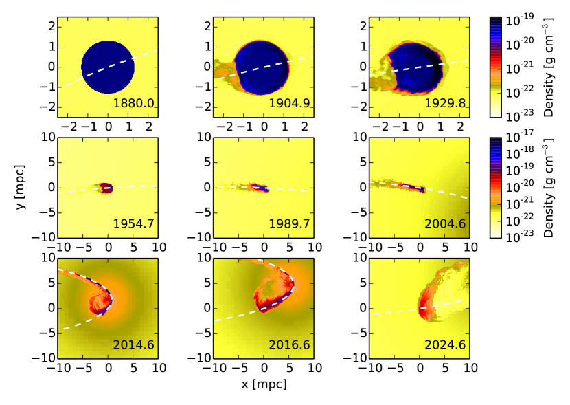
The general evolution of the density distributions of the Compact Cloud models was already discussed in great detail in Schartmann et al. (2012). The 3D simulations show qualitatively the same behavior. This is shown for model 1880M (see Table 1) in Fig. 1. We will refer to the latter simulation as the standard model throughout the paper. The clouds start with spherical shape and in pressure equilibrium with the atmosphere. Moving closer to Sgr A*, the surrounding density, temperature, and therefore also the pressure increase steeply, leading to a slight spherical contraction of the cloud (first row in Fig. 1). The dominant effect during the evolution close to pericenter is the tidal interaction with the BH, stretching the cloud in direction towards the BH and squeezing it perpendicular to it (Fig. 1, middle row). Ram pressure interaction with the dense atmosphere surrounding the BH leads to a compression of the front part of the cloud. Additionally, the cloud experiences fluid instabilities when interacting with the atmosphere, dominated by gas stripping initiated by the Kelvin-Helmholtz instability. The last row in Fig. 1 shows the currently ongoing pericenter passage and the late time evolution. The interaction with the atmosphere then leads to the formation of a nozzle-like structure feeding gas towards the central massive BH (Fig. 1, lower right panel). A starting date as early as applied in some of the simulations presented here will slightly change the orbit. This is because of a slight decrease of the kinetic energy and angular momentum redistribution due to the interaction with the ambient atmosphere as well as the ram pressure compression of the front part of the cloud (see discussion in Burkert et al. 2012). The biggest problem for a direct comparison with the recent observations is that the positions are slightly shifted. The fitting of a new orbit taking hydrodynamical effects into account is beyond the scope of this publication, but we account for this effect by allowing for a time shift of our simulations relative to the observations. In future, more detailed investigations of this shift in orbital parameters compared to the purely ballistic orbit could provide valuable information on the structure of the surrounding diffuse gas component.

Figure 1.— Characteristic time snapshots of the evolution of the cloud in the standard model 1880M. Shown are cuts through the 3D density distribution within the orbital plane, centered on the nominal position along the orbit. Indicated is the simulation time of the respective snapshots. This time might be different with respect to the time when G2 is observed at that position due to the time shift discussed in Sect. 4.2. The white dashed line refers to the nominal orbit. The cloud is first compressed due to the increasing pressure of the atmosphere with decreasing distance from the black hole (upper row), then suffers from hydrodynamical instabilities at its boundary (middle row) and gets tidally stretched along the orbit and partly accreted towards the central BH (lower row).

4. Comparison to observations

We describe G2’s appearance on the sky – based on our simulations – as observable with the SINFONI instrument in Sect. 4.1. The comparison with the observations is split into two parts: (1) position-velocity diagrams enable us to constrain the cloud’s size evolution and morphology and (2) the total Brackett-$\gamma$ light curve gives additional constraints for our models.

4.1. G2’s appearance on the sky

Figure 2.— Simulated, normalized Brackett-$\gamma$ emission for the standard model 1880M projected on the sky and convolved with Gaussian distributions according to the instrumental FWHM values. Overlaid are white contours where half the maximum of the fitted 2D Gaussian is reached. Annotated is the simulation time. The cloud starts only marginally resolved and spherically symmetric. Moving closer to pericenter, it elongates in direction of motion and after pericenter in perpendicular direction.

In order to be able to directly compare our simulations to the observed Brackett-$\gamma$ emission maps and position-velocity diagrams, we transfer our AMR data into a 3D data cube spanned by right ascension (RA), declination (DEC) and line of sight velocity ($v_{\mathrm{los}}$) with the same pixel sizes (12.5 mas in coordinate direction and 69.6 km s^-1 in velocity direction) as the one obtained from the SINFONI observations. This projection makes use of the orbital elements as derived by Gillessen et al. (2013b, Table 1, right column) for the Brackett-$\gamma$ orbit. The cells of the cube are filled with the respective total luminosity in the Brackett-$\gamma$ line as derived with the formalism given in Ballone et al. (2013). In brief, we estimate the Brackett-$\gamma$ emissivity, following Case B recombination theory:

$$j_{\mathrm{Br}\gamma}=3.44\times 10^{-27}\,\left(\frac{T}{10^{4}\,\mathrm{K}}\right)^{-1.09}\,n_{\mathrm{p}}\,n_{\mathrm{e}}\,\mathrm{erg\,s^{-1}\,cm^{3}},$$ (4)

where $T$ is the gas temperature and $n_{\mathrm{p}}$ and $n_{\mathrm{e}}$ are the proton and electron number densities within the respective grid cell. Eq. 4 is the result of a fit to the recombination coefficients (for $T=5,000$, 10,000 and 20,000 K) as presented in Osterbrock & Ferland (2006), which is in reasonable agreement with the approximations found in Ferland (1980) and Hamann & Ferland (1999). To obtain the total Brackett-$\gamma$ luminosity within the mock SINFONI cube, we integrate over the volume of the corresponding region of the simulation data, wherever our cloud tracer value is above $10^{-4}$. Hence, the temperature change due to mixing with the hot surrounding atmosphere is taken into account. The resulting cube is then smeared out by applying a luminosity conserving Gaussian convolution with a full width at half maximum (FWHM) size of 81 mas in coordinate directions and 120 km s^-1 along the velocity axis, mimicking the characteristics of the SINFONI observations. This convolution makes the PV diagrams shown in the following independent of simulation resolution.

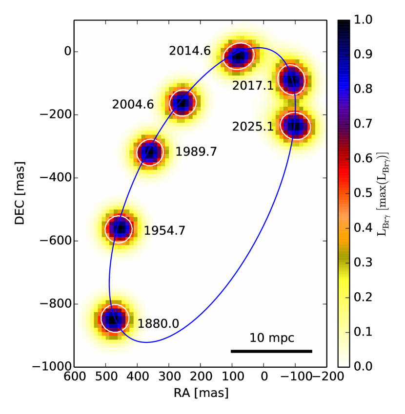
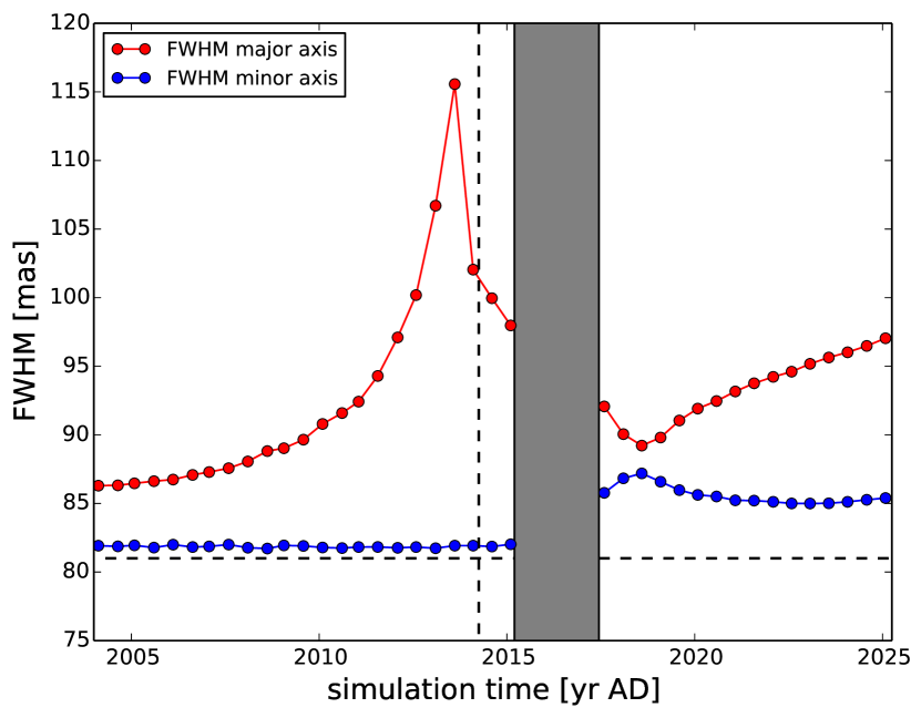
The resulting projection on the sky (neglecting foreground extinction) is shown in Fig. 2. We fit 2D Gaussians and overlay the contour at half the maximum of the fitted 2D Gaussian for various timesteps as indicated. The FWHM of the fitted Gaussian distributions along the major and minor axis are shown as a function of time in Fig. 3. The cloud stays spherically symmetric until roughly 1920, when it begins to slightly elongate in direction of motion until shortly after pericenter. The reason for the elongation is the decrease of the minor axis towards the instrumental FWHM of 81 mas from roughly 1920 onwards due to the compression from the increasing atmospheric pressure, and later on, due to tidal compression. The FWHM of the major axis decreases only slightly, as ram pressure and atmospheric compression are partly balanced by tidal stretching. From roughly 2000 onward the tidal forces dominate and stretch the cloud significantly. Close to pericenter a FWHM of roughly 115 mas is reached. At this time the front part of the cloud already starts to wrap around the BH. The tidal disruption is faster closer to the BH and the cloud gas also heats up significantly during pericenter passage (see discussion in Sect. 5). These processes lead to a decrease of the fitted FWHM close to pericenter and the maximum of the Brackett-$\gamma$ emission also shifts backwards within the cloud. During and shortly after pericenter passage, the cloud is not well described by a Gaussian distribution (given by the gray-shaded interval in Fig. 3). At the latest snapshots shown in Fig. 2 after the cloud has started to contract again in direction of motion (see Fig. 1), the elongation changes to be perpendicular to the orbital motion. This is similar to the morphology of the blue channel image representing the Brackett-$\gamma$ emission of G1 in Fig. 6 of Pfuhl et al. 2015. Due to the uncertainties discussed earlier, however, the evolution past pericenter is only partly physical in our simulations and has to be analyzed with care, especially because of the steep drop of the Brackett-$\gamma$ luminosity (Sect. 4.3). Even models with a very wide-stretched gas density distribution close to pericenter (e. g. model 1880M, see Fig. 1) result in only moderately extended Gaussian FWHM following our sky projection procedure. Until the end of our simulation (at around 2025), we measure FWHM values similar to the ones before pericenter. Therefore, our simulated cloud would be interpreted as a rather compact object.

Figure 3.— Evolution of the full width at half maximum of the normalized Brackett-$\gamma$ emission projected on the sky for the standard model 1880M (compare to Fig. 2). The black dashed horizontal line denotes the instrumental FWHM of 81 mas, with which the simulations were convolved. The vertical dashed line marks the position of nominal pericenter passage. Gray-shaded is the time interval in which the Brackett-$\gamma$ emission of the cloud significantly deviates from a Gaussian shape. No time shift is applied to the simulation data in this figure. Clearly visible is the tidal stretching of the cloud before pericenter.

4.2. Position-velocity diagrams

Position-velocity (PV) diagrams give us the possibility to gain observational insight into the dynamical evolution and the tidal disruption of the gas cloud (see Fig. 4, left panels). To this end, we derive mock SINFONI data cubes from our simulation data (see Sect. 4.1) and extract the PV diagrams along the orbit from the data cube in a similar way as done for the observations in order to allow for a direct comparison: To derive the relative position along the orbit for all simulation grid points, we first project them on the orbit. In a further step, we extract the standard deviation $\sigma$ of the fluctuation spectrum of the observed PV diagrams within a region unaffected by the cloud or streamer. In order to allow for a better comparison by eye, this is then used to overlay the according white noise onto the simulated PV diagram. For the numerical calculation of the best match, the simulated PV diagrams without noise are used. Both observed and simulated PV diagrams are then normalized to the peak Brackett-$\gamma$ luminosity of all pixels. This enables us to separate the constraints on the size and stretching of the cloud from the total emission, and thereby significantly simplifies finding a best-fit model. The simulated PV diagrams calculated in this way are shown in the middle column of Fig. 4. To allow for a quantitative evaluation of the comparison with observations, we calculate normalized residuals in a rectangular region with $21\times 21$ pixels surrounding the maximum within the G2 cloud in the observed PV diagram in the following way:

$$\delta^{2}(v_{\mathrm{los}},x_{\mathrm{orb}})=\left(\frac{PV_{\mathrm{obs}}-PV_{\mathrm{sim}}}{\sigma}\right)^{2},$$ (5)

where all arrays are functions of the line of sight velocity ($v_{\mathrm{los}}$) and the relative position along the orbit ($x_{\mathrm{orb}}$) and $PV_{\mathrm{sim}}$ refers to the normalized simulated PV diagram without noise. The resulting $\delta^{2}$-arrays are shown in the right hand panels of Fig. 4. Summing up of the two-dimensional $\delta^{2}$ array leads us to the $\chi_{\mathrm{r}}^{2}$ value which we use to characterize the quality of the match:

$$\chi_{\mathrm{r}}^{2}=\frac{1}{N-1}\,\sqrt{\sum\delta^{2}},$$ (6)

where $N=421$ is the total number of pixels of the $\delta^{2}$ array. The closer $\chi_{\mathrm{r}}^{2}$ to one, the better the match with the data. In this metric, a model with a PV diagram equal to zero everywhere results in $\chi_{\mathrm{r}}^{2}$ values of 4.37 for the 2008 observation, 7.93 for 2010, 13.25 for 2011, 14.53 for 2012 and 12.78 for 2013. This procedure is repeated for all simulation snapshots with a time interval of typically 0.5 yr, which we compare to all observational epochs in this work. For a more detailed description of the construction of PV diagrams from our AMR data we refer to A. Ballone et al. (2015, in preparation).

4.2.1 The standard model

Figure 4.— Comparison of observed (left panels) and best-fit simulated (middle panels) position-velocity diagrams of our standard model 1880M for several observational epochs as indicated in the left panels. Indicated in the middle panel is the simulation time. The simulation data has been convolved with a Gaussian and noise has been added (see Sect. 4.2). The right hand panels show the normalized residuals $\delta^{2}$ (given in Eq. 5). These are based on the simulated PV diagrams without added noise. The resulting $\chi_{\mathrm{r}}^{2}$ values are given in the lower right corners. All diagrams are normalized to their respective maxima. The observational data is adapted from Gillessen et al. (2012, 2013a, 2013b) and Pfuhl et al. (2015). A good match with observations is found, except for the high velocity gas at small distances from pericenter in 2013.

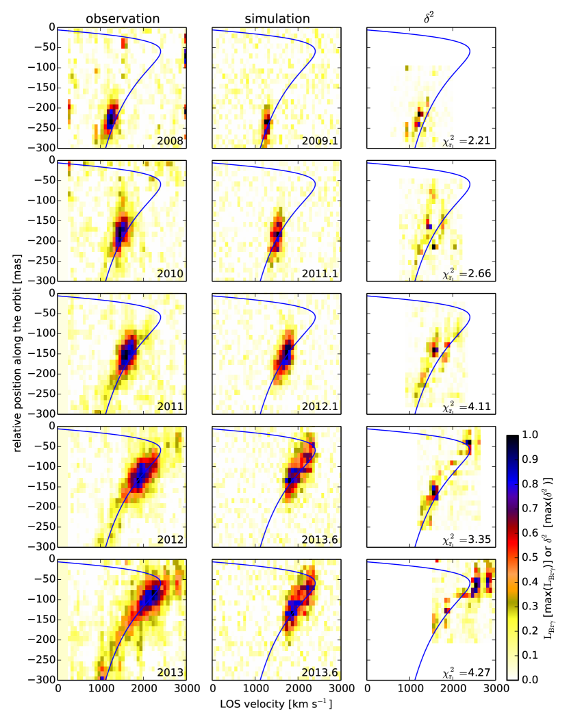
The result of this procedure is summarized in Fig.  4 for the standard model. For selected observation epochs (various rows), the left hand side panel displays the observed PV diagram, the middle one is the best-fitting simulation snapshot and the right hand side panel displays the normalized residual $\delta^{2}$ array. The years 2004 and 2006 have too low signal-to-noise ratios in order to allow for a meaningful comparison and are omitted here. The best match is not obtained at the simulation time of the observed epoch, but with roughly one year delay. The exception of the 2013 epoch will be discussed in more detail below and in Sect. 4.2.2. This is a small effect given the orbital time of roughly $391\pm 66$ years, but needs to be taken into account for a thorough comparison with observations. The reason for this time shift is the hydrodynamical interaction of the cloud with the hot atmosphere. Due to the early starting time of the simulation, the ram pressure interaction has accumulated and becomes noticeable in form of a deceleration of the cloud, which thereby ends up on a slightly different orbit. This change in orbital evolution is approximated by the introduction of the mentioned time shift. The 2013 epoch is a special case, as by then, the front part of the cloud was already in the process of pericenter passage. Due to the tidally stretched appearance of the cloud, the pericenter passage takes up to several years when taking low density gas into account. Given the remaining problems in our simulations during pericenter passage (see discussion in Sect. 5), we decided to restrict the quantitative part of our analysis to the pre pericenter evolution. The middle panels of the 2012 and 2013 epochs also demonstrate the influence of the added noise to the appearance of the cloud in the PV diagrams, as they are showing the same simulation snapshots.

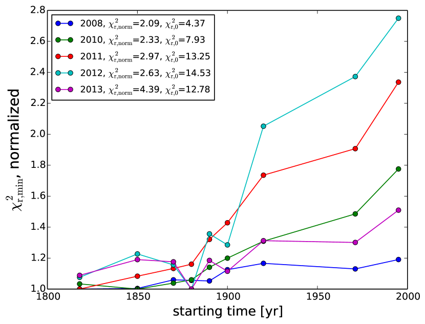
4.2.2 Starting time study

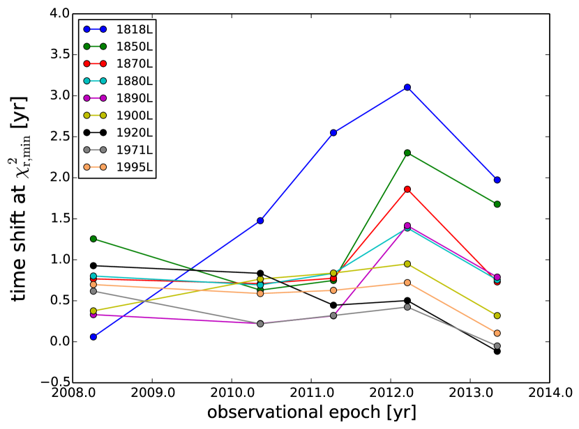
Fig. 5 displays a summary of this analysis for a number of simulations (see Table 1) in which we change the starting time of the cloud in pressure equilibrium for the five observing epochs 2008, 2010, 2011, 2012 and 2013. The $\chi_{\mathrm{r}}^{2}$ parameters shown are the minima after comparing all simulation snapshots with the respective observation. Each curve corresponding to an observational epoch is normalised to its minimum value, which are given in the legend of the plot. Absolute $\chi_{\mathrm{r}}^{2}$ are given for some simulations in Table 2. The different slopes of the curves for various observational epochs relate to the increasing offset of the observed PV diagram from the nominal orbit, which can not be accounted for in the simulations and the different noise levels. The best constraint for our simulations is given by the 2011 and 2012 epochs (showing the steepest curves) and almost no constraint can be derived from the 2008 epoch (flat distribution). The resulting time shifts with respect to the simulation time are up to 3 years and tend to increase towards later observing epochs (Fig. 6). Given that a range of 80 years in starting time lead to a good comparison with the data (given by the plateau in Fig. 5 for starting times earlier than approximately 1900), it is a small effect. This shows that deviations from a ballistic orbit are minor in this evolutionary stage. The increase towards later observing epochs might be evidence for a too strong interaction of the cloud with the atmosphere, which could either be caused by a too large cross section of the cloud in this evolutionary phase or necessitate a change of the structure of the assumed atmosphere in the corresponding radius regime. However, part of the increase could also be related to different data quality of the epochs, the uncertainty of the orbit and the (partly artificial) mixing of cloud material with the atmosphere (see Sect. 4.3.2). For the 2013 observation epoch the time shifts decrease again, which is consistent with the observational finding that part of the cloud has already passed pericenter at that time (Gillessen et al. 2013b). As a consequence, the best comparison with the observations in 2012 and 2013 is reached for the same simulation snapshot (2013.6), as can be seen in the last two rows of Fig. 4.

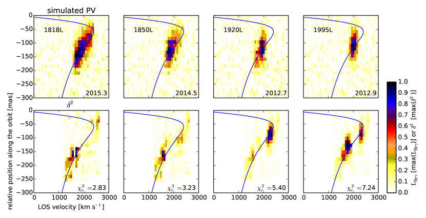
Fig. 7 shows the comparison of the position-velocity diagrams of a subset of the simulations for the observing epoch of 2012. The upper row shows the simulated PV diagrams including noise and the lower row depicts the corresponding normalized residuals $\delta^{2}$. The residuals indicate that the models with the late starting times (1920L and 1995L in this example) underestimate the size of the cloud and a good match is reached for the early starting times. This is also quantified in Table 2. E. g. for the 2012 observation, the standard model reaches a factor of 2.2 lower $\chi_{\mathrm{r}}^{2}$ value compared to the 1995L model and a factor of 4.3 lower compared to a PV diagram with zeros everywhere. Altogether, this clearly shows that an early starting time at around the year 1900 or earlier is favoured by this detailed comparison to observations. The reason for this is the tidal stretching which needs to fully unfold in the simulations and finally leads to the observed structure of the cloud. The plateau in Fig. 5 at early starting times is caused by the slow evolution of the cloud close to apo center.

Figure 5.— Normalized $\chi_{\mathrm{r,min}}^{2}$-values (see Eq. 6) for all starting times of the simulations, normalized to their respective minima (as given in the legend by $\chi_{\mathrm{r,norm}}^{2}$) and color-coded according to the observation epoch. The low resolution simulations have been used for this analysis. $\chi_{\mathrm{r,0}}^{2}$ corresponds to a PV diagram filled with zeros. Compare to Fig. 6 for the applied time shifts and Table 2 for absolute values of $\chi_{\mathrm{r}}^{2}$. This indicates that the closest match with observed PV diagrams is reached for starting times close to or earlier than 1900.

Table 2Resulting $\chi_{\mathrm{r}}^{2}$ values (Eq. 6) for the comparison of simulated and observed PV diagrams for selected models.

name	2008	2010	2011	2012	2013
1880M	2.21	2.66	4.11	3.35	4.27
1995L	2.49	4.13	6.94	7.24	6.62
PV=0	4.37	7.93	13.25	14.53	12.78

Figure 6.— Resulting time shifts from the comparison of simulated to observed PV diagrams as described in Sect. 4.2. Compare to Fig. 5 and Table 2 for the corresponding $\chi_{\mathrm{r,min}}^{2}$ parameters. The tentative increase towards later epochs is due to the interaction with the atmosphere. The drop for the 2013 epoch is caused by the fact that part of the cloud has passed pericenter and we are only comparing red-shifted emission.

Figure 7.— Comparison of simulated position-velocity diagrams (including noise extracted from the observed ones) with the observations in 2012 for simulations with various starting times as annotated (upper row). The snapshot simulation time is given in the lower right corner. The lower row shows the corresponding normalized residuals arrays $\delta^{2}$ (see description in Sect. 4.2). The blue curve denotes the nominal orbit of G2 as derived from observations in Gillessen et al. (2013b). The plot clearly demonstrates that an earlier starting point results in a better match with observations.

4.3. The Brackett-$\gamma$ luminosity evolution

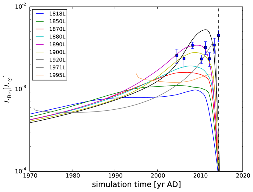
In order to derive the time evolution of the total Brackett-$\gamma$ emission (see Fig. 8), we use Eq. 4 and the formalism described in Sect. 4.1. Because of the homogeneous density and temperature distribution of the initial clouds and the gradient in atmospheric pressure, only the central part of the cloud is in pressure equilibrium and the very first phase of the evolution is given by this slight pressure adjustment. Given the power-law assumption for the atmospheric profiles, this radial pressure inequality is stronger when starting the cloud closer to Sgr A*. This is directly visible in the initial drop of the Brackett-$\gamma$ luminosity close to the starting point of the simulations (Fig. 8) when comparing the 1995 light curve with the 1971 one.

Figure 8.— Total Brackett-$\gamma$ luminosity evolution for simulations with various starting times as indicated in the legend. Overplotted as blue symbols with error bars are the observational data from Gillessen et al. (2012, 2013a, 2013b) and Pfuhl et al. (2015). No time shift is applied to the simulation data in this figure. The early rising signature due to atmospheric compression is followed by a plateau due to mixing with the atmosphere and a steep drop, which is caused by the strong expansion of the cloud post pericenter. The resolution dependence is shown in Fig. 10.

4.3.1 Atmospheric compression

The longest phase of the evolution of the light curve is given by compression due to the pressure increase when moving towards the central part of the atmosphere. The low sound speed of approximately $c_{\mathrm{s}}=10\,\mathrm{km}\,\mathrm{s}^{-1}$ within the cloud with an initial sound crossing time of the order of 50 to 100 years for the simulations shown here (see Table 1) leads to a slowly inward growing spherical density enhancement and a slow compression of the cloud (see Fig. 1, upper row). Despite having a constant mass and lower density at the beginning, models with an earlier starting time end up with a higher Brackett-$\gamma$ luminosity compared to the later starting simulations. The reason is the formation of this dense, outer shell due to this atmospheric pressure confinement and the scaling of the Brackett-$\gamma$ emissivity with $\rho^{2}$ (Eq. 4). This behaviour is visible in between roughly 1950 and 1970 and hence does not show up in Fig. 8.

4.3.2 Mixing plateau

Figure 9.— Histograms of the Brackett-$\gamma$ emission as a function of the density and temperature for a starting time of the cloud in 1880. Shown are models 1880L (upper row), 1880M (middle row) and 1880H (lower row). The simulation name is made up of the starting time and a letter indicating the resolution, see Tab. 1. The histograms demonstrate the effect of the resolution and mixing of the simulations on the Brackett-$\gamma$ emission.

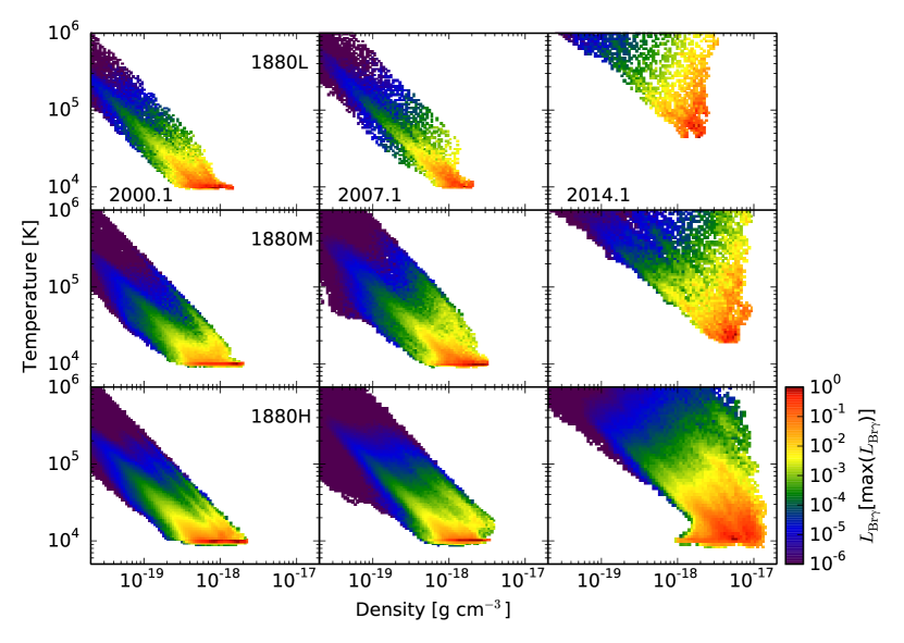
The trend is only broken due to the limited resolution of the simulations, which enhances the mixing with the hot atmosphere and stalls further compression due to the atmospheric confinement. The mixing is partly physical and partly of numerical origin and has two effects. It (1) lowers the density of the cloud and (2) leads to an increase of the temperature, as is seen in the phase diagrams for the Brackett-$\gamma$ emission presented in Fig. 9. In these diagrams for the 1880 models the cloud starts in a single point with a temperature of $10^{4}$ K and a density of $6.1\times 10^{-20}\,\mathrm{g\,cm}^{-3}$. The atmospheric compression and the tidal evolution only change the density structure in these isothermal simulations, visible in the horizontal stretching of the red linear feature. The mixing with the atmosphere at the boundary of the cloud lowers the contribution of cloud material to the total density of the respective grid cells. The increasing contribution of the atmospheric gas heats up the cells. This dilution increases with distance from the cloud and leads to the apparent correlation of density and temperature in Fig.  9. Both effects lower the Brackett-$\gamma$ emission in our formalism (see Eq. 4) and finally lead to the partial dissolution of the cloud.

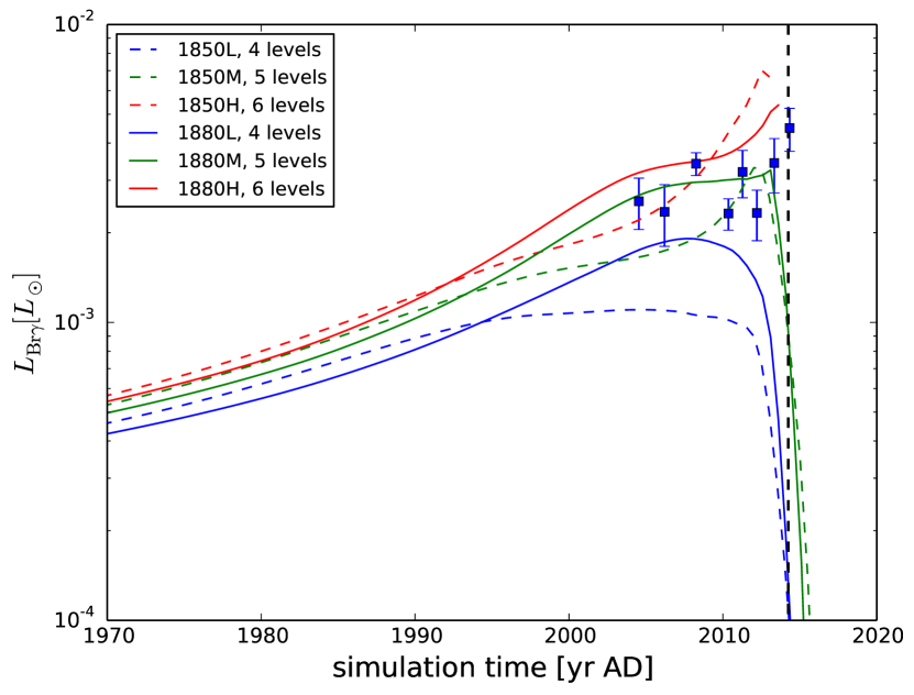
The effect of resolution on the light curves is shown in Fig. 10 for the 1850 and 1880 models. The lower the resolution, the earlier the curves level off, as the numerical mixing is stronger due to the coarser grid. The visible correlation with the starting time of the simulation results from the longer time period in which they are able to mix with the atmosphere. Many of the simulations show a well-defined, constant luminosity “mixing plateau”, which roughly follows the phase dominated by pressure confinement.

Figure 10.— Brackett-$\gamma$ luminosity evolution for two resolution studies. Overplotted as blue symbols with error bars are the observational data from Gillessen et al. (2012, 2013a, 2013b) and Pfuhl et al. (2015). No full convergence is reached. Only very high resolution simulations are able to resolve the steep rise towards pericenter which is caused by tidal compression.

4.3.3 Tidal compression

The steep increase of the light curves later on is caused by tidal compression. This increase is only present in light curves of well resolved simulations. Under the assumption of hydrostatic equilibrium between tidal forces and thermal pressure within the cloud a Gaussian density distribution perpendicular to the momentum direction results. Its full width at half maximum is given by

$$\mathrm{FWHM}=2\,\sqrt{2\,\ln{2}}\,\sqrt{\frac{r^{3}\,k_{\mathrm{B}}\,T}{G\,M_{\mathrm{BH}}\,\mu\,m_{\mathrm{u}}}},$$ (7)

where $r$ is the distance to Sgr A*, $k_{\mathrm{B}}$ is the Boltzmann constant, $T$ is the temperature within the cloud, $M_{\mathrm{BH}}$ is the mass of the central BH and $\mu\,m_{\mathrm{u}}$ is the mean molecular weight (in grams) of the gas in the cloud.

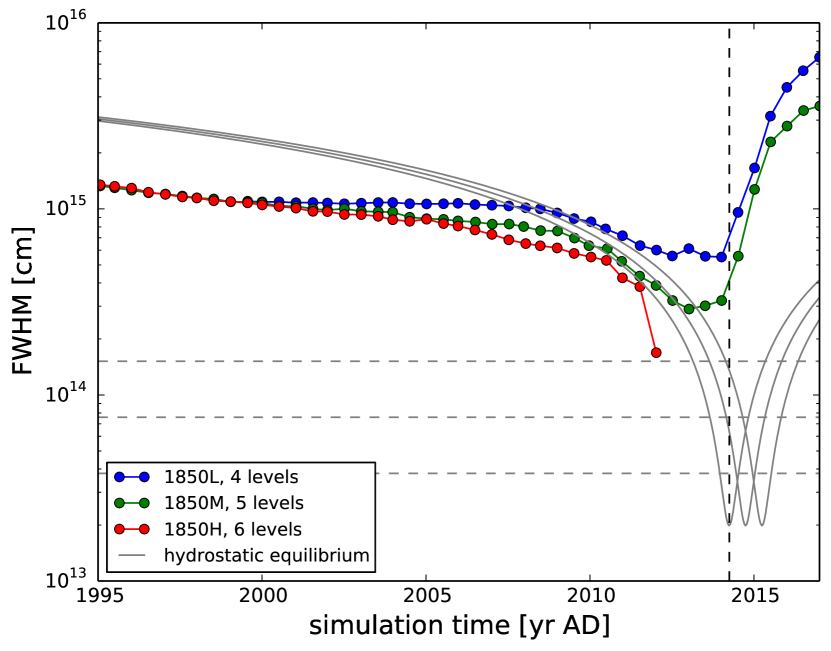
To understand the late time behaviour better, we extract the density distribution of the cloud perpendicular to the momentum vector and fit Gaussian distributions. Fig. 11 shows the full width at half maximum of an average Gaussian distribution derived at ten equidistant positions on the orbit with a maximum separation of $2.5\times 10^{14}\,$cm along the orbit with respect to the nominal position of G2 at the respective time. An average is taken as the cloud has developed substructures at that time. At the beginning of the simulations and for the longest part of their evolution, the pressure forces due to the surrounding atmosphere dominate over the tidal compressive forces, leading to FWHM values below the ones derived for the simple analytic tidal disruption model. This implies that only extremely high resolution simulations are able to resolve the expected Gaussian density distribution close to pericenter passage.

Figure 11.— FWHM of a Gaussian fit to the cloud density distribution perpendicular to the velocity vector at the position of the nominal orbit and surrounding it for simulations 1850L (blue), 1850M (green) and 1850H (red). The simulation name is made up of the starting time and a letter indicating the resolution, see Tab. 1. The gray curves refer to a simple model where hydrostatic equilibrium with the tidal compressional forces is assumed. The dashed horizontal lines show the resolution of the simulations and the dashed vertical line denotes the nominal pericenter. The limited resolution of the simulations prevents stronger compression and only the high resolution simulations result in a reasonable adaptation of the analytic model. Shown here are the results for a starting time in 1850, as this resolution effect is more pronounced for an earlier starting time.

4.3.4 Post pericenter evolution

After G2’s pericenter passage, all our simulations predict a steep drop of the Brackett-$\gamma$ luminosity (Fig. 8), which is caused by heating due to mixing with the atmosphere and the fast expansion of the cloud, which is only partially physical. This is in tension with the relatively high level of blue-shifted Brackett-$\gamma$ flux observed in the latest epoch (Pfuhl et al. 2015). The post-pericenter evolution is strongly dependent on the assumed physics and a more detailed investigation will be necessary.

4.4. Possible interpretations

The best comparison of the PV-diagrams with the observations was reached for a starting time in 1900 and earlier. The PV diagrams give us the best constraints for our models, independent of the resolution. A similar conclusion concerning the best starting time results from the comparison with the Brackett-$\gamma$ luminosity evolution shown here. However, the luminosity evolution is not fully converged with resolution for the simulations presented here and, therefore, has only little constraining power. In addition, the following needs to be considered:

1. Due to the sparse observational coverage, our choice of the atmosphere should be considered an assumption. E. g. changing the slope or the normalisation of the density distribution will change both the comparison to the PV diagrams and the evolution of the light curve.

2. The cloud mass is fixed to the observationally estimated value. Changing the initial cloud mass affects the size and luminosity evolution.

3. A dynamically relevant magnetic field strength has recently been found in the Galactic Center region by Eatough et al. (2013). Depending on the exact strengths and morphologies of the field lines, this changes the mixing behaviour (e. g.  McCourt et al. 2015) and additional, counterbalancing pressure forces might lead to an “arresting” of the cloud (Shcherbakov 2014; Schartmann et al. 2012). Depending on the strength, the process might be able to counterbalance the atmospheric pressure, but only partially the tidal compression forces close to the nucleus, which would lead to a shape of the light curve similar to the observations with a plateau followed by a steep rise.

4. A physical mixing process together with tidal compressive forces might be able to explain the currently observed luminosity evolution.

5. Discussion

The simulations of the Compact Cloud Scenario presented in this publication together with a detailed comparison to available observations show that a starting point of the cloud within the disk of young stars is favored by these models.

This is in tension with our previous analysis in Schartmann et al. (2012, Fig. 2) which came to the conclusion that a starting point in 1995 yields the best comparison with the observations. The main reason is that the latter was based on a simple test particle analysis, not taking the internal structure of the cloud into account (and the choice of a somewhat arbitrary contour line for this very first comparison). Only 3D hydrodynamical simulations allow such a detailed comparison as presented here. In this updated analysis we find that the cloud needs to be larger than previously thought (see Fig. 7). This is reached by starting the cloud earlier on the orbit, leading to a larger initial size as well as a stronger tidal stretching. One should also keep in mind that the best-fit models derived here represent only one specific solution for the assumed mass of the cloud and choice of parameters for our idealized atmosphere. Given the low number of observational constraints for the atmosphere, especially in the region where the cloud is observed, large uncertainties exist concerning density and temperature structure. We also know that the actual atmosphere has a significant inflow and outflow component and must be rotating, which could lead to an additional change of the orbital structure, probably of a similar order as derived here. The mass of the cloud directly estimated from observations depends on the assumption of its structure. A change of the mass of the cloud can substantially affect hydrodynamical effects. Lowering the cloud mass e. g. leads to a stronger ram pressure compression of the cloud and a shorter dissolution time scale due to hydrodynamical instabilities, and hence influences the appearance of the cloud in the position-velocity diagram. Furthermore, physical processes other than gravity and hydrodynamics are neglected. E. g. magnetic fields might change the dissolution time scale of the G2 cloud as was recently simulated by McCourt et al. (2015). This shows the importance of a careful comparison to observations to derive possible parameters for the G2 cloud.

In the present paper, we largely omit the discussion of the post-pericenter evolution of the cloud, as this necessitates a more detailed modelling of physical processes at work and the detailed thermodynamic treatment of the gas (see e. g.  Burkert et al. 2012; Schartmann et al. 2012). The late-time evolution also sensitively depends on the initial conditions of the simulations (Schartmann et al. 2012). This is mainly caused by the steep profile of the atmosphere at small radii where also the orbital evolution is fastest. Slight changes of the orbital evolution of the cloud for various initial conditions due to the hydrodynamical interaction can have strong effects on the post-pericenter evolution. Hence a more detailed understanding of the nature of the cloud and the surrounding hot gas atmosphere is necessary for the prediction of the late-time evolution. Another challenge for the Compact Cloud scenario are the L’-band observations (Witzel et al. 2014) showing a constant intensity and being consistent with a point source. To take these into account in our Compact Cloud models would require a detailed modelling of dust destruction processes in the hostile environment of the Galactic Centre, which is beyond the scope of the current analysis.

Our simulations presented here are consistent with the new interpretation of G2 being a condensation within a gas streamer pointing towards Sgr A* (Pfuhl et al. 2015). However, we still treat the cloud as being in direct contact with the hot atmosphere. Whereas the pressure equilibrium assumption might be valid (see discussion in Burkert et al. 2012), the development of fluid instabilities at the boundary of the cloud will be influenced when more or less comoving with a surrounding stream of gas.

6. Conclusions

New simulations of the Compact Cloud Scenario are presented to shed light on the origin and evolution of the dusty, ionized gas cloud G2 on its way toward the massive BH in the Galactic Center. We have updated our previous simulations (Schartmann et al. 2012) in two ways: we employ three-dimensional hydrodynamical adaptive mesh refinement simulations to follow the evolution of the cloud and we adapt the currently best-fit orbital solution based on the cloud’s Brackett-$\gamma$ emission (Gillessen et al. 2013b).

The primary aim of this study is to tackle the two main problems of the original Compact Cloud Scenario: (1) the necessity of an in-situ starting point, which is unlikely, as no source of mass could have been identified at the proposed position and (2) the observed plateau in the Brackett-$\gamma$ light curves, which has never been seen in simulations. To this end, we present a parameter study, in which we vary the starting point of the cloud along G2’s observed orbit, as well as resolution studies. The latter allow us to discuss possible interpretations of the observed Brackett-$\gamma$ evolution.

From a detailed comparison of these hydrodynamical simulations with the observed position-velocity diagrams as well as the Brackett-$\gamma$ light curves, we find that:

1. A starting point of the cloud within the range of the disks of young stars is favored by our models, which enables the interpretation of G2 being the result of stellar processes. Possible candidate stars are S91 and IRS16 SW (see discussion in Pfuhl et al. 2015 and Calderón et al. (2015)).

2. For starting times as early as this, we find that hydrodynamical effects slightly affect the orbital evolution of the cloud, which we correct for by applying a time shift.

3. The problem is degenerate and depends sensitively on the main simulation parameters: cloud mass, profile of the atmosphere and further, mostly neglected, physical effects. For the assumptions made in this publication, a reasonable adaptation of the observed PV diagrams can be reached for a starting time of approximately 1900.

4. We find that the resolution of the simulations critically affects the Brackett-$\gamma$ luminosity evolution, but not the spatially extended PV diagrams.

5. A detailed comparison with observations is vital to gain insight into the most important parameters governing the evolution of the G2 cloud.

One physically plausible interpretation in the framework of these simulations is that the cloud is part of a clumpy stream of gas pointing towards Sgr A* (Pfuhl et al. 2015). The tail component G2t, which we ignore in the analysis of this publication, could then be interpreted as a second condensation within this stream. In the case that G2 and the tail are unrelated (Phifer et al. 2013; Valencia-S. et al. 2015), the cloud could be interpreted as the result of a collision of two stellar winds in the disk of young stars. This is consistent with our newly determined possible origin location of the cloud(s). Depending on the characteristics of the involved stars, the shocked interstellar medium might reach densities high enough to trigger cooling instability, which then leads to clump formation (Burkert et al. 2012; Calderón et al. 2015). Such a collision might as well efficiently redistribute angular momentum, allowing a fraction of the clumps to end up on almost radial trajectories, as is the case for G2.

References

- Anninos et al. (2012) Anninos, P., Fragile, P. C., Wilson, J., & Murray, S. D. 2012, ApJ, 759, 132
- Ballone et al. (2013) Ballone, A., Schartmann, M., Burkert, A., et al. 2013, ApJ, 776, 13
- Bartko et al. (2009) Bartko, H., Martins, F., Fritz, T. K., et al. 2009, ApJ, 697, 1741
- Bonnet et al. (2004) Bonnet, H., Abuter, R., Baker, A., et al. 2004, The Messenger, 117, 17
- Bower et al. (2015) Bower, G. C., Markoff, S., Dexter, J., et al. 2015, ApJ, 802, 69
- Burkert et al. (2012) Burkert, A., Schartmann, M., Alig, C., et al. 2012, ApJ, 750, 58
- Calderón et al. (2015) Calderón, D., Ballone, A., Cuadra, J., et al. 2015, ArXiv e-prints
- Cuadra et al. (2006) Cuadra, J., Nayakshin, S., Springel, V., & Di Matteo, T. 2006, MNRAS, 366, 358
- De Colle et al. (2014) De Colle, F., Raga, A. C., Contreras-Torres, F. F., & Toledo-Roy, J. C. 2014, ApJ, 789, L33
- Eatough et al. (2013) Eatough, R. P., Falcke, H., Karuppusamy, R., et al. 2013, Nature, 501, 391
- Eisenhauer et al. (2003) Eisenhauer, F., Abuter, R., Bickert, K., et al. 2003, in Society of Photo-Optical Instrumentation Engineers (SPIE) Conference Series, Vol. 4841, Instrument Design and Performance for Optical/Infrared Ground-based Telescopes, ed. M. Iye & A. F. M. Moorwood, 1548–1561
- Ferland (1980) Ferland, G. J. 1980, PASP, 92, 596
- Ghez et al. (2005) Ghez, A. M., Hornstein, S. D., Lu, J. R., et al. 2005, ApJ, 635, 1087
- Ghez et al. (2008) Ghez, A. M., Salim, S., Weinberg, N. N., et al. 2008, ApJ, 689, 1044
- Gillessen et al. (2009) Gillessen, S., Eisenhauer, F., Trippe, S., et al. 2009, ApJ, 692, 1075
- Gillessen et al. (2012) Gillessen, S., Genzel, R., Fritz, T. K., et al. 2012, Nature, 481, 51
- Gillessen et al. (2013a) —. 2013a, ApJ, 763, 78
- Gillessen et al. (2013b) —. 2013b, ApJ, 774, 44
- Guillochon et al. (2014) Guillochon, J., Loeb, A., MacLeod, M., & Ramirez-Ruiz, E. 2014, ApJ, 786, L12
- Hamann & Ferland (1999) Hamann, F., & Ferland, G. 1999, ARA&A, 37, 487
- Larkin et al. (2006) Larkin, J., Barczys, M., Krabbe, A., et al. 2006, New A Rev., 50, 362
- Lu et al. (2009) Lu, J. R., Ghez, A. M., Hornstein, S. D., et al. 2009, ApJ, 690, 1463
- McCourt & Madigan (2015) McCourt, M., & Madigan, A.-M. 2015, ArXiv e-prints
- McCourt et al. (2015) McCourt, M., O’Leary, R. M., Madigan, A.-M., & Quataert, E. 2015, MNRAS, 449, 2
- Meyer & Meyer-Hofmeister (2012) Meyer, F., & Meyer-Hofmeister, E. 2012, A&A, 546, L2
- Mignone et al. (2007) Mignone, A., Bodo, G., Massaglia, S., et al. 2007, ApJS, 170, 228
- Mignone et al. (2012) Mignone, A., Zanni, C., Tzeferacos, P., et al. 2012, ApJS, 198, 7
- Miralda-Escudé (2012) Miralda-Escudé, J. 2012, ApJ, 756, 86
- Murray-Clay & Loeb (2012) Murray-Clay, R. A., & Loeb, A. 2012, Nature Communications, 3
- Osterbrock & Ferland (2006) Osterbrock, D. E., & Ferland, G. J. 2006, Astrophysics of gaseous nebulae and active galactic nuclei (University Science Books)
- Park et al. (2015) Park, J.-H., Trippe, S., Krichbaum, T. P., et al. 2015, A&A, 576, L16
- Paumard et al. (2006) Paumard, T., Genzel, R., Martins, F., et al. 2006, ApJ, 643, 1011
- Pfuhl et al. (2015) Pfuhl, O., Gillessen, S., Eisenhauer, F., et al. 2015, ApJ, 798, 111
- Phifer et al. (2013) Phifer, K., Do, T., Meyer, L., et al. 2013, ApJ, 773, L13
- Ponti et al. (2015) Ponti, G., De Marco, B., Morris, M. R., et al. 2015, ArXiv e-prints
- Prodan et al. (2015) Prodan, S., Antonini, F., & Perets, H. B. 2015, ApJ, 799, 118
- Schartmann et al. (2012) Schartmann, M., Burkert, A., Alig, C., et al. 2012, ApJ, 755, 155
- Scoville & Burkert (2013) Scoville, N., & Burkert, A. 2013, ApJ, 768, 108
- Shcherbakov (2014) Shcherbakov, R. V. 2014, ApJ, 783, 31
- Turk et al. (2011) Turk, M. J., Smith, B. D., Oishi, J. S., et al. 2011, ApJS, 192, 9
- Valencia-S. et al. (2015) Valencia-S., M., Eckart, A., Zajaček, M., et al. 2015, ApJ, 800, 125
- van Dam et al. (2006) van Dam, M. A., Bouchez, A. H., Le Mignant, D., et al. 2006, PASP, 118, 310
- Witzel et al. (2014) Witzel, G., Ghez, A. M., Morris, M. R., et al. 2014, ApJ, 796, L8
- Wizinowich et al. (2006) Wizinowich, P. L., Le Mignant, D., Bouchez, A. H., et al. 2006, PASP, 118, 297
- Yelda et al. (2014) Yelda, S., Ghez, A. M., Lu, J. R., et al. 2014, ApJ, 783, 131
- Yuan et al. (2003) Yuan, F., Quataert, E., & Narayan, R. 2003, ApJ, 598, 301