Measurement of Longitudinal Electron Diffusion in Liquid Argon

Abstract

We report the measurement of longitudinal electron diffusion coefficients in liquid argon for electric fields between 100 and 2000 V/cm with a gold photocathode as a bright electron source. The measurement principle, apparatus, and data analysis are described. In the region between 100 and 350 V/cm, our results show a discrepancy with the previous measurement [1]. In the region between 350 and 2000 V/cm, our results represent the world’s best measurement. Over the entire measured electric field range, our results are systematically higher than the calculation of Atrazhev-Timoshkin [2]. The quantum efficiency of the gold photocathode, the drift velocity and longitudinal diffusion coefficients in gas argon are also presented.

1 Introduction

The development of the liquid argon (LAr) ionization chamber, pioneered by Willis and Radeka [3] was an important advance in high energy calorimetry, and was quickly followed by the development of the LAr time projection chamber (TPC) [4] as a fine-grained tracking calorimeter for high energy physics experiments. LArTPCs are now the preferred technology for many accelerator neutrino and dark matter experiments. At present, two LArTPCs have been constructed and operated for neutrino physics measurements: the ICARUS [5] detector in Italy and the ArgoNeut [6] detector in the US. Meanwhile, two other LArTPCs have been constructed for dark matter searches: Darkside [7] and WArP [8] detectors. In the near term the MicroBooNE experiment, with a 170 ton LArTPC, has begun operation in the US [9]. In the future, a set of LArTPCs will be installed at Sanford Underground Research Facility (SURF) for the Deep Underground Neutrino Experiment (DUNE) to search for CP violation in the lepton sector and to determine the neutrino mass hierarchy [10]. For the near-term neutrino program [11], a three-LArTPC configuration [12] will be implemented at Fermilab to search for a light sterile neutrino and to precisely measure neutrino-argon interaction cross sections.

LArTPCs are attractive detectors for neutrino experiments. As the most abundant noble gas ($\sim$ 1.3% by weight) in the atmosphere, argon is commercially available in large quantities. The low cost and relative high density ($\sim$ 1.4 g/ml at 87 K) make LAr an ideal material for the massive TPCs needed for neutrino-induced rare processes. Their resulting charged particles transverse through the LAr and produce ionization electrons and scintillation light. Electrons in the ionization track will then drift at constant velocity along the lines of an applied electric field. The coordinate information perpendicular to the electron drift direction can be determined with a high-resolution, two-dimensional charge detector (e.g. wire planes). The scintillation light provides a fast indication of initial activity. By measuring the time delay to the subsequent signal from the drifting charge, it is possible to determine the distance over which the electrons drifted. The spatial resolution of the interaction point and the detailed topology of the subsequent particle trajectories can reach the millimeter level. The reconstructed event topology can be used for the particle identification and, along with measuring the total amount of drifted charge, it can be used to determine the energy deposited in the detector. The charge collected per wire per unit time is closely related to the energy deposition per unit distance (dE/dx), which can also be used for the particle identification and the energy reconstruction. Therefore, the excellent signal efficiency and background rejection that result from these characteristics make LArTPCs ideal for neutrino experiments.

In order to fully optimize the extraction of the intrinsic physics information from the recorded charge signal and to properly simulate the performance of LArTPCs, knowledge of the transport properties of electrons in LAr is essential. In particular, the diffusion of electrons drifting in the electric field from the point of ionization to the anode read-out plane is an important quantity contributing to the ultimate spatial resolution of the future long-drift-distance (up to 20 meters) detectors. The diffusion of electrons in strong electric fields is generally not isotropic. Therefore, longitudinal and transverse diffusion require separate measurements. For most substances the diffusion in the direction of the drift field (longitudinal diffusion) is smaller than the diffusion in the direction transverse to the field (transverse diffusion). Measurements have been reported previously of transverse diffusion at electric fields above 1500 V/cm [13, 14] and for longitudinal diffusion between 100 and 350 V/cm [1]. In this paper we report a complete set of measurements of the longitudinal diffusion coefficient for electrons drifting in LAr at fields from 100 and 2000 V/cm. In Sec. 2, we review the basic formalism of electron diffusion in LAr. In Sec. 3, we describe our experimental apparatus. In Sec. 4, we describe the procedure of data taking and the analysis of the raw waveforms. In Sec. 5, we discuss the systematic uncertainties in our measurement. In Sec. 6, we report the results of electron drift velocity and diffusion in liquid argon as well as gas argon. A summary is presented in Sec. 7.

2 Electron Diffusion in Liquid Argon

When a macroscopic swarm of electrons moves through a medium under the influence of an electric field, three processes are necessary to adequately describe its time development. They are 1) the drift velocity of the swarm centroid, 2) the diffusional growth of the volume of the swarm, and 3) the loss or gain of electrons in the swarm due to attachment to atoms or molecules in the medium or to ionization of the medium. In liquid argon at the fields considered here, ionization does not occur. The differential equation describing the time evolution of the electron density in the swarm is expressed by (Fick’s equation [15, 16]):

$$\frac{\partial n}{\partial t}=D_{L}\frac{\partial^{2}n}{\partial z^{2}}+D_{T}\left(\frac{\partial^{2}n}{\partial x^{2}}+\frac{\partial^{2}n}{\partial y^{2}}\right)-v\frac{\partial n}{\partial z}-\lambda vn,$$ (1)

where $n\equiv n(x,y,z,t)$ is the electron charge density distribution at position $(x,y,z)$ and time $t$. The drift occurs with velocity $v$ in the $z$ (longitudinal) direction as shown in Fig. 1. $v$ is the drift velocity. $D_{L}$ and $D_{T}$ are the longitudinal and transverse diffusion coefficients, respectively. The attachment coefficient minus the ionization coefficient is represented by $\lambda$. Since ionization does not contribute in our case, the inverse of $\lambda$ is equal to the mean free path. The solution to this equation for an initial point source of charge at the origin with a constant field in the $z$ direction is described by a distribution function

$$n(\rho,z,t)=\frac{n_{0}}{4\pi D_{T}t\sqrt{4\pi D_{L}t}}\exp\left(-\frac{(z-vt)^{2}}{4D_{L}t}-\lambda vt\right)\exp\left(-\frac{\rho^{2}}{4D_{T}t}\right),$$ (2)

where $\rho^{2}=x^{2}+y^{2}$ is the transverse coordinate. This distribution is a Gaussian function of $z$ and $\rho$ at an instant in time, but is not a Gaussian in time at a fixed point in space. The electron current measured on a plane perpendicular to the drift direction at a distance $d$ from the point source (i.e. the anode) is

$$j(t)=2\pi\int\rho\cdot n(\rho,d,t)\cdot d\rho=\frac{n_{0}}{\sqrt{4\pi D_{L}t}}\exp\left(-\frac{(d-vt)^{2}}{4D_{L}t}-\lambda vt\right).$$ (3)

This function approaches a Gaussian distribution for large $d\cdot v$ and small $D_{L}$, which is a reasonable approximation for our study. For this signal, the time at the peak, $t_{p}$, is given by:

$$t_{p}=\frac{-D_{L}+\sqrt{D_{L}^{2}+d^{2}v(v+4D_{L}\lambda)}}{v(v+4D_{L}\lambda)},$$ (4)

where $d$ is the drift distance. The measured drift velocity $v_{M}$ is defined as the drift distance $d$ divided by the time at the peak $t_{p}$. The longitudinal diffusion width in time $\sigma_{L}$, defined as the standard deviation in time of this charge distribution, can be similarly computed in terms of the true drift velocity $v$, the diffusion coefficient $D_{L}$, and the attachment coefficient $\lambda$. The resulting expression is

$$\sigma_{L}^{2}=\frac{2\left(d^{2}v_{c}^{2}-3D_{L}(-3D_{L}+\sqrt{D_{L}^{2}+d^{2}v_{c}^{2}})-dv_{c}(-4D_{L}+\sqrt{D_{L}^{2}+d^{2}v_{c}^{2}})\right)}{v_{c}^{4}}$$ (5)

with $v_{c}=\sqrt{v(v+4D_{L}\lambda)}$. For the longitudinal standard deviation we use the term diffusion time.

The expression for the measured velocity and the diffusion time can be expanded in a power series in $D_{L}$ to display the dependence on the parameters. The results of expanding both $v_{M}$ and $\sigma_{L}$ in powers of $D_{L}$ are

$$v_{M} = v\left(1+\frac{D_{L}}{dv}+\frac{D_{L}^{2}}{2d^{2}v^{2}}+\frac{2D_{L}\lambda}{v}-\frac{2D_{L}^{2}\lambda^{2}}{v^{2}}+O(D_{L}^{3},\lambda^{3})\right),$$

$$\sigma_{L}^{2} = \frac{2dD_{L}}{v^{3}}(1+\frac{17D_{L}}{2dv}-\frac{3D_{L}^{2}}{2d^{2}v^{2}}-\frac{6D_{L}\lambda}{v}-\frac{68D_{L}^{2}\lambda}{dv^{2}}+\frac{30D^{2}\lambda^{2}}{v^{2}}+O(D_{L}^{3},\lambda^{3})).$$

Provided that the dimensionless variables $\alpha=D_{L}/(dv)\ll$1 and $\beta=\alpha d\lambda\ll$1, the values of $v_{M}$ and $\sigma_{L}^{2}$ are well approximated by the first (zero order) terms in the expansions. Note that for attachment coefficients as large as $\lambda=1/d$, the condition that $\beta\ll 1$ is still satisfied. The full expression for $v_{M}$ can be inverted to give $v$ in terms of $v_{M}$, $D_{L}$ and $\lambda$, but the expression for $\sigma_{L}^{2}$ cannot be inverted. However, by substituting the expression for $v$ into the second series above, and applying Lagrange reversion [17] to the result, we can obtain the series expansions for the true quantities in terms of the measured ones. To simplify the result, we define the measured diffusion coefficient as

$$D_{L,M}=\frac{v_{M}^{3}\sigma_{L}^{2}}{2d}.$$ (6)

In terms of the directly measured quantities with $v_{M}=d/t_{p}$, it is

$$D_{L,M}=\frac{d^{2}\sigma_{L}^{2}}{2t^{3}_{p}}.$$ (7)

With this definition, the two inverted series can be expressed in terms of the small dimensionless variables $\alpha_{M}=D_{L,M}/(dv_{M})$ and $\beta_{M}=\alpha_{M}d\lambda$ as:

$$v = v_{M}(1-\alpha_{M}+11\alpha_{M}^{2}-\frac{427}{2}\alpha_{M}^{3}-2\beta_{M}+23\alpha_{M}\beta_{M}+2\beta_{M}^{2}$$

$$- 449\alpha_{M}^{2}\beta_{M}-44\alpha\beta^{2}+O(\alpha_{M}^{4},\beta_{M}^{3})),$$

$$D_{L} = D_{L,M}\left(1-\frac{23}{2}\alpha_{M}+\frac{449}{2}\alpha_{M}^{2}-\frac{10833}{2}\alpha_{M}^{3}+O(\alpha_{M}^{4})\right).$$ (8)

These expressions are used to obtain the true drift velocity and diffusion coefficient from the measured quantities.

We will show in Sec. 5 that retaining only the first term in both these expansions results in a negligible bias for the measurements reported here. Note that the attenuation coefficient does not appear in the expression for the diffusion constant: electron attachment has no effect on the measurement of the diffusion coefficient. Even for the drift velocity, the effect of electron attachment is still negligible: an attenuation of the electron swarm as large as 60% ($\lambda d$=1) will only triple the already small error that occurs when $\alpha\ll 1$ (compare the second and fifth terms in the series for $v$ in Eq. (2)). The diffusion time, in terms of the true quantities, can be expressed to the same approximation as

$$\sigma_{L}=\sqrt{\frac{2dD_{L}}{v^{3}}}\left(1+(\frac{17}{4}-3d\lambda)\alpha+\frac{1}{32}(-313-680d\lambda+336d^{2}\lambda^{2})\alpha^{2}+O(\alpha^{3})\right).$$ (9)

Again, for most purposes, only the first term needs to be retained.

In these experiments we have recorded data directly from the output of the charge-sensitive pre-amplifier, so the measured signal is the total charge collected on the anode of the drift cell as a function of time, which is the integral of Eq. (3). The signal shape is then described approximately by an error function, and the drift time and diffusion time are determined from the time that the signal reaches 50% of the maximum and half of the rise time between the 15.9% and 84.1% points of the signal, respectively. The drift velocity and the diffusion coefficients are functions of the applied electric field. To the extent that the higher order terms in Eq. (9) are negligible, the longitudinal diffusion time is proportional to the square root of the drift distance at a fixed electric field. Fig. 1 illustrates the diffusion process.

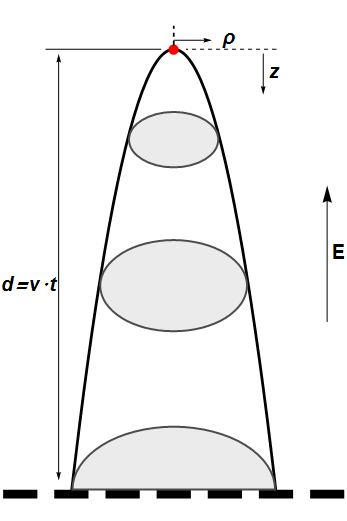
Figure 1: Illustration of the diffusion process starting from a point source to the detection plane indicated by dashed line. The diffusion in the longitudinal direction (along the drift direction) is generally expected to be smaller than that of the transverse direction. The standard deviation of the electron swarm (indicated by the shaded ellipses in the figure at three drift times) is expected to follow Eq. (9).

As the field approaches zero, the electrons gain so little energy from the field between the elastic atomic collisions that they come to thermal equilibrium with the medium. In this case, the diffusion coefficients are given by the Einstein-Smoluchowski relation [18, 19]:

$$D=\frac{kT}{e}\mu,$$ (10)

where $kT=0.0075$ eV for argon at the normal boiling point (87.3 K), $e$ is the electron charge, and $\mu$ is the electron mobility (the electron drift velocity $v$ per unit electric field $E$). At low fields, when the electrons are in equilibrium with the medium, the mobility and the electron temperature become constants. As the field is increased and the electrons are no longer in thermal equilibrium with the medium, the Einstein-Smoluchowski relation is taken to define the electron temperature. The electrons acquire energy from the field so that their temperature exceeds the thermal limit. The mobility decreases and the diffusion coefficients increase. This process has been quantified by generalized Einstein relations which obtain a quantitative relation between diffusion and mobility for electrons in strong electric fields using the energy dependence of the electron-atom collision cross section. The earliest version of this class of relations for electrons, as proposed by Wannier [20, 21], has the form:

$$D_{T} =\frac{kT}{e}\mu,$$ (11)

$$D_{L} =\frac{kT}{e}(\mu+E\frac{\partial\mu}{\partial E}),$$

where $kT$ is the electron temperature. The ratio of the longitudinal to the transverse diffusion coefficient is then expressed as:

$$\frac{D_{L}}{D_{T}}=1+\frac{E}{\mu}\frac{\partial\mu}{\partial E}.$$ (12)

At low electric fields, the mobility approaches a constant, and we have $D_{L}/D_{T}\approx 1$. As electric field increases, if the mobility decreases, then $D_{L}<D_{T}$, and vice versa.

3 Experimental Apparatus

Historically, there are three different techniques for the measurement of longitudinal diffusion: un-gridded [22, 23], gridded [24], and shuttered [25] drift cells. The electron source has typically been radioactive or a photocathode driven by a ultraviolet (UV) lamp. In this measurement, we chose to use a gridded drift cell because of its simplicity and similarity to the implementation of typical LArTPCs. For electron source generation, we employed an UV pulsed laser driving a semitransparent metal photocathode. The short pulse width and trigger stability of the laser allow timing information to be precisely synchronized.

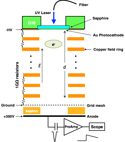
Figure 2: (color online) Illustration of setup for the electron drift velocity and diffusion measurement. See text for further discussion.

Fig. 2 shows a schematic view of the experimental apparatus. The photocathode is composed of a 22 nm thick Au film ($\sim$ 50% UV transmission) thermally evaporated onto a 1 mm thick, 10 mm diameter sapphire disk. The sapphire disk is mounted on a G10 dielectric ring at the top of the drift stack. The laser source is a frequency quadrupled, 4.66 eV, 60 picosecond pulse width Nd:YAG laser operating at 10 Hz repetition rate. The few $\mu$J of pulsed UV photons are focused onto a 1-meter long 600 $\mu$m diameter UV fused silica fiber with an numerical aperture (NA) of 0.22. The fiber is then coupled to a 600 $\mu$m diameter vacuum fiber feed-through followed by another 0.35-meter long 600 $\mu$m diameter in-vacuum UV fiber. The latter fiber ends directly on the back surface of the sapphire substrate. Photoelectrons are extracted into the LAr from the surface of the Au photocathode which is back-illuminated through this optical fiber delivery system with a maximum full beam size of $\sim$ 1 mm. The laser energy density at the photocathode is at least an order of magnitude lower than the measured $\sim$ 6 mJ/cm² threshold which leads to damages of gold films.

Negative high voltage is connected to a 200 $\mu$m thick phosphor bronze disk gasket that makes electrical contact to the photocathode. Ceramic screws are used to secure the gasket onto the G10 disk structure. Field shaping copper electrode rings with 2 mm thickness, 21.3 mm outside diameter, and a 15.7 mm open aperture are spaced 5 mm apart, on center, dictated by four G10 precision slotted rod structures. A series of 1 G$\Omega$ cryogenic compatible resistors make electrical contact to each ring and to the photocathode. A 300 $\mu$m thick Kapton ring is sandwiched between a +300 V biased anode disk below a grid mesh which is connected to the ground and to the last 1 G$\Omega$ resistor. The grid mesh has a wire width of 35 $\mu$m with 350 $\mu$m spacing and is mounted below a 250 $\mu$m thick phosphor bronze ring. The impact of thermal contraction on the distances at cryogenic temperature is negligible due to low thermal expansion coefficients of the materials. Given this setup, various drift distances from 5 mm to 60 mm can be arranged by adding or removing field shaping rings and moving the cathode assembly. The field between the grid mesh and the anode is called the anode collection field and kept at constant high value independent of the field in the drift region (drift field).

A thermocouple is placed near the photocathode to monitor the temperature. The drift stack is housed in a 0.5 liter cylindrical vacuum cell capable of being pressurized up to 1.66 bar limited by a pressure relief valve. As shown in Fig. 2, electron charge arriving at the anode plane is fed to a charge sensitive pre-amplifier (IO535) developed by Brookhaven National Laboratory which resides outside the cryogenic cell in ambient conditions. The pre-amplifier charge signal and its corresponding shaped and amplified pulses are recorded on an oscilloscope triggered by a fast photodiode that views a portion of the laser beam. The number of photoelectrons per pulse drifting through the stack to the anode ranges from $10^{3}$ to $10^{7}$ at bias fields increasing from 0.01 to $\sim$ 3 kV/cm. On the low end, this measurement is limited by amplifier noise which is $\sim$ 1350 rms electrons. With an additional 0.1 $\mu$s shaping amplifier, the noise charge can be further reduced to $\sim$ 230 rms electrons. In addition, the pre-amplifier responds to noise induced by the laser Q-switch particularly near the t = 0 trigger time. Therefore, in our procedure, 64 to 512 signal traces are averaged and subtracted from the corresponding signal trace acquired when the anode extraction field is off. This data acquisition process takes about one minute per measurement at a given drift field.

The entire system is baked to $\sim 90^{\circ}\rm C$ and pumped to $\sim 10^{-8}$ Torr prior to measurements. Great attention is taken to achieve the necessary high purity of argon gas and to avoid discharge at the high bias fields [26]. We start with high purity commercial (99.9999 vol %) Ar gas, which is then passed through a dry ice cold trap to reduce water vapor. The Ar gas is further purified by an Oxisorb filter to a ppb impurity level, and then transported through stainless steel pipes and valves. The argon in the cell is not further purified by recirculation. Finally, Ar is liquefied by external cooling with a mixture of liquid nitrogen and dry ice. A CCD camera is mounted on a top viewport to observe the LAr liquefaction process and also serves as a liquid level monitor. To measure the work function and the quantum efficiency of the photocathode, a fiber coupled continuous wave UV white light source (Energetiq LDLS) is wavelength selected by a monochromator, fiber-coupled to the in-vacuum fiber feedthrough of the LAr drift cell, and the photocurrrent leaving the photocathode is measured by a Keithley picoammeter connected to the photocathode.

4 Measurement and Raw Waveform Analysis

Electron drift velocity and longitudinal diffusion are determined with data taken at various drift distances and electric fields. This is crucial to fully categorize systematic uncertainties. Changing the drift distances requires breaking the vacuum and rearranging the drift stack. Fig. 3 shows the measurement parameter space in terms of the drift distance vs. electric field. At each drift distance, the maximum electric field that can be applied while avoiding high voltage breakdown is $\sim$ 3 kV. It is expected that this limit may be raised with an apparatus design that reduces sharp points causing field emission.

For each drift distance, the data taking procedure is

1. measurement of electron charge versus drift field at 10^-8 Torr vacuum at room temperature,

2. injection of ultrahigh purity Ar gas at up to 1.5 bar pressure into the test cell, following by charge measurement in gas Ar at room temperature,

3. conductive cooling of the drift cell to the LAr temperature while passively maintaining the temperature at 87 $\pm$ 1 K and pressure of the drift cell to $1.2\pm 0.1$ bar of gas Ar,

4. charge measurements at various drift fields in LAr.

The cooling process in step 3 generally takes $\sim$ 1 hour; the measurements in step 4 typically take several hours. It is important to note that LAr drift data are taken only when the thermocouple reading is 87 $\pm$ 1 K and the CCD camera indicates no obvious turbulence in the liquid argon.

The pressure measurements imply a temperature ranging from 88.2 K to 89.8 K at the surface of the LAr, in coexistence with the gas. This is distinctly higher than the temperature of 87 $\pm$ 1 K measured at the cathode. We attribute this difference to a presumed temperature gradient established in the LAr by cooling the Ar container from the bottom with the top near room temperature. Since no solid formation was observed during the measurements, we assume a minimum temperature of 84 K at the bottom of the cell. For these reasons we assign a mean temperature for the measurements in LAr of 87${}^{+1}_{-3}$ K. The effect of the temperature and pressure uncertainties is discussed in Sec. 6.2 and Sec. 6.3.

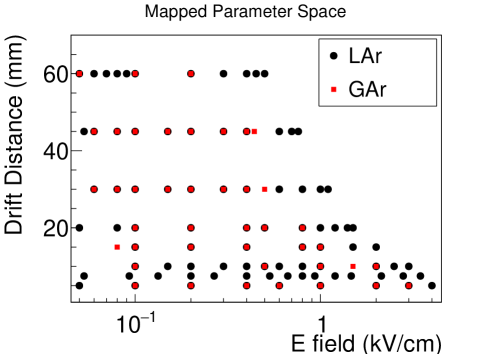
Figure 3: (color online) Summary of all data taken in liquid argon (LAr) and gas argon (GAr) in terms of the drift distance and the electric field. Data above 0.1 kV/cm was used for diffusion measurements. The boundary at high fields for each drift distance is limited by high voltage breakdown.

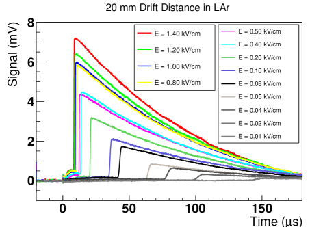
Figure 4: (color online) Representative raw signals in LAr at 20 mm drift distance are shown for various electric fields. The rising edges of the signals migrate toward the time zero with the increase of the electric field.

Fig. 4 shows a representative set of pre-amplifier output data taken in LAr at 20 mm drift distance. Time zero is defined by the laser pulse trigger. The rapid rise of the signal corresponds to the time when the electron swarm generated at photocathode has passed through the grid mesh. The position and width of the rise correspond to the drift time and diffusion time, respectively. The slow exponential signal decay is due to the discharge by the feedback resistor on the pre-amplifier. The slow rise prior to the onset of the main signal is due to some non-negligible residual charge leaving the anode or arriving at the cathode and does not alter the drift electron signal shape. The reduction of signal height as the electric field is decreased due to the decrease in quantum efficiency at low electric field and to the finite electron lifetime in LAr. The effect of the electron space charge is negligible because of the low charge density produced at the photocathode (see Ref. [13]), which will be further discussed in Sec. 6.3.

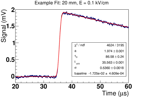
Figure 5: An example fit of Eq. (13) is shown. The uncertainty of each data point represents the size of estimated electronic noise and is treated to be uncorrelated in the fit. The uncertainty of the data are enlarged to make the reduced chi-square $\chi^{2}/NDF$ to unity, which leads to increased uncertainties of fitted parameters.

The raw signal is fitted with a functional form of

$$f(t,\sigma,\tau_{D},a)=a\cdot e^{\frac{\sigma^{2}-2t\cdot\tau_{D}}{2\tau_{D}^{2}}}\cdot\left(1+{\rm Erf}\left(\frac{-\sigma^{2}+t\cdot\tau_{D}}{\sqrt{2}\tau_{D}\cdot\sigma}\right)\right),$$ (13)

which is a convolution of a Gaussian function approximating the electron swarm and a step response function with damping representing the response of the pre-amplifier. Here, $a$ is the normalization factor that is proportional to the number of electrons in the swarm, $\sigma$ is the standard deviation of the Gaussian function which describes the longitudinal diffusion, $\tau_{D}$ is the decay constant of damping, and $t$ is the drift time. To accommodate the slow rise before the main signal, an additional parameter for the baseline shift is added. A typical fit is shown in Fig. 5. The uncertainty of each data point is the size of electronic noise, which is estimated by the standard deviation of the baseline. This type of uncertainty is treated as uncorrelated during the fit, and statistical uncertainties of the fitted parameters are adjusted accordingly to make the reduced chi-square $\chi^{2}/NDF$ unity. Systematic uncertainty due to the finite fitting range is estimated by changing the fitting range by 20%.

5 Systematic Uncertainties

The systematic errors in measuring drift velocities and diffusion coefficients caused by neglecting the higher order terms in the expansions of Eq. (2) are negligible for our measurements. We have measured the electron lifetime in our apparatus, and found that it ranges from 66 $\mu s$ ($\lambda$ = 0.3 cm^-1) to 530 $\mu s$ ($\lambda$ = 0.009 cm^-1). For these conditions, the expansion variables $D_{L}/(dv)$ and $D_{L}\lambda/v$ are at their maximum values at lowest fields and shortest drift distances. For 5 mm drift distance and 0.1 kV/cm field, they have values of 2.2 $\times 10^{-4}$ and 3.4 $\times 10^{-5}$ respectively. The largest bias in neglecting all but the first term in the expansion of Eq. (2) for this field and drift distance are 0.03% for drift velocity and 0.3% for diffusion time. For fields at which the electrons are in thermal equilibrium with the LAr ( $<\sim$ 0.1 kV/cm), the value of $\alpha$ can be computed using the Einstein-Smoluchowski relation to be $\alpha=\epsilon_{L}/\Delta V$, where $\Delta V$ is the potential drop over the drift distance and $\epsilon_{L}$ is the electron energy in volts. For higher fields and longer drift distances the errors are smaller.

The second systematic uncertainty is from the impulse response function of the pre-amplifier. The integration time of the pre-amplifier is $\tau_{I}$. In this case, the full form of signal response function is

$$f(t,\sigma,\tau_{D},a,\tau_{I})=a\cdot e^{\frac{\sigma^{2}-2t\cdot\tau_{D}}{2\tau_{D}^{2}}}\left(1+{\rm Erf}\left(\frac{-\sigma^{2}+t\cdot\tau_{D}}{\sqrt{2}\tau_{D}\cdot\sigma}\right)\right)$$ (14)

$$+a\cdot e^{\frac{\sigma^{2}-2t\cdot\tau_{I}}{2\tau_{I}^{2}}}\left(-2+{\rm Erfc}\left(\frac{-\sigma^{2}+t\cdot\tau_{I}}{\sqrt{2}\tau_{I}\cdot\sigma}\right)\right),$$

where the first term has the same functional form as that in Eq. (13). Due to the smallness of the $\tau_{I}$, the above equation is difficult to evaluate numerically without a computational demanding integration. Since the full functional form is not suitable in the large-scale fitting of the data, Eq. (13) is used instead to extract the drift and diffusion time. In this case, $\tau_{I}$ contributes to both the extracted drift and diffusion time (i.e. the rise time) of the electron signal by adding additional time, which needs to be corrected. This effect was directly calibrated by fitting the electron signal measured in vacuum. The contribution to the drift time and diffusion time due to $\tau_{I}$ is determined to be 31 $\pm$ 2 ns and 33 $\pm$ 5 ns, respectively. The systematic uncertainty due to different fitting functions (Eq. (13) vs. Eq. (14)) is negligible.

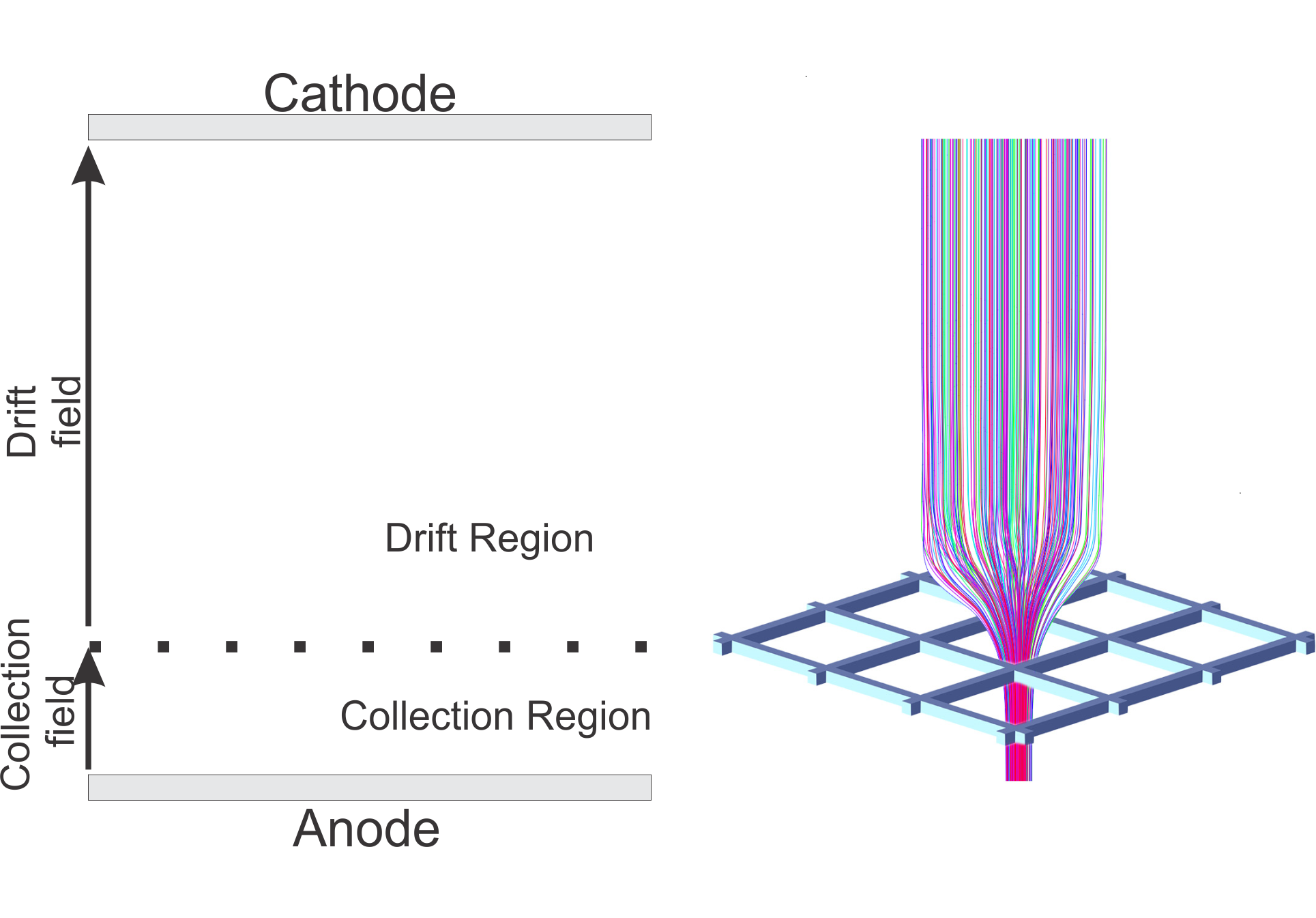
Figure 6: (Left) The scheme of the electron signal simulation. The electric field is computed with the MAXWELL 3D in the entire geometry (i.e. including both the drift and collection regions) with proper boundary conditions. (Right) The simulated electron trajectories are plotted with different colors respect to the grid mesh. The width of a grid cell is 350 $\mu$m. The curved trajectories lead to a bias on the extraction of both drift time and diffusion time which are corrected in the analysis. See text for further discussions.

The largest systematic uncertainty is caused by the electron drifting from the grid mesh to the anode. The grid mesh is installed at 300 $\mu$m from the anode. The purpose of the grid mesh is to screen the anode from the slow signal induced by the electrons in the drift region. The voltage at the anode is maintained at 300 V and the grid is at ground, creating a 10 kV/cm electric field in the collection region, which is much higher than applied electric field in the drift region (0.01 - 3 kV/cm). A perfect grid would separate the drift and collection regions with a constant field on both sides. In reality, electric field “leaks” through the grid from the high-field region (i.e. the collection region) to the low-field region (i.e. the drift region). This effect leads to a bias in estimating the drift field. In order to evaluate this effect, the electric field in the drift cell is computed by MAXWELL 3D [27] using a geometric model of the apparatus. The scheme and resulting electron trajectories of the simulation are shown in Fig. 6. Fig. 7 shows the computed electric field for a set of points along the diagonal axis of the cell. The electric field is largely non-uniform within -200 to +400 $\mu$m distance from the grid mesh.

Another possible systematic uncertainty is the imperfect uniformity of the electric field in our drift stack. We used MAXWELL 3D to compute the electric fields for the full geometry including the drift stack, cryostat walls, and cables etc. Ray tracing calculations in these fields show a very small focusing of the electron swarm as it drifts to the grid. This causes the transverse width of the beam distribution to decrease by about 0.08 mm, which is significant compared to the estimated transverse diffusion especially for short drift distances. However, the variation in the drift time caused by the variation in the path lengths is much smaller fractionally, systematically increasing the longitudinal diffusion time by a maximum of 0.31 ns compared to the measured diffusion time of 42 ns for the highest fields reported. This is a maximum systematic increase of 0.7% in the longitudinal diffusion coefficient. This systematic, one sided error in the diffusion is typical of the calculations for all the drift lengths. Any other instrumental effects producing time invariant fields also can only increase the apparent measurement of diffusion. Among such effects that have not been modeled are: focusing through the grid mesh; non-co-planarity of the grid, anode, cathode and field rings; imperfect spacing and shape of the gradient rings; charging of support insulators; and imperfect matching of the gradient resistor values. Including the effects of these imperfections on the central field in the drift cell increases the assigned error for field imperfections to ${}^{+2}_{-0}$%. This one-sided systematic error is still small compared to the statistical error in the analysis.

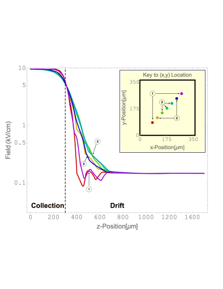
Figure 7: (color online) MAXWELL 3D computed electric field close to the grid mesh are shown for a set of points along the diagonal axis of a grid cell. For the expected electric field in the collection and drift region of 10 and 0.1 kV/cm, the achieved fields are respectively lower and higher than the expected fields due to the field leakage through the grid. These curves are labeled with numeric indexes by group on the diagonal line.

The electron signals are simulated with a ray tracing technique that begins with randomly distributed electrons within the dimension of a single grid cell (350 $\mu$m wide on each dimension). As shown in the right panel of Fig. 6, 200 electrons with zero initial velocity are generated 5 mm above the grid plane. The electron trajectories are solved using the computed electric field and expected electron mobility from a global fit of the existing world data. The electron trajectories are focused into the center of the grid cell when electrons are close to the grid mesh, as shown in Fig. 6. Therefore, three sources of systematic uncertainties arise due to the imperfect grid plane:

• The drift distance is measured to the grid mesh. The electrons take some additional time to drift far enough toward the anode to cause the signal rise of 50% (the stop for the drift time measurement clock). In addition, the trajectories starting far from the center of the cell are longer than the central trajectory due to the focusing as shown in the right panel of Fig. 6. This variation also increases the drift time. This is negligible for all but the shortest drift distances and highest drift fields as will be discussed in Section 6.2. The tightly focused bundle of trajectories for low drift fields lead to a spreading of the drift times over the grid cell, which increases the signal rise time over that due to longitudinal diffusion only. This effect is expected to be largely independent of the drift field. The ray tracing simulation suggests that the magnitude of longitudinal diffusion is comparable to the electron drift time from the grid plane to the anode plane. Therefore, we use the expected drift time from grid to the anode plane to estimate the contribution of non-uniform electron trajectory to the diffusion time and assign a conservative 100% uncertainty in the analysis. This effect is negligible for GAr, but important for the LAr measurement.

• When the drift field is small, the leakage field leads to a significant bias on the magnitude of the field in the drift region. As shown in Sec. 4, we limit our diffusion measurement to fields above 0.1 kV/cm. We further estimate the uncertainty due to this effect with an empirical formula (see Section 6.3).

Additional systematic uncertainties include the measurement of drift distance (measured to 0.1 mm) and the control of experimental conditions (pressure and temperature). For LAr the temperature is accurate to 1 K. For GAr, it is controlled to the room temperature, and the pressure is controlled to 2 mbar. The resulting uncertainties will be discussed in Sec. 6.2 and Sec. 6.3 for electron mobility and diffusion measurements, respectively.

6 Results

6.1 Quantum Efficiency of Au Photocathode

Several batches of Au films are measured and consistently have a work function of 4.17 eV, 4.10 eV, and 3.89 eV in vacuum, in GAr, and in LAr, respectively, see Fig. 8. The 0.28 eV lowering of work function in LAr indicates a negative electron affinity, which is similar to previous measurements with Zn [28] and Ba [29] photocathodes. Although the drift photoelectrons bear this excess kinetic energy on ejection from the cathode, they come to thermal equilibrium through collisions with argon atoms in a time less than 1 ns, and a distance less than a few microns [30]. Therefore the negative electron affinity has no impact on drift and diffusion measurement.

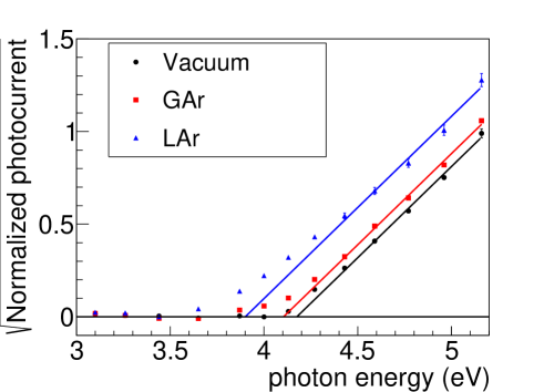
Figure 8: (color online) The square-root of photocurrents normalized to the value at 5.16 eV from photocathode are shown with respect to the photon energy. Straight line fits on the data between 4.43 and 5.14 eV are performed to extract the work function at y=0 intercept. Representative error bars are shown in the fitted region.

The quantum efficiency (QE) is defined as the number of electrons leaving the photocathode per number of UV photons irradiating the back surface of the photocathode. QEs of $\sim 10^{-5}$, $\sim 2\times 10^{-6}$, and $\sim 10^{-7}$ are obtained when the photocathode is operated in vacuum at room temperature, 1500 $\pm$ 2 mbar of high purity Ar gas at room temperature, and at LAr temperature, respectively. Despite the QE drop of nearly 2 orders of magnitude in LAr, the photocathode provides $10^{5}$ electrons with $\sim 1\mu$J of UV photons which are sufficient for the measurements described here.

The factor of $\sim 5$ drop in the QE from vacuum to 1500 mbar of Ar gas is due to the increase of the potential barrier caused by the Ar atoms adsorbed on the photocathode, which can be recovered by pump down of the system and proper baking. The factor of $\sim 50$ drop in the QE from vacuum to LAr is mainly caused by electron back diffusion to the photocathode. Although the negative electron affinity of -0.28 eV reduces the work function of the photocathode, the field of the image charge and the low drift velocity of electrons in LAr favor strong back diffusion so that most photoelectrons return to the photocathode. A random walk simulation of the diffusion process for an electron leaving the cathode with excess energy is presented in [31]. The results of this simulation suggest that when an electron starts on the gold-LAr interface with an electron energy $\sim$ 0.5 eV and propagates in a field $<$ 1 kV/cm, the survival rate of the photoelectrons is $\sim 3$ %. This result is consistent with the QE measurements, and also qualitatively agrees with other measurements on metal photocathodes operated in LAr [28].

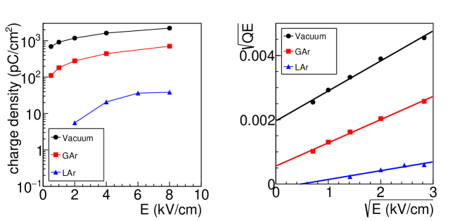
Figure 9: (color online) (Left panel) Charge density from the photocathode is plotted versus the electric field for vacuum, GAr and LAr. (Right panel) The square-root of the quantum efficiency is plotted against the square-root of the electric field. Linear fits of the data are shown as well.

Photoemission is a statistical process which can be described, to the first approximation, by the well-known three-step Spicer photoemission model [32]: (i) absorption of light to excite the electrons from an initial state to a final state, (ii) transport of excited electrons to the surface, and (iii) escape of the electrons by overcoming a potential barrier. The QE is thus given by the Fowler law:

$$\text{QE}=k(h\nu-\phi_{0}+\alpha\sqrt{\beta\cdot E})^{2},$$ (15)

where $k$ is a constant that depends on the material, $\phi_{0}$ is the work function of the metal, $\alpha=\sqrt{e/4\pi\epsilon_{0}}$, $e$ is the electron charge, $\epsilon_{0}$ is the vacuum dielectric constant, $E$ is the extraction electric field, $h\nu$ is the photon energy, and $\beta$ is the field enhancement factor. The left panel of Fig. 9 plots the charge density leaving the photocathode versus the bias field, while the right panel of Fig. 9 plots $\sqrt{\text{QE}}$ against the $\sqrt{E}$. The measured QE exhibits a linear dependence as predicted by Fowler’s law in vacuum and in low pressure of gaseous argon but has some deviations in liquid argon. A more quantitative evaluation of these deviations requires measurements outside the current scope.

6.2 Drift Velocity in GAr and LAr

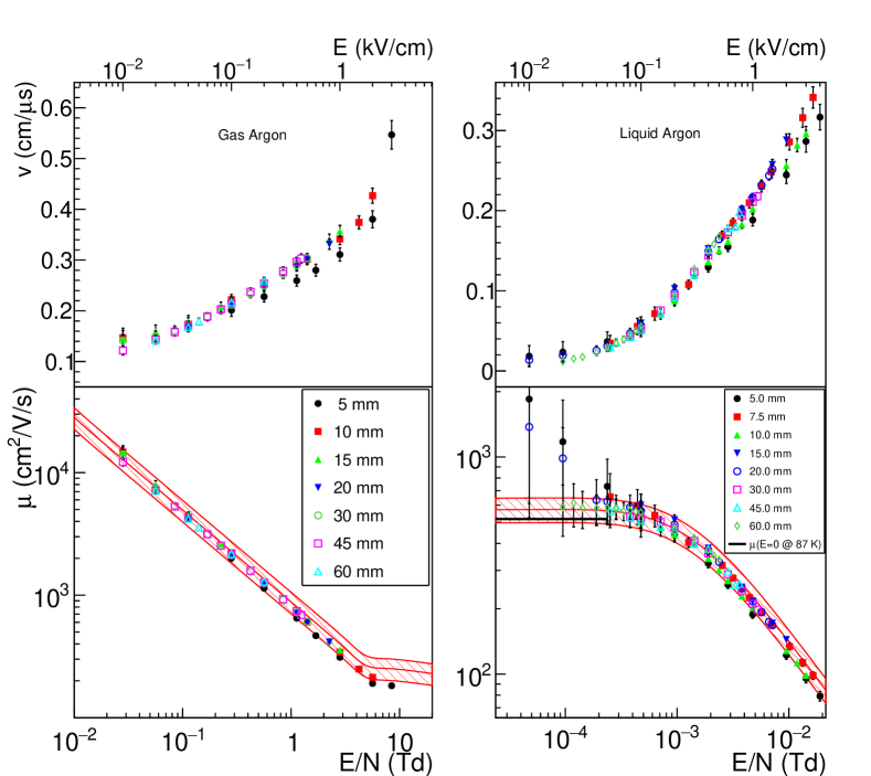
Figure 10: (color online) Electron drift velocity (top panels) and electron mobility (bottom panels) are shown with respect to the electric field for various drift distance settings for GAr (left panels) and LAr (right panels). The nominal electric field $E$ (top x-axis) and the reduced field $E/N$ (bottom x-axis) which is the $E$ normalized with the number density of argon with the unit of $Td\equiv 10^{-17}$ V$\cdot$ cm² are both presented for direct comparison. The red bands in the mobility plots (bottom panels) represent the global fit and their uncertainties. For LAr, the expected mobility at zero electric field ($\sim$ 518 cm²/V/s) is plotted. See text for further discussions.

The drift velocity and mobility are defined as

$$v=\frac{d}{t}=\mu\cdot E.$$ (16)

Here, $d$ is the drift distance, $t$ is the drift time, $\mu$ is the mobility, and $E$ is the electric field. The drift distance $d$ is measured to an uncertainty of 0.1 mm by the position of the anode and cathode on the drift stack. The drift time $t$ is calculated from the measured drift time by correcting for the time shift due to the response of the pre-amplifier and for the time which electrons take to drift from the grid mesh to the anode plane. The pre-amplifier time offset is measured to be $31\pm 2$ ns with respect to the laser trigger from the calibration data taken in vacuum. The drift time between the grid plane and the anode plane for GAr is calculated to be $15\pm 5$ ns based on drift velocity data from Refs. [33, 34, 35, 36, 37, 38, 39, 40, 41, 42, 43, 44]. For LAr, this correction is calculated to $65\pm 7$ ns based on data from Refs. [45, 46, 47, 48, 29, 49, 50, 51, 52, 53, 54, 55, 56, 57, 58]. The additional drift time due to grid-to-anode drift and curved trajectories is estimated with ray tracing simulation to be $15\pm 15$ and $65\pm 65$ ns for GAr and LAr, respectively. These corrections are small compared to the measured drift time ranging from a few $\mu$s to a few hundred $\mu$s. The uncertainties due to temperature and pressure variations are estimated to be 3% and 5% assuming the general $T^{-3/2}$ temperature dependence of the mobility [59]. For LAr, this uncertainty is confirmed by repeated sets of data taken over a period of several hours at 20 mm drift distance and 0.5 kV/cm electric field.

Beside these uncertainties, an additional systematic uncertainty is added due to the leakage field as discussed in Sec. 5. The leakage field leads to a sizable difference in LAr electron mobility measured from different drift distances for electric field below 0.1 kV/cm. Due to the difficulty in precisely predicting the size of leakage field in all the configurations, no correction was made to our results. Instead, conservative uncertainties for GAr and LAr were estimated by quoting a 100% change in results when including empirical leakage field assumed to be uniform in the entire drift region:

$$0.025\cdot\sqrt{\frac{5mm}{d}}$$ (17)

in kV/cm. The format of the leakage field was then deduced, so that the zero-field electron mobility in LAr then satisfied the expected results of $\sim$518 cm²/V/s. The impact of this effect is much smaller for GAr due to much weaker electric field dependence in our region of interest for the drift velocity. For the diffusion measurement, we limit the data to a region with expected electric field larger than 0.1 kV/cm, where the leakage field effect has a smaller effect.

Fig. 10 shows electron drift velocity (top panels) and electron mobility (bottom panels) as a function of the drift field for various drift distances for GAr (left panels) and LAr (right panels). The nominal electric field $E$ and reduced field $E/N$ which is the $E$ normalized with the number density of argon with the unit of $Td\equiv 10^{-17}$ V$\cdot$ cm² are both presented for direct comparison. This normalization is in particular importance for GAr comparison due to its wide range of density variation at different pressures and temperatures. The red curve and band in the bottom panels are the global fit of world data, in LAr data from Ref. [45, 46, 47, 48, 29, 49, 50, 51, 52, 53, 54, 55, 56, 57, 58], GAr data from Ref. [33, 34, 35, 36, 37, 38, 39, 40, 41, 42, 43, 44].

The relative uncertainties for the global fit are about 13% and 20% for LAr and GAr, respectively. For GAr the extracted electron velocities are largely consistent among different drift distances except for the 5 mm drift, which indicates additional experimental uncertainties unaccounted for in the analysis in this setting. As shown in the Sec. 2, the drift time is a parameter used in the extraction of diffusion coefficient. A 7% additional uncertainty was added to the measured drift time in order to take into account this discrepancy.

For LAr, the extracted electron velocities at various drift distances are consistent with each other. The measured velocities for 5 mm and 10 mm show a small discrepancy at high electric field, which again indicates additional experimental uncertainties unaccounted for in the analysis. A 5% additional uncertainty was added to the measured drift time in order to extract the diffusion coefficient conservatively. The comparison of the extracted LAr electron mobility data are in excellent agreement with the global fit for electric fields larger than 0.1 kV/cm. At electric fields smaller than 0.1 kV/cm, the leakage field effect leads to significant systematic uncertainties. The black line represents the expected electron mobility $\sim$ 518 cm²/V/s at 87 K, which is used as a guideline to estimate the strength of leakage field. For the diffusion result discussed in the next section, we are restricted to drift fields larger than 0.1 kV/cm.

6.3 Longitudinal Diffusion in GAr and LAr

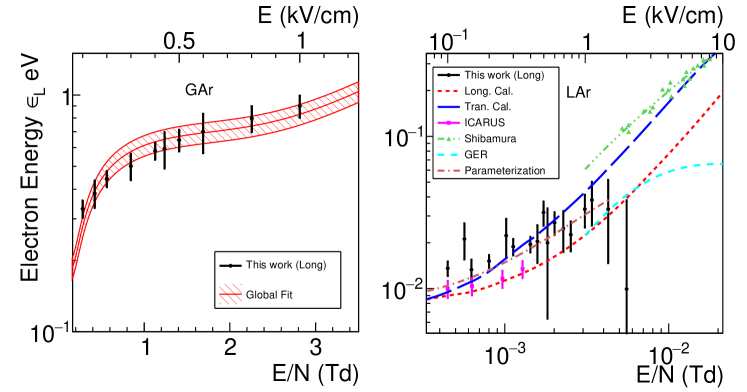
Figure 11: (color online) The extracted electron energy $\epsilon_{L}$ for the longitudinal diffusion is plotted versus the electric field for GAr and LAr. The nominal electric field $E$ (top x-axis) and reduced field $E/N$ (bottom x-axis) which is the $E$ normalized with the number density of argon with the unit of $Td\equiv 10^{-17}$ V$\cdot$ cm² are both presented for a direct comparison. The red band in the GAr panel represents the global fit and its uncertainty. For LAr, our data are systematically higher than the prediction of Atrazhev-Timoshkin [2]. The red line represents the longitudinal electron energy and blue line represents the transverse electron energy. The magenta points are deduced from the measurements by ICARUS [1] at low electric field (see text for details). The green dots represent the transverse electron energy data reported by Shibamura [13] at high electric fields. The dashed cyan curve is the calculated longitudinal electron energy using the general Einstein relation (Eq. (11) and Eq. (12)) from the interpolation (dashed green line) to the transverse electron energy reported by Shibamura [13]. The brown dot-dashed line represents the parameterization we introduced. Details are presented in the appendix.

The longitudinal diffusion time defined in Eq. (9) can be equivalently expressed as:

$$\sigma_{L}=\sqrt{\frac{2\epsilon_{L}\cdot d}{E}}\cdot\frac{t}{d}.$$ (18)

Here, $\epsilon_{L}=eD_{L}/\mu$ is the effective energy of electron, $D_{L}$ is the longitudinal diffusion coefficient, $\mu$ is the electron mobility, $e$ is the electron charge, $d$ is the drift distance, $E$ is the electric field, and $t$ is the drift time. In our experimental setup, we expect additional contributions from systematic errors due to the measured drift time. The contribution from the response of the pre-amplifier is determined with the calibration data in vacuum to be $33\pm 5$ ns. As discussed in Sec. 5, the contribution due to grid-to-anode drift and curved electron trajectories are estimated to be $15\pm 15$ and $65\pm 65$ ns for GAr and LAr, respectively. In this case, Eq. (18) is modified as:

$$\sigma^{2}_{L}=\epsilon_{L}(E)\cdot\frac{2t^{2}}{d\cdot E}+c^{2}(d),$$ (19)

with $c(d)$ being the constant term that depends on the drift distance. The longitudinal diffusion time $\sigma_{L}$ and drift time $t$ depends on both the electric field $E$ and the drift distance $d$. Therefore, the effective electron temperature $\epsilon_{L}(E)$, as a function of the electric field $E$ can be extracted through a simultaneous fit of all the results of longitudinal diffusion and drift time by minimizing the following $\chi^{2}$ function:

$$\chi^{2}=\sum_{i}\frac{\left(\sigma^{2}_{L}-\epsilon_{L}(E_{k})\cdot\frac{2t^{2}}{d_{j}\cdot E_{k}}-c^{2}(d_{j})\right)^{2}}{4\sigma_{L}^{2}(\delta\sigma_{L})^{2}+\frac{4t^{4}\cdot\epsilon_{L}^{2}(E_{k})}{d_{j}^{2}E_{k}^{2}}\cdot\left(\frac{(\delta d_{j})^{2}}{d_{j}^{2}}+\frac{(\delta E_{k})^{2}}{E_{k}^{2}}+\frac{4(\delta t)^{2}}{t^{2}}\right)}+\sum_{j}\frac{\left(c(d_{j})-c_{0}\right)^{2}}{(\delta c)^{2}},$$ (20)

where the notation $\delta X$ represents the uncertainty of the physical quantity $X$. The notation $i$ represents the $i$th data point with electric field $E_{k}$ and drift distance $d_{j}$. The constant term at each drift distance is constrained around the expected value with its uncertainty. Beside the uncertainties of measured drift time as discussed previously, the uncertainty of the electric field is estimated with the empirical formula in Eq. (17). Additional uncertainties of 1% and 3% are included for GAr and LAr, respectively, to take into account the variations in experimental conditions in terms of temperature and pressure. This estimation was obtained assuming a linear temperature dependence for the electron energy. Furthermore, due to the leakage field effect, the fit was limited to data taken higher than 0.1 kV/cm drift field where the leakage field effect is properly estimated as suggested by the mobility data discussed in Sec. 6.2.

The extracted electron energy $\epsilon_{L}$ for GAr and LAr are shown in Fig. 11. For GAr, the reduced chisquare $\chi^{2}/NDF=3.3/23$ indicating conservative systematic uncertainties. The extracted electron temperatures are consistent with a global fit to the world data [37, 41, 42, 43, 44]. The consistency between our data and the global fit again confirms the validity of the analysis procedure.

For LAr, the reduced chisquare $\chi^{2}/NDF=114.6/43$ indicating additional unknown systematic uncertainties. In order to minimize the bias to the results due to these uncertainties, an additional 8% uncorrelated uncertainty is added to each of the measured diffusion times. The new fit shown, in the right panel of Fig. 11, gives a reduced chisquare $\chi^{2}/NDF=45.8/43$. The ICARUS group reports measurements for the square of the diffusion time vs. drift time at 92 K and four fields from 100 to 350 V/cm in Fig 15. of Ref.  [1]. We have fit this data to obtain longitudinal diffusion coefficients at the four fields. They also report drift velocity measurements at 92 K for fields above 200 V/cm. In order to convert the diffusion constants to effective electron temperatures using the Einstein-Smoluchowski relation (Eq. (10)), we have obtained the corresponding mobilities by fitting their data for mobility at 92 K (contained in Fig. 13 of Ref. [1]) to the functional form we used for the global fit (Eq. (21) in the Appendix). These effective energies at 92 K are scaled to 87 K assuming a linear $T$ dependence of the effective electron energy. This is certainly correct at low fields, where the electrons are in thermal equilibrium with the LAr, and is probably quite accurate for the entire range of the ICARUS data set, for which the mobility is still close to the zero field value. Our results are higher than the converted results from ICARUS.

At high electric fields, there is no existing data on the longitudinal diffusion. On the other hand, transverse diffusion results exist for electric field $>$ 1.7 kV/cm from Shibamura [13]. As discussed in Sec. 2, the longitudinal electron energy can be related to the transverse electron energy through the general Einstein relation. Using Eq. (11) and Eq. (12) together with the electron mobility from the global fit (Fig. 10), the transverse electron energy results from Ref. [13] (green points in Fig. 11 and green dashed line for interpolation) are converted into longitudinal electron energy (dashed cyan curve in Fig. 11). The deduced longitudinal electron energies are consistent with our data at high electric fields.

The formula of our fit to a large selection of the world’s data for electron mobility in LAr is presented in the Appendix. A similar parameterization is applied to the existing data on longitudinal electron energy as shown in Fig. 11 whose formula is also presented in the Appendix.

Our results are also compared to a calculation of the transport properties of LAr by Atrazhev-Timoshkin [2], which gives the transverse and longitudinal electron energy as a function of field near the triple point (their Fig. 4). These calculations are shown in Fig. 11. Our data are systematically higher than this calculation. At zero electric field, the electron temperature is expected to be the same as that of the LAr. The fact that both ICARUS’ and our data are higher than this value (0.0075 eV at 87 K) at low electric field is puzzling. In the ICARUS paper [1], an additional correction to $D_{L}$ (and thus to the electron energy) caused by the space charge effect (Coulomb repulsion of the electron cloud) was quoted. This correction was estimated by using an approximate model described in Ref. [13]. The resulting electron energy from ICARUS after applying the correction is much lower than the LAr temperature. We performed the same calculation and found that the correction for our conditions is small due to the lower electron density in our measurements for both drift and collection region. The focusing of the electron trajectories through the grid mesh causes a negligible increase in any space charge broadening since the transit time through the grid mesh is a negligible fraction of the total drift time and the total charge is divided among many grids. We also note that Ref. [13] declined to apply space charge effect they computed to their measurements. We agree with Ref. [13] and do not include the space charge effect correction in our results. Nevertheless, we should comment that the space charge effect at low field with short drift distance and maximum space charge density could be more significant and may possibly explain the discrepancy between our effective energy to the theoretical calculation. This can best investigated by measurement with different space charge density, which can be achieved by changing the transverse source dimensions.

7 Summary

LArTPCs is a key detector technology for neutrino physics in searching for new CP violation and determining the mass hierarchy. Understanding the performance of LArTPCs requires a good knowledge of electron transport in LAr. In particular, diffusion of electrons in LArTPCs limits the spatial resolution of tracks with long drift distances. At 500 V/cm electric field, the longitudinal diffusion coefficient is $D_{L}=7.2$ cm²/s from measurements, and the transverse diffusion coefficient is $D_{T}=$ 12.0 cm²/s by extrapolating existing data measured at high field [13]. For a 3.6 meter drift, as proposed in the DUNE far detector, the diffusion limited resolution will be around 1.8 mm (1.1 $\mu$s in time) longitudinal and 2.5 mm transverse to the electric field at 500 V/cm for a track produced near the cathode. This implies spatial resolution for the longest drift distance will not be improved with signal sampling time shorter than 1 $\mu$s and wire pitch much less than 3 mm. For extremely long drift distances, such as the 20 meter drift distance proposed for the GLACIER detector, the diffusion limited resolution will be 4.2 mm (2.7 $\mu$s in time) longitudinal and 7.7 mm transverse to the electric field of 500 V/cm. These values become important for distinguishing very short tracks from point like depositions which must drift for long distances. An important example include distinguishing supernova neutrinos from the more nearly point-like tracks made by the $\alpha$ and $\beta$ particles from the decay of radioactive contaminants in the LAr (such as ³⁹Ar). Since diffusion plays a non-negligible role in determining signal shape in large LArTPCs, a good knowledge of diffusion is important in simulating the device responses and in extracting track coordinates.

In this paper, we present our measurement of the electron mobility and longitudinal diffusion coefficients in GAr and LAr. Our experimental setup uses a thin gold photocathode as a bright electron source. The work function and quantum efficiency of the gold photocathode are measured in vacuum, GAr, and LAr. Our result shows that the gold photocathode is a good candidate as a calibration source for future large LArTPCs.

The measured electron mobility in GAr and LAr and longitudinal electron diffusion coefficient (expressed as the electron energy) in GAr, over a wide range of electric fields, show good agreement with fits of existing world data. This validates our experimental approach to systematically measure the longitudinal electron diffusion coefficients in LAr for electric fields between 100 and 2000 V/cm. The extracted longitudinal electron energy in LAr in the region between 100 and 350 V/cm shows a discrepancy with previous ICARUS measurement. In the region of 350 to 2000 V/cm, our results represent the world’s best measurement. Over the entire electric field range, the measured longitudinal electron energy is found to be systematically higher than the prediction of Atrazhev-Timoshkin [2].

Our results are limited by the systematic uncertainties coming from i) leakage field effects due to imperfection of grid mesh and ii) unaccounted systematic uncertainties in the diffusion time likely due to the control of experimental condition and noise. A new experimental setup with improved design of the grid mesh and better control of experimental conditions has been constructed. Improved measurements on the electron temperature are expected and will be reported.

It is also desired to extend the measurement to transverse diffusion. While the longitudinal diffusion expresses itself as a spread in drift time, the transverse diffusion expresses itself as a spread in space. Therefore, the anode in the current apparatus is not sufficient to perform measurements of transverse diffusion. A new anode with fine position resolution is being designed for future transverse diffusion measurements.

8 Acknowledgments

This material is based upon work supported by the U.S. Department of Energy, Office of Science, Office of High Energy Physics and Early Career Research program under contract number DE-SC0012704.

Appendix

Global fit on electron mobility in LAr

The electron mobility data set used in our global data fit are from Ref. [45, 46, 47, 48, 29, 49, 50, 51, 52, 53, 54, 55, 56, 57, 58]. LAr temperature used in this global fit is 89 K. The data reported in the references are all scaled to this temperature with the temperature dependence of $T^{-3/2}$ [59]. The fitting function is a rational polynomial expressed as:

$$\mu=\frac{a_{0}+a_{1}E+a_{2}E^{3/2}+a_{3}E^{5/2}}{1+(a_{1}/a_{0})E+a_{4}E^{2}+a_{5}E^{3}}\left(\frac{T}{T_{0}}\right)^{-3/2},$$ (21)

where $E$ is the electric field in the unit of kV/cm and $a_{0}=551.6$ cm²/s is the electron mobility at zero field with temperature of $T_{0}$ = 89 K, $T$ is the LAr temperature. The fitting parameters are given in Table 1:

Table 1: Function paraemeters in Eq. (21)

$a_{0}$	=	551.6
$a_{1}$	=	7953.7
$a_{2}$	=	4440.43
$a_{3}$	=	4.29
$a_{4}$	=	43.63
$a_{5}$	=	0.2053

Parameterization on effective longitudinal electron energy

We also introduce a parameterization of the effective electron energy for the convenience of application. Both of our data and ICARUS’ data at low field are included. The parameterization is also in a form of rational polynomial

$$\epsilon_{L}=\frac{b_{0}+b_{1}E+b_{2}E^{2}}{1+(b_{1}/b_{0})E+b_{3}E^{2}}\left(\frac{T}{T_{1}}\right)$$ (22)

where $E$ is the electric field in the unit of kV/cm and $b_{0}=0.0075$ eV is the electron energy at $T_{1}$ = 87 K under zero field and $T$ is the LAr temperature. The parameterization can be applied to other temperatures with a linear temperature dependence of $T$.

Table 2: Function parameters in Eq. (22)

$b_{0}$	=	0.0075
$b_{1}$	=	742.9
$b_{2}$	=	3269.6
$b_{3}$	=	31678.2

The longitudinal diffusion coefficients $D_{L}$ in the range of 0.1 to 1.5 kV/cm can thus be expressed as defined by the Einstein relation in Eq. (10):

$$D_{L}=\frac{\mu\epsilon_{L}}{e}=\left(\frac{a_{0}+a_{1}E+a_{2}E^{3/2}+a_{3}E^{5/2}}{1+(a_{1}/a_{0})E+a_{4}E^{2}+a_{5}E^{3}}\right)\left(\frac{b_{0}+b_{1}E+b_{2}E^{2}}{1+(b_{1}/b_{0})E+b_{3}E^{2}}\right)\left(\frac{T}{T_{0}}\right)^{-3/2}\left(\frac{T}{T_{1}}\right),$$ (23)

with the parameters given in Tables. 1 and 2.

References

References

- [1] P. Cennini, S. Cittolin, J. Revol, C. Rubbia, W. Tian, et al., Performance of a 3-ton liquid argon time projection chamber, Nucl.Instrum.Meth. A345 (1994) 230–243. doi:10.1016/0168-9002(94)90996-2.
- [2] V. M. Atrazhev, I. V. Timoshkin, Trasport of electrons in atomic liquids in high electric fields, IEEE Trans. Dielectrics and Electrical Insulation 5 (1998) 450.
- [3] W. J. Willis, V. Radeka, Liquid argon ionization chambers as total absorption detector, Nuclear Instruments and Methods 120 (1974) 221.
- [4] C. Rubbia, The liquid argon time projection chamber: A new concept for neutrino detector, CERN-EP/77-08 (1977).
- [5] S. Amerio, et al., Design, construction and tests of the ICARUS T600 detector, Nucl.Instrum.Meth. A527 (2004) 329–410. doi:10.1016/j.nima.2004.02.044.
- [6] C. Anderson, et al., First Measurements of Inclusive Muon Neutrino Charged Current Differential Cross Sections on Argon, Phys.Rev.Lett. 108 (2012) 161802. arXiv:1111.0103, doi:10.1103/PhysRevLett.108.161802.
- [7] T. Alexander, et al., DarkSide search for dark matter, JINST 8 (2013) C11021. doi:10.1088/1748-0221/8/11/C11021.
- [8] A. Zani, The WArP Experiment: A Double-Phase Argon Detector for Dark Matter Searches, Adv.High Energy Phys. 2014 (2014) 205107. doi:10.1155/2014/205107.
- [9] B. Yu, D. S. Makowiecki, G. J. Mahler, V. Radeka, C. Thorn, B. Baller, H. Jostlein, B. T. Fleming, Designs of Large Liquid Argon TPCs — from MicroBooNE to LBNE LAr40, Phys. Procedia 37 (2012) 1279–1286. doi:10.1016/j.phpro.2012.03.737.
- [10] C. Adams, et al., The Long-Baseline Neutrino Experiment: Exploring Fundamental Symmetries of the UniversearXiv:1307.7335.
- [11] C. Adams, J. Alonso, A. Ankowski, J. Asaadi, J. Ashenfelter, et al., The Intermediate Neutrino ProgramarXiv:1503.06637.
- [12] M. Antonello, et al., A Proposal for a Three Detector Short-Baseline Neutrino Oscillation Program in the Fermilab Booster Neutrino BeamarXiv:1503.01520.
- [13] E. Shibamura, T. Takahashi, S. Kubota, T. Doke, Ratio of diffusion coefficient to mobility for electrons in liquid argon, Physical Review A 20 (6) (1979) 2547.
- [14] S. E. Derenzo, A. R. Kirschbaum, P. H. Eberhard, R. R. Ross, F. T. Solmitz, Test of a Liquid Argon Chamber with 20-Micrometer RMS Resolution, Nucl.Instrum.Meth. 122 (1974) 319. doi:10.1016/0029-554X(74)90495-9.
- [15] A. Fick, Ann. der. Physik 94 (1855) 59.
- [16] A. Fick, Phil. Mag. 10 (1855) 30.
- [17] P. Morse, H. Feshbach, Methods of Theoretical Physics, Part I, McGraw-Hill, New York, USA, 1953.
- [18] A. Einstein, Über die von der molekularkinetischen Theorie der Wärme geforderte Bewegung von in ruhenden Flüssigkeiten suspendierten Teilchen, Annalen der Physik 322 (1905) 549–560. doi:10.1002/andp.19053220806.
- [19] M. von Smoluchowski, Zur kinetischen Theorie der Brownschen Molekularbewegung und der Suspensionen, Annalen der Physik 326 (1906) 756–780. doi:10.1002/andp.19063261405.
- [20] G. H. Wannier, Motion of gaseous ions in strong electric fields, Bell System Technical Journal 32 (1) (1953) 170–254.
- [21] R. E. Robson, A thermodynamic treatment of anisotropic diffusion in an electric field, Australian Journal of Physics 25 (1972) 685.
- [22] S. R. Hunter, J. G. Carter, L. G. Christophorou, Electron transport measurements in methane using an improved pulsed townsend technique, Journal of applied physics 60 (1) (1986) 24–35.
- [23] H. Kusano, J. A. Matias-Lopes, M. Miyajima, E. Shibamura, N. Hasebe, Electron mobility and longitudinal diffusion coefficient in high-density gaseous xenon, Japanese Journal of Applied Physics 51 (11R) (2012) 116301.
- [24] D. K. Davies, L. E. Kline, W. E. Bies, Measurements of swarm parameters and derived electron collision cross sections in methane, Journal of Applied Physics 65 (9) (1989) 3311–3323.
- [25] J. Takatou, H. Sato, Y. Nakamura, Drift velocity and longitudinal diffusion coefficient of electrons in pure ethene, Journal of Physics D: Applied Physics 44 (31) (2011) 315201.
- [26] J. S. Townsend, V. A. Bailey, The motion of electrons in argon, The London, Edinburgh, and Dublin Philosophical Magazine and Journal of Science 43 (255) (1922) 593–600.
- [27] MAXWELL 3D (ANSOFT) http://www.ansys.com/Products/Simulation+Technology/Electronics/Electromechanical/ANSYS+Maxwell.
- [28] W. Tauchert, H. Jungblut, W. F. Schmidt, Photoelectric determination of v0 values and electron ranges in some cryogenic liquids, Canadian Journal of Chemistry 55 (11) (1977) 1860–1866.
-
[29]
B. Halpern, J. Lekner, S. A. Rice, R. Gomer,
Drift velocity and
energy of electrons in liquid argon, Phys. Rev. 156 (1967) 351–352.
doi:10.1103/PhysRev.156.351.
URL http://link.aps.org/doi/10.1103/PhysRev.156.351 -
[30]
U. Sowada, J. M. Warman, M. P. de Haas,
Hot-electron
thermalization in solid and liquid argon, krypton, and xenon, Phys. Rev. B
25 (1982) 3434–3437.
doi:10.1103/PhysRevB.25.3434.
URL http://link.aps.org/doi/10.1103/PhysRevB.25.3434 - [31] A. O. Allen, P. J. Kuntz, W. F. Schmidt, Emergence of photoelectrons from a metal surface into liquid argon: a monte carlo treatment, The Journal of Physical Chemistry 88 (17) (1984) 3718–3722.
-
[32]
C. N. Berglund, W. E. Spicer,