Elementary Andreev Processes in a Driven
Superconductor-Normal Metal Contact

Abstract

We investigate the full counting statistics of a voltage-driven normal metal(N)-superconductor(S) contact. In the low-bias regime below the superconducting gap, the NS contact can be mapped onto a purely normal contact, albeit with doubled voltage and counting fields. Hence in this regime the transport characteristics can be obtained by the corresponding substitution of the normal metal results. The elementary processes are single Andreev transfers and electron- and hole-like Andreev transfers. Considering Lorentzian voltage pulses we find an optimal quantization for half-integer Levitons.

1 Introduction

Quantum shot noise and full counting statistics (FCS) have emerged as central tools of quantum transport in the last two decades. The main driving force is the dramatic difference in properties of fluctuations of the current of classical particles versus quantum particles behaving sometimes in a wave-like fashion [1]. Classical particles in a tunneling setup lead to fluctuations in the current described by Schottky’s formula for Poisson noise $S=eI$, where $S$ is the noise power of current fluctuations, $I$ is the average current and $e$ is the electron charge [2]. Considering the wave-like nature of electrons, which is encountered in nanostructured conductors at low temperatures, in combination with the quantum statistical fermionic Pauli principle leads to a suppression of the shot noise by a so called Fano factor $F=\sum_{n}T_{n}(1-T_{n})/\sum T_{n}$, where $T_{n}$ are the transmission probabilities of the electron waves in channels $n$ [3, 4]. The suppression has been experimentally verified in quantum point contacts [5, 6] and other coherent conductors like diffusive wires with the characteristic Fano factor $F=1/3$ [7, 8, 9].

Another leap forward in the understanding of quantum transport was to go beyond the average current and the noise by considering the full counting statistics (FCS) of the transferred charge, which comprises all probabilities $P(N)$ to transfer $N$ charges. Equivalently, one considers the cumulant generating function (CGF) ${\cal S}(\chi)=\ln[\langle e^{i\chi N}\rangle]$. The remarkable result for a quantum contact at low temperature is ${\cal S}(\chi)=(2eVt_{0}/h)\sum_{n}\ln\left[1+T_{n}(e^{i\chi}-1)\right]$ which describes a binomial distribution for each channel [10]. Note that in general a decomposition of the CGF into binomials or multinomials allows to identify the elementary processes and their probabilities.

In superconductors the electrons are correlated in a single macroscopic wave function, which describes a condensate of so-called Cooper pairs consisting of two bound electrons. The state is stabilized by a finite binding energy $\Delta$, which needs to be payed twice to break up a Cooper pair into two independent electrons. In quantum transport this is manifest in an energy gap $\Delta$ below which the differential conductance of a junction between a normal metal and a superconductor due to single electrons vanishes. However, the electron transport is still possible by an intriguing process called Andreev reflection in which a Cooper pair is transferred into a superconductor while the hole-like quasiparticle is left behind [11]. Hence, in this process two charges are transferred which is therefore possible also at subgap energies. This process occurs with the probability of Andreev reflection $R_{n}^{A}=T_{n}^{2}/(2-T_{n})^{2}$ [12, 13]. It is very interesting to note that the FCS for Andreev reflection takes a very similar form as in the normal case, namely ${\cal S}_{A}(\chi)=(2eVt_{0}/h)\sum_{n}\ln\left[1+R^{A}_{n}(e^{i2\chi}-1)\right]$ [14]. Therefore, the statistics is also binomial, but with the important difference that in each process $2$ charges are transferred. This follows from the $\pi$-periodicity due to a doubling of the counting field $\chi$ in the factor $e^{i2\chi}-1$. The doubling of the effective charge transported is manifest in the ratio between noise and average current $S/I=eF_{A}$, where the Fano factor is now $F_{A}=2\sum_{n}R_{n}^{A}(1-R_{n}^{A})/\sum_{n}R_{n}^{A}$. In particular, $F_{A}=2/3$ in a diffusive normal-metal – superconductor junction [15, 16, 17].

Time-dependent voltage drives can be used to probe the dynamics of electrons in transport. One interesting aspect is that with a signal with a finite frequency $\omega$ one has a tool to access the internal time-scale of the manybody state given by $eV/\hbar$ at low enough temperatures. This shows up, for example, in the noise of a quantum contact driven by harmonic voltage. The noise is a piecewise linear function of the dc voltage bias with slopes which depend on the amplitude of the ac voltage component. The kinks in noise occur at dc bias voltages $eV=n\hbar\omega$ matching an integer multiple of the drive frequency [18]. In the normal case, the noise in the presence of the drive is always larger than or equal to the dc noise level. The scattering theory of the excess photon-assisted noise has been put forward by Pedersen and Büttiker [19]. The further advancement was interpretation of the noise and current cross-correlations in terms of excited electron-hole pairs that was given by Rychkov, Polianski, and Büttiker [20] for an ac drive of low amplitude, $e{V_{\rm ac}}\ll\hbar\omega$, where at most one electron-hole pair can be created per voltage cycle. Remarkably, this picture of electron-hole pairs created by the drive persists even at large amplitudes and to all orders in charge transfer statistics [21, 22]. Photon-assisted noise has been observed experimentally in normal coherent conductors [23, 24] and in diffusive normal metal - superconductor junctions [25]. More recently, quantum noise oscillations have been observed in a driven tunnel junction [26]. The noise spectral density for dc- and ac-bias voltages for normal metal-superconducting contacts has been discussed in [34].

An extremely intriguing possibility is the ability to control the electron dynamics by shaping the voltage pulses. In particular, it was shown that Lorentzian voltage pulses with a quantization condition $e\int dtV(t)=nh$ result in the soliton-like electronic excitations which minimize the noise level to the one of an equivalent dc voltage, $S=eIF$ [27, 28]. These so-called levitons are hence a collective single-electron excitations localized in space and time, which offer interesting perspectives as carriers of quantum information [29, 30]. To access the full counting statistics in the presence of a time-dependent drive a non-equilibrium quantum field theoretical approach to FCS was developed by Nazarov and one of the authors [31]. This allowed to perform the analysis of the FCS in terms of elementary events for an arbitrary time-dependent voltage $V(t)$ [21, 22]. The results is that one has to distinguish two types of events: Single electron transfers, which occur with a frequency of the average voltage and have the standard binomial statistics ${\cal S}_{1}(\chi)=(2e{V_{\rm dc}}t_{0}/h)\sum_{n}\ln\left[1+T_{n}(e^{i\chi}-1)\right]$ and electron-hole pairs obeying a trinomial statistics ${\cal S}_{eh}(\chi)=\sum_{nk}M_{k}\ln\left[1+2T_{n}R_{n}p_{k}(\cos(\chi)-1)\right]$. The probabilities $p_{k}$ are interpreted as probabilities of electron-hole pair creations and depend in a characteristic way on the driving voltage which is assumed to be periodic with frequency $\omega$. The number of attempts for the pairs to traverse the contact is $M\propto 2\hbar\omega t_{0}/h$. This opens a route towards dynamic control of elementary excitations using suitably tailored voltage pulses [32].

In this article, we consider the FCS of an Andreev contact driven by a time-dependent voltage. Using an exact mapping of an NS contact onto an effective normal contact [33], we identify the elementary Andreev events and characterize the two types of processes. Single Andreev-pair transfers have binomial statistics and are determined by the average dc voltage ${V_{\rm dc}}$. The time-dependent drive manifests itself in correlated electron-hole pairs which are transferred coherently. The respective probabilities are found from the normal ones by the mapping $p_{k}^{A}[V(t)]\leftrightarrow p_{k}^{N}[2V(t)]$. Indeed, by considering as an example the Lorentzian voltage pulses we find a maximal noise suppression for half-integer pulses $e\int V(t)dt=nh/2$ with integer $n$. Furthermore, increasing the voltage level in an ac-driven contact above the gap, we find a transition to minima at integer quantized voltages $eV_{dc}=n\hbar\omega$.

The article is organized as follows. In Sec. 2, we introduce the extended Keldysh Greens function theory of quantum transport applied to a time-dependent voltage drive. In Sec. 3, we obtain the mapping of an NS contact to an NN contact and analyze the resulting FCS in terms of elementary events. Finally, in Sec. 4 we discuss some examples of a voltage drive and consider the transition from Andreev to normal transport for large biases.

2 Keldysh formulation of Andreev contacts

The Keldysh Greens function formalism is a very powerful method suitable for quantum nonequilibrium problems. We formally introduce the standard closed time-path and define Greens functions on the contour $G(t,t^{\prime})=-i\langle\mathcal{T}_{c}\psi(t)\psi^{\dagger}(t^{\prime})\rangle$ mapped onto Keldysh space. Treating the time variables on the upper and the lower branches of the contour as independent, one can define a matrix Greens function

$$\hat{G}(t,t^{\prime})=-i\begin{pmatrix}\langle{\mathcal{T}}\psi(t)\psi^{\dagger}(t^{\prime})\rangle&\langle\psi(t)\psi^{\dagger}(t^{\prime})\rangle\\ \langle\psi^{\dagger}(t^{\prime})\psi(t)\rangle&\langle\tilde{\mathcal{T}}\psi(t)\psi^{\dagger}(t^{\prime})\rangle\end{pmatrix}.$$ (1)

In the quasiclassical approximation for a free Fermi gas at equilibrium, the Greens function reads

$$\hat{G}(\epsilon)=-i\pi N_{0}\begin{pmatrix}1-2f(\epsilon)&-2f(\epsilon)\\ -2(1-f(\epsilon))&2f(\epsilon)-1\end{pmatrix}\,$$ (2)

The prefactor $N_{0}$ containing the density of states at the Fermi level is usually removed by proper normalization, so that the Greens function obeys the normalization condition $\hat{G}^{2}=1$. Adding superconductivity results in the replacement $\psi(t)\to(\psi_{e}(t),\psi_{h}(t))^{T}\equiv(\psi_{\uparrow}(t),-\psi^{\dagger}_{\downarrow}(t))^{T}$ and hence an extension of the Keldysh matrix space by an additional electron-hole degree of freedom (Nambu space).

For the present purpose a representation is chosen in which the Keldysh matrices are blocks in the Nambu space. Hence, the Keldysh Greens function of the normal lead is given by:

$$\check{G}_{N}=\begin{pmatrix}\hat{G}_{N}^{e}&0\\ 0&-\hat{G}_{N}^{h}\end{pmatrix},$$ (3)

where check($\check{\,\,}$) denotes matrices in Nambu($\bar{\,\,}$) $\otimes$ Keldysh($\hat{\,\,}$) space. Here, we introduce the (Keldysh-rotated) Greens functions

$$\hat{G}_{N}^{e}=\begin{pmatrix}1&2UhU^{\dagger}\\ 0&-1\end{pmatrix},\quad\hat{G}_{N}^{h}=\begin{pmatrix}1&2U^{\dagger}hU\\ 0&-1\end{pmatrix},$$ (4)

where $h=1-2f$, $f(\epsilon)=[\exp(\beta\epsilon)+1]^{-1}$ is the Fermi distribution function, and $U$ is related to the time-dependent drive $V(t)$,

$$U(t^{\prime},t^{\prime\prime})=e^{-i\int_{0}^{t^{\prime}}eV(t)dt/\hbar}\,\delta(t^{\prime}-t^{\prime\prime}).$$ (5)

To access the FCS the counting field is incorporated into the Green’s function as

$$\check{G}_{N}(\chi)=e^{-i\chi\check{\tau}_{K}/2}\,\check{G}_{N}(0)\,e^{i\chi\check{\tau}_{K}/2},$$ (6)

where $\check{\tau}_{K}=\bar{\tau}_{3}\otimes\hat{\tau}_{1}$. This gives

$$\check{G}_{N}(\chi)=\begin{pmatrix}\hat{G}_{N}^{e}(\chi)&0\\ 0&-\hat{G}_{N}^{h}(-\chi)\end{pmatrix}.$$ (7)

The Greens function of the superconducting lead at low temperatures and drive energies well below the gap ($k_{B}T_{e},|eV(t)|\ll\Delta$) is given by

$$\check{G}_{S}=\bar{\tau}_{2}\otimes\hat{1}=\begin{pmatrix}0&-i\,\hat{1}\\ i\,\hat{1}&0\end{pmatrix}.$$ (8)

Cumulant generating function is given by [31]:

$${\cal S}(\chi)=\frac{1}{2}{\rm Tr}\ln\left(1+\frac{T_{n}}{4}\Big{(}{\{\check{G}_{N}(\chi),\check{G}_{S}(0)\}}-2\Big{)}\right),$$ (9)

where ${\rm Tr}$ stands for the trace in Nambu, Keldysh, and time (energy) indices, and also implies a summation over transport channels $T_{n}$. [$\chi$-independent constant which ensures ${\cal S}(\chi=0)=0$ is omitted for brevity.] Note that in deriving Eq. (9) it was assumed that the dwell time in the scattering region is very short, so that the energy dependence of the scattering amplitudes can be neglected.

3 Full counting statistics analysis

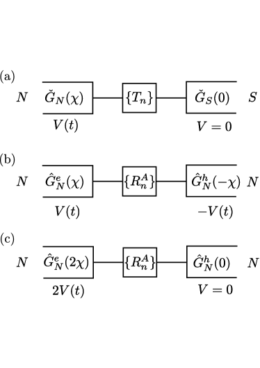
Figure 1: An Andreev contact (a) with transmission probabilities $\{T_{n}\}$ between a normal and a superconducting metal is mapped onto a contact (b) between two normal metals (electron and hole space), where the transmission probabilities are replaced by the Andreev reflection probabilities $\{R_{n}^{A}\}$. (c) By a further gauge transformation the counting field and the (time-dependent) voltage are applied on one side only.

At low energies, when $\check{G}_{S}$ is given by Eq. (8), the CGF reduces to the normal-state circuit with the electron and the hole Green’s functions:

$${\cal S}(\chi)=\frac{1}{2}{\rm Tr}\ln\left(1+\frac{R^{A}_{n}}{4}\Big{(}{\{\hat{G}_{N}^{e}(\chi),\hat{G}_{N}^{h}(-\chi)\}}-2\Big{)}\right).$$ (10)

Note that now $\hat{G}_{N}^{e,h}$ are the normal-state Green’s functions in the Keldysh space, and the transmission probabilities $T_{n}$ are replaced by Andreev reflection probabilities, $R^{A}_{n}=T_{n}^{2}/(2-T_{n})^{2}$. After carrying out a gauge transformation, it is possible to ascribe the counting field and the drive to one ’lead’ only, and we obtain

$${\cal S}(\chi)=\frac{1}{2}{\rm Tr}\ln\left(1+\frac{R^{A}_{n}}{4}\Big{(}{\{\hat{G}_{N}^{e}(2V(t),2\chi),\hat{G}_{N}^{h0}\}}-2\Big{)}\right),$$ (11)

where $\hat{G}_{N}^{h0}=\hat{G}_{N}^{h}(V=0,\chi=0)$. Thus, at the subgap energies, the system can be mapped to a normal-state circuit with a doubled voltage drive and a doubled counting field, and with transmission probabilities $T_{n}$ replaced by $R^{A}_{n}$. This mapping is shown in Fig. 1.

CGF in Eq. (11) can further be brought in the form:

$${\cal S}(\chi)= {\rm Tr}\ln\Big{[}1+(1-\tilde{f})fR^{A}_{n}(e^{2i\chi}-1)$$

$$+\tilde{f}(1-f)R^{A}_{n}(e^{-2i\chi}-1)\Big{]},$$ (12)

where $\tilde{f}=U^{2}\,f\,(U^{\dagger})^{2}$ accounts for an effective doubling of the drive voltage. At zero temperature the matrix operators $f$, $\tilde{f}$ have the additional property that $f^{2}=f$ and $\tilde{f}^{2}=\tilde{f}$, which allows us to decompose the FCS into the single electron processes and electron-hole pairs as mentioned in the introduction. Here in the Andreev case they take a slightly different form

$${\cal S}_{1} =\frac{2e{V_{\rm dc}}t_{0}}{h}\sum_{n}\ln\left[1+R^{A}_{n}(e^{i2\chi}-1)\right],$$ (13)

$${\cal S}_{eh} =M\sum_{nk}\ln\left[1+2R^{A}_{n}(1-R^{A}_{n})p_{k}(\cos(2\chi)-1)\right].$$ (14)

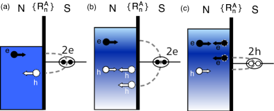
Figure 2: Elementary transport processes in a driven NS contact: (a) Andreev reflection of an excess electron due to dc voltage applied, see Eq. (13). (b) Andreev reflection of an electron from the electron-hole pair accompanied by the normal reflection of the hole from the pair, see Eq. (14). A reverse process is also possible in which the hole exhibits Andreev reflection and the electron exhibits normal reflection. Electrons and holes are defined relative to the energy of the superconducting condensate (${\epsilon}=0$). Time-dependent drive is indicated by shading.

CGF in Eq. (13) accounts for the Andreev reflection of the excess electrons due to dc voltage applied, cf. Fig. 2(a). The charges are transferred in pairs and the statistics is binomial in each transport channel with the transmission probabilities given by the Andreev reflection coefficients $R^{A}_{n}$. The rate $2e{V_{\rm dc}}/h$ with which the excess electrons impinge on the contact is the same as in the normal case. CGF in Eq. (14) accounts for the charge transfer statistics due to electron-hole pairs created by the ac drive. In general, ${\cal S}_{eh}$ consists of two types of electron-hole processes with different probabilities $p_{k}$ of the electron-hole pair creations and different numbers of attempts for particles to traverse the junction, $M=(\hbar\omega t_{0}/h)(1-v)$ and $M=(\hbar\omega t_{0}/h)v$. Here, $v=2e{V_{\rm dc}}/\hbar\omega-\lfloor 2e{V_{\rm dc}}/\hbar\omega\rfloor$ is a fractional part of $2e{V_{\rm dc}}/\hbar\omega$ ($\lfloor x\rfloor$ denotes the integer part of $x$). Charge transfers described by Eq. (14) are bidirectional processes in which an electron from the pair is Andreev reflected at the contact while the hole exhibits a normal reflection, or vice versa. This is schematically depicted in Fig. 2(b). As a result, pairs of charge quanta are transferred in either direction with the probabilities $R^{A}_{n}(1-R^{A}_{n})p_{k}$ in each transport channel.

4 Andreev levitons in an NS junction

Figure 3: Lorentzian voltage pulses for different widths: $\tau_{L}/T=0.05$ (dash-dotted), $0.1$ (solid), and $0.2$ (dashed line).

As a first example we compute the photon-assisted noise when the junction is driven by periodic Lorentzian voltage pulses of the form:

$$V_{\rm Lor}(t) =\frac{V_{0}}{\pi}\sum_{k=-\infty}^{\infty}\frac{T\tau_{L}}{(t-kT)^{2}+\tau_{L}^{2}}$$

$$=\frac{V_{0}\sinh(2\pi\tau_{L}/T)}{\cosh(2\pi\tau_{L}/T)-\cos(2\pi t/T)}.$$ (15)

Here, $T=2\pi/\omega$ is the period of the drive, and the amplitude $V_{0}$ is chosen in such a way as to represent the average voltage per period, $(1/T)\int_{0}^{T}V_{\rm Lor}(t)dt=V_{0}$. Lorentzian voltage pulses are shown in Fig. 3 for different widths $\tau_{L}/T=0.05$, $0.1$, $0.2$.

The excess photon-assisted noise (the total noise minus dc noise level) is given by

$$\frac{S_{\rm ac}}{S_{0}}=\sum_{n=-\infty}^{\infty}\left|\frac{2eV_{0}}{\hbar\omega}+n\right|\,|a_{n}|^{2}-\left|\frac{2eV_{0}}{\hbar\omega}\right|,$$ (16)

where

$$S_{0}=\frac{4e^{2}\hbar\omega}{h}\sum_{n}R^{A}_{n}(1-R^{A}_{n}).$$ (17)

Coefficients $a_{n}$ are related to the doubled ac part of the drive voltage, $2V_{\rm ac}(t)=2(V_{\rm Lor}(t)-V_{0})$:

$$a_{n}=\frac{1}{T}\int_{0}^{T}dt\,e^{-i\phi(t)}\,e^{in\omega t},$$ (18)

where $\phi(t)=(e/\hbar)\int_{0}^{t}2V_{\rm ac}(t^{\prime})dt^{\prime}$. These coefficients read [35]:

$$a_{n}=q\gamma^{n}\sum_{k=0}^{\infty}\frac{(-1)^{k}\,\gamma^{2k}\,\Gamma(q+n+k)}{\Gamma(k+1)\Gamma(q-k+1)\Gamma(n+k+1)}$$ (19)

for $n\geq 0$, and

$$a_{n}=q\gamma^{|n|}\sum_{k=0}^{\infty}\frac{(-1)^{k+n}\,\gamma^{2k}\,\Gamma(q+k)}{\Gamma(k+1)\Gamma(q-|n|-k+1)\Gamma(|n|+k+1)}$$ (20)

for $n<0$. Here, $q=2eV_{0}/\hbar\omega$ and $\gamma=e^{-2\pi\tau_{L}/T}$.

The photon-assisted noise is shown in Fig. 4(a). As the width $\tau_{L}$ is increased, the pulses overlap more strongly and $V_{\rm Lor}(t)$ approaches the constant voltage $V_{0}$. This results in the overall suppression of the excess photon-assisted noise. In addition, the excess noise is fully suppressed at half-integer values of $eV_{0}/\hbar\omega$. This corresponds to the half-integer Lorentzian pulses $e\int V_{\rm Lor}(t)dt=nh/2$, in contrast to the normal junctions in which the noise suppression occurs for integer pulses.

Figure 4: (a) Excess photon-assisted noise due to a Lorentzian voltage drive shown in Fig. 3 and (b) the corresponding probabilities of the electron-hole pair creations as a function of the drive amplitude.

The photon-assisted noise can also be expressed in terms of elementary events of the electron-hole pair creations [21, 22]:

$$S_{\rm ac}/S_{0}=2(1-v)\sum_{k}p_{k}.$$ (21)

Here, $v=2eV_{0}/\hbar\omega-\lfloor 2eV_{0}/\hbar\omega\rfloor$ is the fractional part of $2eV_{0}/\hbar\omega$ and $p_{k}$ are the probabilities of the pair creations given by $p_{k}=\sin^{2}(\alpha_{k}/2)$ where $e^{\pm i\alpha_{k}}$ are the eigenvalues of the operator $h\tilde{h}$. The electron-hole creation probabilities as a function of the amplitude of the Lorentzian pulses are shown in Fig. 4(b). We find that in the problem at hand, there is only one electron-hole pair created per period with probability $p_{1}\equiv p$. The pair creation probability increases as $eV_{0}/\hbar\omega$ approaches the half-integer values. However, the photon-assisted noise is nevertheless zero at these points because the effective rate of attempts $\hbar\omega(1-v)/h$ vanishes.

5 Large excitation noise

In what follows we allow for the dc bias and the ac drive amplitudes to be comparable to $\Delta$. For simplicity, we still assume low-temperature limit, $T_{e}=0$.

When the drive amplitudes are comparable to $\Delta$, the NS junction can no longer be mapped to the normal one. However, we can proceed with the numerical calculation of the cumulant generating function in Eq. (9). The Green’s functions are given by

$$\check{G}_{N}(0) =\begin{pmatrix}\bar{\tau}_{3}&2\bar{h}\\ 0&-\bar{\tau}_{3}\end{pmatrix},$$ (22)

$$\check{G}_{S}(0) =\begin{pmatrix}\bar{G}_{R}&(\bar{G}_{R}-\bar{G}_{A})h({\epsilon})\\ 0&\bar{G}_{A}\end{pmatrix}.$$ (23)

Here,

$$\bar{h}=\begin{pmatrix}h_{1}&0\\ 0&-h_{2}\end{pmatrix},$$ (24)

$$\bar{G}_{R,A}=\frac{\pm 1}{\sqrt{({\epsilon}\pm i0)^{2}-\Delta^{2}}}\begin{pmatrix}{\epsilon}\pm i0&\Delta\\ -\Delta&-({\epsilon}\pm i0)\end{pmatrix},$$ (25)

and $h_{1}=UhU^{\dagger}$, $h_{2}=U^{\dagger}hU$.

Next, we note that for the periodic time-dependent drive with the period $T=2\pi/\omega$, the operators $h_{1,2}$ couple only the energies that differ by an integer multiple of $\hbar\omega$. Therefore we can use a matrix representation in energy indices, $(h_{i})_{nm}(\epsilon)=h_{i}(\epsilon+n\hbar\omega,\epsilon+m\hbar\omega)$ ($-\hbar\omega/2<\epsilon<\hbar\omega/2$). This provides a matrix structure in energy in $\check{G}_{N}$ and $\check{G}_{S}$. The trace operation in Eq. (9) now amounts to a matrix diagonalization in Keldysh, Nambu, and energy indices and integration over $\epsilon$.

We calculate the cumulant generating function for a diffusive NS junction that has a distribution of transmission eigenvalues given by

$$\rho(T)=\frac{G_{N}}{G_{Q}}\frac{1}{2T\sqrt{1-T}},$$ (26)

where $G_{N}$ is the normal-state conductance and $G_{Q}=2e^{2}/h$ and it is assumed that the Thouless energy is much larger than all other relevant energy scales. The cumulant generating function in Eq. (9) reduces to

$${\cal S}(\chi)=-\frac{G_{N}}{2G_{Q}}{\rm Tr}\arcsin^{2}\left(\frac{1}{2}\sqrt{2-{\{\check{G}_{N}(\chi),\check{G}_{S}\}}}\right).$$ (27)

For the average current and the current noise power we obtain

$$I=G_{N}\int_{-\hbar\omega/2}^{\hbar\omega/2}\frac{d\epsilon}{4e}\sum_{\lambda}\frac{\partial\arcsin^{2}(\sqrt{\lambda(\epsilon,\chi)}/2)}{\partial(i\chi)}\Big{|}_{0},$$ (28)

$$S=-G_{N}\int_{-\hbar\omega/2}^{\hbar\omega/2}\frac{d\epsilon}{4}\sum_{\lambda}\frac{\partial^{2}\arcsin^{2}(\sqrt{\lambda(\epsilon,\chi)}/2)}{\partial(i\chi)^{2}}\Big{|}_{0},$$ (29)

where $\lambda$ are the eigenvalues of $2-{\{\check{G}_{N}(\chi),\check{G}_{S}\}}$.

Photon-assisted noise $S_{\rm ac}=S-S_{\rm dc}$ for an NS junction driven by periodic Lorentzian pulses is shown in Fig. 5 for different drive frequencies $\hbar\omega/\Delta=0.25$, $0.2$, $0.15$, $0.1$, $0.02$ (top to bottom). The noise is normalized to $S_{0}$ in Eq. (17) which in the case of a diffusive junction reads $S_{0}=G_{N}\hbar\omega/3$.

Figure 5: Excess photon-assisted noise for the Lorentzian pulses with $\tau_{L}/T=0.1$. The noise is shown for different drive frequencies: $\hbar\omega/\Delta=0.25$, $0.20$, $0.15$, $0.10$, $0.02$ (top to bottom).

The half-integer Lorentzian pulses with $eV_{0}/\hbar\omega=n/2$ at energies much smaller than the superconducting gap create Andreev levitons which are the minimal excitation states of the NS system. As the energy becomes comparable to the gap, the system can no longer be mapped to an effective normal junction. Therefore, the half-integer Lorentzian pulses are no longer optimal due to contributions of normal and Andreev electron transport above the gap. As a result, the excess photon assisted noise starts to increase, see Fig. 5. However, at energies much larger than the gap, the junction is in the normal state and the integer Lorentizan pulses create minimal excitation states in the normal junction.

Figure 6: Excess photon-assisted noise for the harmonic time-dependent voltage $V(t)=V_{0}[1+\cos(\omega t)]$ and amplitudes of the drive that are (a) smaller and (b) larger than the gap. At subgap energies the excess noise is minimal at half-integer drive amplitudes $eV_{0}/\hbar\omega=n/2$, while above the gap it is minimal at integer drive amplitudes $eV_{0}/\hbar\omega=n$.

The quantum oscillations of the photon assisted noise as a function of the dc voltage have been observed recently in the normal-state tunnel junction driven by harmonic time-dependent voltage $V(t)=V_{0}[1+\cos(\omega t)]$ [26]. Harmonic drive in general creates additional electron-hole pairs which results in the non-zero excess noise with minima at integer values $eV_{0}/\hbar\omega=n$. The same is true in the NS junction at energies much lower than the gap, except that the excess noise minima appear at half-integer values $eV_{0}/\hbar\omega=n/2$, see Fig. 6. At intermediate drive frequencies that are comparable to the gap, the noise in the system is determined by a density of states which is affected both by the drive and by the superconducting proximity effect. In addition, both normal and Andreev processes contribute to the transport. As a result, the total noise can even be suppressed below the effective dc noise level (the excess noise can be negative), the situation which otherwise cannot occur in the normal junction.

6 Conclusion

We have analyzed the transport properties of a driven quantum point contact between a normal metal and a superconductor. Using an extended Keldysh Greens function method we could determine the full counting statistics and identify the elementary transport processes for an arbitrary voltage drive in the subgap regime. At voltage amplitudes and frequencies well below the superconducting gap $\Delta$ the NS-contact can be mapped onto a contact with two normal leads. The transmission is determined by the Andreev reflection probability and the probabilities of elementary Andreev processes are determined by the ones known for normal transport with an effective charge $2e$. In that spirit we have discussed Lorentzian voltage pulse which lead to Andreev-Levitons, which are now pure two-charge excitations, for half-integer quantized amplitudes $e\int dtV=nh/2$. Finally we have discussed the transition from half-integer steps $eV_{0}/\hbar\omega=n/2$ in the ac-noise to simply quantized steps for voltages and frequencies much larger than $\Delta$.

In future it will be interesting to investigate open questions, e.g., for which parameters the noise is minimized and the nature of the elementary events at intermediate frequencies where both Andreev and normal reflection processes coexist, as well as the effects of dephasing related to the finite Thouless energy.

We acknowledge financial support by DFG through SFB 767 and BE3803/5. MV acknowledges the Serbian Ministry of Science Project No. 171027.

References

- [1] Y. M. Blanter, M. Büttiker, Shot noise in mesoscopic conductors, Physics Reports 336 (2000) 1.
- [2] W. Schottky, Über spontane stromschwankungen in verschiedenen elektrizitätsleitern, Ann. Phys. (Leipzig) 362 (1918) 541.
- [3] V. A. Khlus, Current and voltage fluctuations in microjunctions between normal metals and superconductors, Sov. Phys. JETP 66 (1987) 1243.
- [4] G. B. Lesovik, Excess quantum noise in 2D ballistic point contacts, JETP Lett. 49 (1989) 592.
- [5] M. Reznikov, M. Heiblum, H. Shtrikman, D. Mahalu, Temporal correlation of electrons: Suppression of shot noise in a ballistic quantum point contact, Phys. Rev. Lett. 75 (1995) 3340.
- [6] A. Kumar, L. Saminadayar, D. C. Glattli, Y. Jin, B. Etienne, Experimental test of the quantum shot noise reduction theory, Phys. Rev. Lett. 76 (1996) 2778.
- [7] C. W. J. Beenakker, M. Büttiker, Suppression of shot noise in metallic diffusive conductors, Phys. Rev. B 46 (1992) 1889.
- [8] A. H. Steinbach, J. M. Martinis, M. H. Devoret, Observation of hot-electron shot noise in a metallic resistor, Phys. Rev. Lett. 76 (1996) 3806.
- [9] M. Henny, S. Oberholzer, C. Strunk, C. Schönenberger, 1/3-shot-noise suppression in diffusive nanowires, Phys. Rev. B 59 (1999) 2871.
- [10] L. S. Levitov, G. B. Lesovik, Charge distribution in quantum shot noise, JETP Lett. 58 (1993) 230.
- [11] A. F. Andreev, Thermal conductivity of the intermediate state of superconductors, Sov. Phys. JETP 19 (1964) 1228.
- [12] C. J. Lambert, Generalized Landauer formulae for quasi-particle transport in disordered superconductors, J. Phys. Condens. Matter 3 (1991) 6579.
- [13] C. W. J. Beenakker, Quantum transport in semiconductor-superconductor microjunctions, Phys. Rev. B 46 (1992) 12841.
- [14] B. A. Muzykantskii, D. E. Khmelnitskii, Quantum shot noise in a normal-metal – superconductor point contact, Phys. Rev. B 50 (1994) 3982.
- [15] M. J. M. de Jong, C. W. J. Beenakker, Doubled shot noise in disordered normal-metal–superconductor junctions, Phys. Rev. B 49 (1994) 16070.
- [16] X. Jehl, M. Sanquer, R. Calemczuk, D. Mailly, Detection of doubled shot noise in short normal-metal/superconductor junctions, Nature 405 (2000) 50.
- [17] K. E. Nagaev, M. Büttiker, Semiclassical theory of shot noise in disordered superconductor–normal-metal contacts, Phys. Rev. B 63 (2001) 081301.
- [18] G. B. Lesovik, L. S. Levitov, Noise in an ac biased junction: Nonstationary aharonov-bohm effect, Phys. Rev. Lett. 72 (1994) 538.
- [19] M. H. Pedersen, M. Büttiker, Scattering theory of photon-assisted electron transport, Phys. Rev. B 58 (1998) 12993.
- [20] V. S. Rychkov, M. L. Polianski, M. Büttiker, Photon-assisted electron-hole shot noise in multiterminal conductors, Phys. Rev. B 72 (2005) 155326.
- [21] M. Vanević, Y. V. Nazarov, W. Belzig, Elementary events of electron transfer in a voltage-driven quantum point contact, Phys. Rev. Lett. 99 (2007) 076601.
- [22] M. Vanević, Y. V. Nazarov, W. Belzig, Elementary charge-transfer processes in mesoscopic conductors, Phys. Rev. B 78 (2008) 245308.
- [23] L.-H. Reydellet, P. Roche, D. C. Glattli, B. Etienne, Y. Jin, Quantum partition noise of photon-created electron-hole pairs, Phys. Rev. Lett. 90 (2003) 176803.
- [24] R. J. Schoelkopf, A. A. Kozhevnikov, D. E. Prober, M. J. Rooks, Observation of “photon-assisted” shot noise in a phase-coherent conductor, Phys. Rev. Lett. 80 (1998) 2437.
- [25] A. A. Kozhevnikov, R. J. Schoelkopf, D. E. Prober, Observation of photon-assisted noise in a diffusive normal metal-superconductor junction, Phys. Rev. Lett. 84 (2000) 3398.
- [26] G. Gasse, L. Spietz, C. Lupien, B. Reulet, Observation of quantum oscillations in the photoassisted shot noise of a tunnel junction, Phys. Rev. B 88 (2013) 241402.
- [27] H. W. Lee, L. S. Levitov, Estimate of minimal noise in a quantum conductor, arXiv:cond-mat/9507011.
- [28] D. A. Ivanov, H. W. Lee, L. S. Levitov, Coherent states of alternating current, Phys. Rev. B 56 (1997) 6839.
- [29] J. Dubois, T. Jullien, F. Portier, P. Roche, A. Cavanna, Y. Jin, W. Wegscheider, P. Roulleau, D. C. Glattli, Minimal-excitation states for electron quantum optics using levitons, Nature 502 (2013) 659.
- [30] T. Jullien, P. Roulleau, B. Roche, A. Cavanna, Y. Jin, D. C. Glattli, Quantum tomography of an electron, Nature 514 (2014) 603.
- [31] W. Belzig, Y. V. Nazarov, Full counting statistics of electron transfer between superconductors, Phys. Rev. Lett. 87 (2001) 197006.
- [32] M. Vanević, W. Belzig, Control of electron-hole pair generation by biharmonic voltage drive of a quantum point contact, Phys. Rev. B 86 (2012) 241306.
- [33] W. Belzig, P. Samuelsson, Full counting statistics of incoherent Andreev transport, Europhys. Lett. 64 (2003) 253.
- [34] J. Torrès, T. Martin, G. B. Lesovik, Effective charges and statistical signatures in the noise of normal metal-superconductor junctions at arbitrary bias, Phys. Rev. B 63 (2001) 134517.
- [35] J. Dubois, J. Thibaut, C. Grenier, P. Degiovanni, P. Roulleau, D. C. Glattli, Integer and fractional charge lorentzian voltage pulses analyzed in the frame of photon-assisted shot noise, Phys. Rev. B 88 (2013) 085301.