On Disentangling Initial Mass Function Degeneracies in Integrated Light

Abstract

The study of extragalactic integrated light can yield partial information on stellar population ages, abundances, and the initial mass function (IMF). The power-law slope of the IMF has been studied in recent investigations with gravity-sensitive spectral indicators that hopefully measure the ratio between KM dwarfs and giants. We explore two additional effects that might mimic the effects of the IMF slope in integrated light, the low mass cutoff (LMCO) and a variable contribution of light from the asymptotic giant branch (AGB). We show that the spectral effects of these three (IMF slope, LMCO, AGB strength) are very similar and very subtle compared to age-abundance effects. We illustrate parameter degeneracies and covariances and conclude that the three effects can be disentangled, but only in the regime of very accurate observations, and most effectively when photometry is combined with spectroscopy.

1 Introduction

Deriving astrophysical parameters from integrated-light observables is a widely accepted practice in the field of Galactic and extragalactic research. However, increasing evidence shows that single-burst, single-composition stellar populations oversimplify the underlying stellar systems (Gratton et al., 2012; Kaviraj et al., 2007). Additional parameters in the modelling process, such as: multiple burst-age stellar populations (Trager et al., 2000a, 2005; Goudfrooij et al., 2011), metallicity and helium abundance variation (Norris, 2004; Lee et al., 2005), initial mass function (IMF) variation (Weidner et al., 2013; Bekki, 2013; Chabrier et al., 2014), and chemical abundance variation (Dotter et al., 2007; Lee et al., 2009) were investigated in hopes of reconciling various contradictions between observation and theory. This group explored metallicity-compositeness by varying the abundance distribution function (ADF; d$M$/d[M/H]; the mass fraction of the stellar population at each [M/H]) effect in Tang et al. (2014, Paper I). The ADF shape is a gentle rise at low abundance, a peak, and a steeper fall-off at high abundance. By varying the widths of the ADFs we discovered “red lean” and “red spread” phenomena. “Red lean” means that a narrower ADF appears more metal-rich than a wide one, and “red spread” describes that the spectral difference between wide and narrow ADFs increases as the ADF peak is moved to more metal-rich values.

We continue to explore in this paper additional underexplored effects, this time ones that might endanger measurements of the IMF slope in integrated stellar population (SP) models. The IMF is of importance in stellar and extragalactic astronomy, affecting galaxy luminosity evolution, star formation, chemical evolution, and mass budget between normal and dark matter. The IMF regulates the mass distribution of the stellar population, and thus impacts the luminosity function, mass to light (M/L) ratio, and number of stellar remnants. However, direct IMF slope derivations that counts individual stars are limited by observational capabilities, uncertainties concerning the mass-luminosity relation, stellar evolution, dynamical evolution, binary fraction, and many other factors. Recently reemerged gravity-sensitive spectral lines (e.g., CaT, Na i, and Wing-Ford band) show bright future applications for indirectly estimating the IMF slopes of unresolved galaxies (Cenarro et al., 2003; van Dokkum & Conroy, 2010; Conroy & van Dokkum, 2012b). Gravity-sensitive spectral lines measure the dwarf/giant ratio. Our stance is that this ratio could be altered by effects other than the IMF slope.

First, a low-mass cut-off for the IMF (LMCO), exists in every set of SP models. It is the mass limit of stars included at the lower mass end — any star with mass smaller than this limit is assumed to have no contribution in the SP models. Often, the LMCO is a pragmatic choice dictated by the choice of stellar evolutionary isochrones that go into the SP models. It is readily appreciated that the LMCO is closely related to the fraction of low mass stars, and thus the dwarf/giant ratio. Therefore, we may encounter degeneracy when determining IMF slope and LMCO simultaneously. The LMCO is variable among different SP models found in the literature. For example, the Padova isochrones (Bertelli et al., 2008, 2009) set 0.15 $M_{\odot}$ as the LMCO, while the composite isochrones of Conroy & van Dokkum (2012a) sets 0.08 $M_{\odot}$ as the LMCO. As a result, the derived IMF slope values may change when swapping between SP models.

Second, we note the possibility that the dwarf/giant ratio may come as easily from modulating the number of giants as modulating the number of dwarfs. The bolometrically brightest giants are asymptotic giant branch (AGB) stars. These evolved stars have long been known to be difficult to constrain in most SP models (Conroy & Gunn, 2010; Girardi et al., 2010, 2013) due to uncertain stellar evolution (in turn due to uncertain rules about mass loss in giants) and also difficult to empirically constrain due to counting statistics (Frogel et al., 1990; Santos & Frogel, 1997; Bruzual & Charlot, 2003; Salaris et al., 2014). We suggest a plausible, hypothetical trend, ADF-AGB-IMF masquerading, in which increased metallicity causes cooler giants, which causes increased mass-loss, which causes fewer AGB stars, which resembles an increase in IMF slope.

In this paper, we study spectral and photometric variations in response to simultaneous changes of IMF slope, LMCO, and AGB strength ($\S$2). We show that the degeneracies can be marginally lifted for old, metal-rich populations, but the degeneracies are still firm in young populations ($\S$2.2 & $\S$2.3). Next, we dig into the mechanisms behind all these variations by studying the numbers of stars, luminosities, colors, and spectral indices of each evolutionary phase ($\S$2.4).

Bottom-heavy IMFs are indicated in local massive and metal-rich elliptical galaxies (Cenarro et al., 2003; van Dokkum & Conroy, 2010; Conroy & van Dokkum, 2012b; Cappellari et al., 2012). On the other hand, star-formation theories such as Larson (1998, 2005) and Marks et al. (2012) imply the metal-free early Universe favors a top-heavy IMF. Weidner et al. (2013) points out a time-independent bottom-heavy IMF generates too little metal and fewer stellar remnants than observed. The hypothesis that IMF steepens as the Universe evolves will change the light ratio between metal-poor and metal-rich stars in a similar way as the ADF effect, thus we call here ADF-IMF coupling. In $\S$3, we build rough models with ADF-IMF coupling to explore the ramifications, at least qualitatively. The coupled models appear more metal-rich than the noncoupled models, due to the suppression of metal-poor stars, resembling the red lean effect.

Finally, we test parameter recovery using a Monte Carlo approach. The mean recovered values agree with the input values inside the error range without alarming systematics ($\S$4.4). We uncover covariances among the IMF slope, LMCO, and AGB effects when combined with the more usual age and metallicity effects. Though the magnitudes of the IMF-related effects are smaller than the latter effects, these two groups of effects vector almost orthogonally ($\S$4.3), and we prognosticate bright hopes for disentangling all of these stellar population parameters. A summary of our results are given in $\S$5.

2 IMF slope, LMCO, and AGB

2.1 Model description

A new version of old integrated-light models (Worthey, 1994; Trager et al., 1998) is adopted. The new models use a new grid of synthetic spectra in the optical (Lee et al., 2009) in order to address the effects of changing the detailed elemental composition on an integrated spectrum. The models retain single burst age and metallicity as parameters, but were expanded to also include metallicity-composite populations, and the three IMF-related parameters we discuss (IMF slope, LMCO, and AGB modulation).

For this work, we adopt the isochrones of Bertelli et al. (2008, 2009) using the thermally-pulsing asymptotic giant branch (TP-AGB) treatment described in Marigo et al. (2008). Improving upon Poole et al. (2010), stellar index fitting functions were generated from indices measured from the stellar spectral libraries of Valdes et al. (2004) as re-fluxed by I. Chilingarian (2014, private communication), Worthey et al. (2014a), MILES (Falcón-Barroso et al., 2011), and IRTF (Rayner et al., 2009), all transformed to a common 200 km s^-1 spectral resolution via smoothing if the spectral resolution was greater or by linear transformation after index measurement if the resolution was lesser. Index errors were assigned by iteratively comparing the libraries and seeking error models of the form $\sigma^{2}=\sigma^{2}_{\rm{floor}}+C\sigma^{2}_{\rm{photon}}$, where $\sigma_{\rm{floor}}$ is an error floor mostly applicable to indices of large wavelength span, and $C$ is a fitting constant. Multivariate polynomial fitting was done in five overlapping temperature swaths as a function of $\theta_{eff}$ = 5040/T_eff, log g, and [Fe/H]. The fits were combined into a lookup table for final use. As in Worthey (1994), an index was looked up for each bin in the isochrone and decomposed into “index” and “continuum” fluxes, which added, then re-formed into an index representing the final, integrated value after the summation.

The IMF slope, LMCO, and AGB effects are calculated at two representative values. The IMF slope is calculated at 2.35 and 1.70, the LMCO at 0.15 and 0.30 $M_{\odot}$, and the AGB contribution with full and 80% strength. For modeling, we define the AGB phase as beginning 0.5 mag brighter than the red clump, and continuing to the end of the star’s life. The number of AGB stars of each mass bin is reduced to 80% to simulate a weaker AGB strength model. The SP model with IMF slope of 2.35, LMCO of 0.15 $M_{\odot}$, and full AGB strength is chosen as the standard model. Parameter variations from these nominal values are carried with linear interpolation. Naturally, if the parameters drift too far from the modeled values they can no longer be considered realistic.

To illustrate the different effects we vary one parameter at a time. That is, the results we display graphically are partial derivatives ($\partial_{index}/\partial_{effect}$).

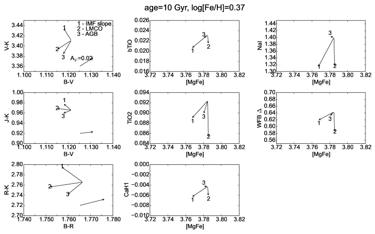
Figure 1: Color-color and index-index plots for an old, metal-rich population. The IMF slope, LMCO, AGB effects are labelled as vectors 1, 2, 3, respectively. At the bottom right of each plot involving photometric colors, an extinction vector of A${}_{V}=0.02$ mag is sketched.

2.2 An Old, Metal-rich Population

Since most of the elliptical galaxies in the local Universe are old and metal-rich, we pick age $=10$ Gy, and $\log(Z)=0.37$ to mimic a typical elliptical galaxy. In the left column of Figure 1, we show optical-near infrared (NIR) color-color plots. Note that we set the same y axis dynamic range (0.1 mag) for all the color-color plots. An extinction vector of A${}_{V}=0.02$ mag is sketched on the bottom right of each plots. We note that (1) the IMF slope, LMCO, and AGB effects are not parallel vectors, which means it is practical to lift the degeneracy of a single index with a mix of different colors. However, we note that these effects are detectable at the level of $\sim$0.02 mag. Such accuracies are comparable to contemporary detection limits and therefore technically challenging by today’s standards. In addition, (2) the ($J-K$) vs. ($B-V$) plot shows the weakest drifts among the three plots, due to the wavelength-proximity of these two pairs of filters. This wavelength-proximity is also the reason for small extinction vector. We also find that (3) decreasing the IMF slope and AGB strength tend to change the ($X-K$) colors in the opposite direction. Interestingly, increasing the LMCO leads to a decrease in ($V-K$) and ($R-K$), but an increase in ($J-K$), implying blue ($J-K$) colors for stars between 0.15 and 0.30 $M_{\odot}$ ($\S$2.4). (4) Finally, using colors alone, dust extinction is almost indistinguishable from LMCO effects.

In the middle and right columns of Figure 1, we plot [MgFe] versus five IMF-sensitive indices. We introduce to the Worthey models the optical IMF-sensitive indices bTiO and CaH1 from Spiniello et al. (2014), and plan to use them for future intermediate-redshift IMF research (Tang et al., in preparation). We notice that (1) the drifts caused by weakening the AGB strength are the smallest, due to low flux contribution of the AGB stars at the age of 10 Gyr ($\S$2.4). We also see that (2) decreasing the IMF slope tends to decrease the [MgFe] index (about 0.02 Å), while increasing the LMCO leads to small variation of [MgFe]. In addition, (3) the smaller dwarf/giant ratios induced by the IMF slope and LMCO effects lead to smaller values for IMF-sensitive indices. But the magnitude ratios of these two effects vary for different indices. The results that the LMCO drifts are larger than the IMF slope drifts in TiO2 and WFB $\Delta$ (Wing-Ford band) (Wing & Ford, 1969; Whitford, 1977; Hardy & Couture, 1988) suggest caution should be taken when interpreting these two indices as a clean IMF slope indicator.

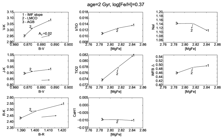
Figure 2: Color-color and index-index plots for a young, metal-rich population. The IMF slope, LMCO, AGB effects are labelled as vectors 1, 2, 3, respectively. At the bottom right of each color-color plot, an extinction vector of A${}_{V}=0.02$ mag is sketched.

2.3 A Young, Metal-rich Population

Schiavon et al. (2006) suggested young elliptical galaxies with ages of the order of 1 Gyr prevail in the early Universe (z$\sim$0.9). Studying these galaxies places important constraints on the elliptical evolution models. Here we pick age $=2$ Gyr, and $\log(Z)=0.37$ to mimic a young elliptical galaxy. In the all the plots of Figure 2, weakening the AGB strength induces a stronger drift than the old population, due to the high flux contribution of AGB stars at the age of $0.2-2$ Gyr (Maraston et al., 2006). To accommodate the large AGB drifts, the $y$ axis dynamic ranges are set to 0.25 mag for color-color plots. Note that this may causes visual differences between the color-colors plots of Figures 1 and 2.

In the optical-NIR color-color plots of Figure 2, (1) increasing the LMCO leads to negligible signal, while weakening the AGB strength shows a drift that is a factor of two larger as the old population. Another noticeable change is (2) the optical colors on $x$ axis. Instead of getting bluer as the old population does, decreasing the IMF slope of a young population drives the ($B-V$) and ($B-R$) colors redder, probably due to stronger post main sequence phases ($\S$2.4). Comparing with the extinction vectors, (3) the AGB drift and IMF slope drift should be clearly detectable at 0.02 mag level.

In the middle and right columns, (1) the index increases of bTiO, TiO2, and WFB $\Delta$ caused by decreasing the IMF slope of a young population confirm that IMF determination is sensitive to the age parameter. We also see that (2) the shallower IMF slope model also has greater [MgFe] than the standard model. In addition, (3) the AGB and IMF slope effects vector almost oppositely in most of the Figure 2 plots. The partial derivative nature of our results reveals the degeneracy of IMF slope and AGB strength is still firm for the young population. We further discuss the reasons for different drift directions by inspecting the luminosity weights, colors, and indices of each evolutionary phase in $\S$2.4.

2.4 Colors and Indices Broken into Evolutionary Phases

Table 1: Colors and Indices of Each Phase for the Old Population

		OLD POPULATION
	PHASE a	PHASE b	PHASE c	PHASE d
(B-V)	1.46939	0.69314	0.93189	1.48725
(V-K)	4.04228	1.75775	2.87041	4.84277
[MgFe]	3.77325	2.34650	2.83331	4.98660
bTiO	0.17246	-0.00274	0.00573	0.18546
TiO2	0.44303	0.01672	0.07097	0.33609
WFB $\Delta$	2.07944	0.06787	0.35408	1.16696

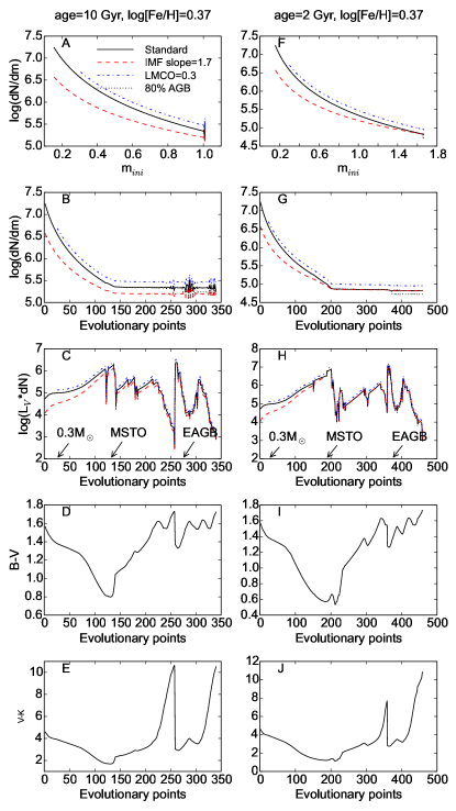
Figure 3: The number of stars, luminosities, and colors of the old, and young populations are plotted against isochrone evolutionary points or m_ini, where the use of evolutionary points better higlights post main-sequence phases. Four phases are defined as: phase $a$, $0.15<m_{ini}<0.30~{}M_{\odot}$; phase $b$, $m_{ini}=0.30~{}M_{\odot}$ to the main sequence turn-off (MSTO); phase $c$, from MSTO to the beginning of the AGB phase, or early AGB (EAGB); phase d, the AGB phase.

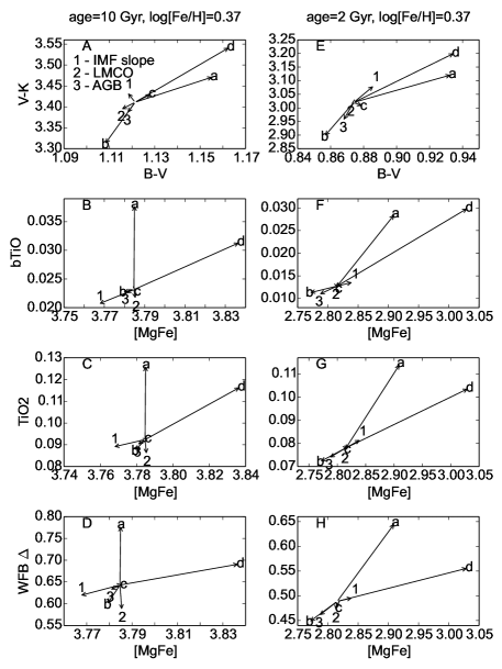
Figure 4: To illustrate the connections of effects and evolutionary phases, we connect the standard models with the contributions of each phase. The phase vectors (a,b,c,d) are shrunk to one tenth of the original magnitude to accommodate the three effect vectors. The vector of each phase is labelled by the corresponding phase name.

To illustrate the reasons behind the color drifts of three effects, we show the number of stars, luminosities, and colors in Figure 3. First, we take a look at the old population. In Figure 3A, we plot the logarithmic number of stars per initial mass ($\log(dN/dm)$) versus initial mass ($m_{ini}$). All stars with $m_{ini}\gtrsim 1.0~{}M_{\odot}$ have evolved to the stellar remnant phase, thus they do not contribute to the optical-NIR integrated light any more. The shallower IMF model has smaller $dN/dm$ than the standard model in the range of 0.15 to $\sim 1.0~{}M_{\odot}$, while the model with 0.3 $M_{\odot}$ LMCO has more stars in the range of 0.3 to$\sim 1.0~{}M_{\odot}$, due to a normalization correction (all stellar population are normalized to the same initial mass, so, for example, raising the LMCO means that more mass and more light is distributed to the stars that remain). The 80% AGB model is not discernible here, because the AGB stars have very small initial mass range ($\sim 1.0~{}M_{\odot}$). To inspect the strong variance of the post main sequence phases, we use the evolutionary points as $x$ variables instead of $m_{ini}$. The evolutionary points are defined as points with the same interval arc length along the isochrones in the HR diagram. Figure 3B clearly shows different number of stars for the standard model and the 80% AGB strength model. In Figure 3C, we find that the post main sequence stars, though small in number, have major contribution in the $V$ band integrated light. Then we plot the ($B-V$), and ($V-K$) colors in Figure 3D and 3E. Obviously, the very low mass stars and the giants have comparable ($B-V$) colors, but the giants, on average, show redder ($V-K$) colors.

To better quantify the contribution of different phases, we first define four phases: phase a, $0.15<m_{ini}<0.30~{}M_{\odot}$; phase b, $m_{ini}=0.30~{}M_{\odot}$ to the main sequence turn-off (MSTO); phase c, from MSTO to the beginning of the AGB phase, or early AGB (EAGB); phase d, the AGB phase. Next, we run the models with only one phase on by nullifying the contribution of all other phases. For example, to study the integrated light from phase a stars, we set the number of stars in phase b, c, and d to zero. The colors and indices from each phase are tabulated in Table 1. A vector that connects the standard model and one of these indices (or colors) indicates the drift direction if more stars in the corresponding phase are added. In Figure 4, these vectors are shrunk to one tenth of the original magnitude to accommodate the three drift vectors. In the ($V-K$) vs. ($B-V$) plot, the phase a vector is in the opposite direction of the LMCO drift, and similarly the phase d vector has an angle of almost 180 degrees with the AGB drift. These indicate the LMCO effect is mainly caused by decreasing the contribution of phase a stars, and the AGB effect is mainly caused by decreasing the contribution of phase d stars. These two conclusions might be obvious, but no vector seems directly related to the IMF slope drift. The IMF slope effect changes the number of stars of all masses, which means the high-to-low-mass ratio of each phase is not a constant. Therefore, we need to take the flux contribution of each phase into consideration. In Figure 5E, we plot the integrated optical spectra of four phases. The spectra of phase b and c are both luminous, although phase c stars become brighter than phase b stars as wavelength exceeds $\log(\lambda)\approx 3.65$ ($\approx$ 4467 Å). In Figure 5A, 5B, 5C, and 5D, we search for the spectral variation signals. The spectra of each phase are first normalized at $\log(\lambda)=3.815$. Then the spectrum of the shallower IMF model is divided by the standard model. The spectral ratios show shallower IMF model tends to blue the spectrum of phase b stars, but redden the spectrum of phase c stars. Therefore, the bluing and reddening effects compete again each other to determine the integrated color drifts, depending on the flux ratios of phase b stars to phase c stars (b/c) at different wavelengths. Let us take the ($B-V$) vs. ($V-K$) plot as an example. The b/c flux ratio is close to unity at the $B$ and $V$ bands, but much smaller than 1 at the K band. Thus the ($B-V$) color is governed almost equally by both the phase b stars and phase c stars, while the ($V-K$) color is mainly controlled by the phase c stars that redden the spectrum. The ($B-V$) color drifts blue due to the stronger spectral variation of phase b stars (Figure 5B) compared to phase c stars (Figure 5C).

In the index-index plots of Figure 4B, 4C, and 4D, similar conclusions as Figure 4A can be drawn for the LMCO and AGB drifts, based on the a and d vector directions. However, the index variations for the IMF slope effect cannot be easily determined from Figure 5. To better quantify the response of different phases, we show the index-index plots of all four phases in Figure 6. We notice the drift magnitudes of the phase b stars are much greater than the phase c stars. Since the smallest b/c flux ratio is about 0.5 (at WFB, Figure 5E), phase b stars dominate the index variation, pushing all the indices to lower values.

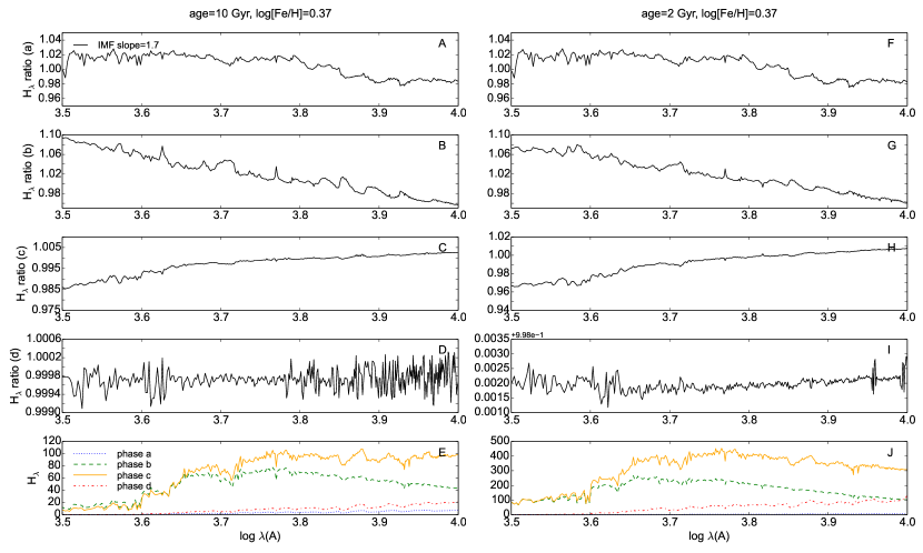
Figure 5: The upper four panels show the flux ratio between the shallower IMF models and the standard models, for four different phases. The very bottom panels plot the spectra of the standard models, subdivided into four phases.

Next, we switch to the young population. A major difference compared to the old population is that stars with mass between 1.0 to $\sim$1.66 M_⊙ still exist (Figure 3F). Two curves of different slopes intersect at $\sim$1.64 M_⊙, thus the shallower IMF model has more AGB stars than the standard model! Furthermore, Figure 3H shows longer post main sequence phases than the old population. In Figure 3I and 3J, we clearly see the MSTO hook features near the curve minimum. The hook feature happens when the star transitions from core burning to shell burning, with a brief gravitational-energy-dominated moment. The ($V-K$) color of the RGB tip is smaller than the old population, due to higher stellar mass and thus higher surface temperature of the RGB tip stars at young age. In Figure 4E, 4F, 4G, and 4H, the directions of vector a and d again testify the previous statement that the LMCO effect is mainly caused by phase a stars, while the AGB effect is mainly caused by phase d stars. To constrain the major contributor of the IMF slope effect, we plot the spectra and spectral ratios of all four phases in the right column of Figure 5. The spectrum of phase a is dwarfed by the flux increase of other three phases. Phase c is the most significant of all, starting to overcome phase b at $\log(\lambda)\approx 3.53$. As a result, phase c stars contribute most of the light in our optical, NIR colors and indices. Obviously, the spectral bluing and reddening competition of phase b and phase c stars (Figure 5 G and H) is won by the latter one, leading to redder ($B-V$) and ($V-K$) colors for shallower IMF slope. Comparison of the ($B-V$) color drifts of the old and young populations inspires us to search for the critical age where ($B-V$) color changes from drifting blue to drifting red. We find that the ($B-V$) colors of age less than 6 Gyr drift blue, but the ($B-V$) colors of age greater than 8 Gyr drift red. Therefore, between 6 Gyr and 8 Gyr, the main contributor of the IMF slope effect for ($B-V$) colors switches from phase b stars to phase c stars.

Before ending this section, we calculate the indices of each phase (Figure 7) to explain the IMF slope effects. The drift magnitude ratios of phase c over phase b stars has increased to about four times as the old population. Given that phase c stars dominate the flux contribution in most wavelength, bTiO, TiO2, WFB $\Delta$, and [MgFe] indices increase.

Figure 6: IMF slope drifts of each phase at old age.

Figure 7: IMF slope drifts of each phase at young age.

3 ADF-IMF coupling

To explore the ADF-IMF coupling, we built a toy model in which a hypothetical linear IMF$-$[M/H] relation is assumed. This linear relation is set by two points: $\alpha=2.35$ at $\log{\rm[M/H]}=0$, and $\alpha=1.35$ at $\log{\rm[M/H]}=-1$. Similar to Paper I, we employ CSPs with single-burst ages but normal-width composite abundance distribution functions (ADFs). Our normal-width ADF matches well the average solar neighborhood ADFs and Milky Way bulge ADFs in Paper I. To complete the models, the ADF-weighted Single Stellar Populations (SSPs) are combined to construct CSPs, in which the IMF slope of each mass bin matches the assumed IMF$-$[M/H] relation. To isolate the consequences of assuming a IMF$-$[M/H] relation, we also construct another CSP models with the normal-width ADF, but instead of assuming an IMF$-$[M/H] relation, we set the IMF to be always Salpeter ($\alpha=2.35$). We name the latter models Constant-IMF CSPs (CCSPs), and call the former models Variable-IMF CSPs (VCSPs). To verify the robustness of our models, we assemble observed elliptical galaxy spectra from Graves et al. (2007), Trager et al. (2008), and Serven (2010). Readers are referred to Paper I for sample descriptions. Note that all the model and observed indices are corrected to 300 km s^-1 resolution.

First, we take a look at the optical-NIR color-color plots (Figure 8A). The CCSPs and VCSPs are similar, but show differences, especially for the metal-poor populations. Since the photometric observations are not included in the above samples, we retrieve the ($B-V$) and ($V-K$) colors from Peletier (1989) and Persson et al. (1979).

1. Peletier (1989): In order to avoid focusing on only the cores of elliptical galaxies, we choose the colors at maximum isophotal radius. These colors are corrected for Galactic extinction before plotting.

2. Persson et al. (1979): We choose the well-tabulated ($B-V$) and ($V-K$) colors of field galaxies. These colors have been corrected for Galactic extinction in that paper.

In Fig. 8A the two photometric samples are divided into four bins in velocity dispersion ($<$150, 150$-$200, 200$-$250, $>$250 km s^-1) and we show the median colors of each bin as solid stars. These medians confirm that massive elliptical galaxies tend have redder ($V-K$) and ($B-V$) colors. Note that the ($V-K$) colors are only partially covered by the model grids. This model-observation mismatch might be partly because CSPs with peak [M/H]$>0.4$ is required, but we note that models with different isochrones (Worthey, 1994) have no trouble reaching red enough ($V-K$) colors. This is due to a slightly stronger coupling between metallicity and the temperature of the first-ascent giant branches in the older models. The ($V-K$) miss is almost certainly a model defect. We note that that flaw has little bearing on the results of this paper which are differential in character.

Figure 8B is the H$\beta-$[MgFe] plot, which is an age-metallicity diagnostic diagram. We apply nebular emission corrections for H$\beta$ to the Graves sample and Serven sample following the recipe of Serven & Worthey (2010). Five emission-corrected galaxies in the Serven sample are labelled as open triangles, since larger uncertainties might be expected for these galaxies in plots involving Balmer features. Generally speaking, the observational data points from the three samples locate at the old, metal-rich region, as what we expected.

Next, we pick several IMF-sensitive indices to study the model variations. Though the Serven sample and the Trager sample show moderate scatter compared with the model grids, it is encouraging to find the observed data from Graves et al. (2007) are well-covered by our models, and the variation trend looks reasonable.

In all the panels of Figure 8, we find that the VCSPs appear more metal-rich than the CCSPs. According to our IMF$-$[M/H] relation, the IMFs of the metal-poor populations in the VCSPs are shallower. We show that the shallower IMF model appear dimmer than the standard IMF model in Figure 3. Therefore, the metal-poor populations appear dimmer in the VCSPs. Note that metal-poor populations outshine their metal-rich counterparts, and thus the smaller integrated-light contribution from the metal-poor populations leads to more metal-rich appearing VCSPs.

Figure 8: The VCSPs (dashed lines) and CCSPs (solid lines) are described in 3. In the top left panel, measurements from Persson et al. (1979) (open pentagons), and Peletier (1989) (crosses) are shown. The medians of different velocity dispersions ($<$150, 150$-$200, 200$-$250, $>$250 km s^-1) are indicated as solid stars. In the optical index plots, Serven (triangles), Graves (open diamonds), and Trager (squares) observations are shown. Five Balmer emission galaxies in the Serven sample (open triangles) have had additional corrections applied.

4 Discussion

4.1 Swapping Models

To test the robustness of the model drifts, we also perform similar experiments with the Flexible Stellar Population Synthesis (FSPS, Conroy & Gunn 2010). We arranged to utilize the FSPS with the same age, IMF slope, and LMCO as our models. But the maximum metallicity of the Padova$+$MILES option is $\log$[Fe/H]$=0.20$, which is different than the metallicity we chose above (0.37). All the IMF-related spectral changes might be age and metallicity sensitive. Since the wavelength coverage of MILES is 3600$-$7400 Å, the Na i and WFB $\Delta$ are not available for analysis. To evaluate the AGB effect in FSPS, we choose the original Padova TP-AGB treatment (Marigo & Girardi, 2007) as the standard model, and compare it with the TP-AGB treatment of Conroy & Gunn (2010). Note that the latter TP-AGB treatment effectively reduces the NIR related colors at age around 1 Gyr, and well fits the colors of star clusters in the Magellanic Cloud (See their Figure 3). But both TP-AGB treatments have similar descriptions at old ages, and thus we expect small AGB drift for the old population in FSPS. This is different than the way we change the AGB strength in $\S$2.2: the AGB strength is always reduced to 80% of the full strength, regardless of the age.

We show the color-color plots and optical index-index plots in Figure 9 and 10. To compare with the results from our models, all the dynamic ranges are set to be the same as Figure 1 and 2. It is encouraging to find a lot of similarities in the directions and magnitudes of the drifts between two sets of models, but discrepancies still exist. For the old population, all the AGB drifts are very small, as expected. The IMF slope drifts seem smaller in the ($V-$K) colors, but show much bigger magnitudes in the negative [MgFe] direction. Note that the LMCO drift is no longer greater than the IMF slope drift for the TiO2 index: the IMF slope effect is the leading effect, now. Turning to the young population model, the color drifts of LMCO and IMF slope seem robust between two sets of models, but the AGB drifts are greater in the FSPS models, due to the strong reduction of TP-AGB stars around 1 Gyr. Surprisingly, the index drifts are much smaller than our models. This is possibly because of the different index derivation routines of these two model sets, but we are not sure of that.

Figure 9: Color-color and index-index plots at old age using FSPS models.

Figure 10: Color-color and index-index plots at young age using FSPS models.

4.2 Feasibility of Breaking the Degeneracy

Exploring whether the apparent steep IMF in massive elliptical galaxies might be partially due instead to the decreasing number of AGB stars requires one to be able to find an observational signature distinguish the two effects. We add to that list the LMCO, of course, but also note that various age and metallicity effects need to also be addressed, historically derived from the H$\beta-<$Fe$>$ or H$\gamma_{F}-<$Fe$>$ plot (Trager et al., 2000b, a; Tang et al., 2009).

For a young elliptical galaxy, the color-color plots of Figure 2 show substantial drifts ($\sim$0.03 mag) for the IMF slope and AGB effects. Note that the AGB and IMF slope effects vector oppositely in most of the Figure 2 plots . Since our results should be interpreted in a partial derivative sense, the opposite vectors in fact do nothing to disentangle the IMF slope and AGB effects. That is to say, the degeneracy is still firm and hard to break in this case.

But for an old, metal-rich galaxy, the color-color plots of Figure 1 show the LMCO, IMF slope, and AGB effects are distinguishable if the photometric accuracy is better than 0.02 mag. The index-index plots reveal robust IMF slope drift in the [MgFe] direction, reaching an amplitude of 0.02 Å. This separates the IMF slope effect from the LMCO effect, for the latter one causes much smaller drifts in the [MgFe] direction. Note that the [MgFe] index is insensitive to [$\alpha$/Fe], giving the [MgFe]-related plots advantage to different alpha-enhanced environment.

We find therefore that it is practical to lift the degeneracies using optical-red spectra and optical-NIR photometry if the measurements are accurate enough. We estimate these accuracies should be achieved: (1) dust attenuation $\sigma_{A_{V}}<$0.01 mag; (2) photometric accuracy $\sigma<$0.01 mag; (3) index accuracy $\sigma<$0.02 Å. As stellar photometric accuracy reaches milli-mag these days (Clem et al., 2007), an accuracy of 0.01 mag is feasible for nearby galaxies if one is precise about the observational complications. To list a few of them: dust attenuation, both Galactic and in-situ; sky subtraction for extended sources; aperture matching for spectroscopic and photometric extractions.

We also notice that the Na i index seems to be insensitive to the AGB effect for both the old and the young populations, in spite of Na i’s red central wavelength. A look at the index fitting functions at the stellar level reveals this insensitivity may relate to the similar Na i indices of giants and dwarfs. The Na i  index might be a way out of the ADF-AGB-IMF masquerading.

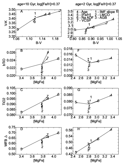
Figure 11: To visualize effects that may impact the SSP parameter determination, IMF slope, LMCO, AGB contribution, age, metallicity, ADF, and VCSP effects are labelled as vector 1 to 7, respectively.

4.3 Symposium of Multiple Effects

Age and metallicity effects are generally strong, but also degenerate in most of the colors and indices (Worthey, 1994). To obtain a bigger picture besides the three effects that we discuss in this paper, we summarize the effects concerning the IMF slope, LMCO, AGB contribution, age, metallicity, ADF, and VCSP in Figure 11. They are labelled as arrow 1 to 7, respectively. The parametrization of the first three effects is described in $\S$2.1. The age effect is estimated by calculating SP models of age$=$12 Gyr, $\log$[Fe/H]$=$0.37, and age$=$4 Gyr, $\log$[Fe/H]$=$0.37 ($\Delta$ age=$+2$ Gyr), while the metallicity effect is estimated by calculating SP models of age$=$10 Gyr, $\log$[Fe/H]$=$0.185, and age$=$2 Gyr, $\log$[Fe/H]$=$0.185 ($\Delta\log$[Fe/H]$=-0.185$). To investigate the effects concerning CSPs, we move the models with normal-width ADF, peak [M/H]$=0.4$, and constant IMF slope to the center. The ADF effect is shown as a displacement from the normal-width ADF CSPs to the narrow-width ADF CSPs, and the ADF-IMF coupling is represented by a vector from the CCSPs to the VCSPs.

Age and metallicity effects are parallel and degenerate as expected. They are joined by two new effects concerning the CSPs: the ADF and VCSP effects. In fact, the ADF effect is the same as the “red lean” effect (Paper I) where narrower ADF appears more metal-rich than a wider one. The reasons for the VCSP effect are explained in $\S$3. Careful readers may find that the ADF and VCSP effects both originate from the suppression of metal-poor populations, which leads to a metal-richer appearing integrated-light model. The similar origins and vector directions drive us to segregate the age, metallicity, ADF and VCSP effects into one group, and label them as group I effects. Group II effects are IMF slope, LMCO, and AGB contribution. Group II effects vector almost orthogonally to group I effects. Though group I effects are more prominent in magnitude, the orthogonality suggests that observations to isolate group II effects are still feasible.

4.4 Recovering [X/Fe], IMF slope, LMCO, and AGB Percentage

Worthey et al. (2014b) showed our efforts to recover elemental abundances from observed spectra. In this work, we upgrade our inversion program by replacing the SSP models with normal-width ADF CSP models and adding the IMF slope, LMCO, and AGB percentage (AGB%) parameter determination.

To examine the uncertainties of our inversion program, 500 mock galaxy spectra are constructed by Monte Carlo simulation. First, a model is produced with known age, abundance, IMF slope, LMCO, and AGB fraction. In this model the indices and colors are altered by random numbers which have a normal distribution. The standard deviation of the normal distribution function is set to 0.7$\sigma_{std}$, where $\sigma_{std}$ is a vector composed for reasonable guesses for the observational uncertainty in each color or index (Table 2). We supply the inversion program with each of these mock galaxy spectra in turn, and compare the recovered values with input values. Figure 12 show the recovered and input values of models at age = 12 Gyr, peak [M/H] = $-0.1$.

Table 2: Baseline Assumed Observational Uncertainty in Each Color or Index ($\sigma_{std}$)

	Index	$\sigma$	Unit		Index	$\sigma$	Unit		Index	$\sigma$	Unit		Index	$\sigma$	Unit
1	CN1	0.005	mag	24	H$\delta_{F}$	0.121	Å	47	Cr3594	0.131	Å	70	bTiOSTKC	0.005	mag
2	CN2	0.006	mag	25	H$\gamma_{F}$	0.114	Å	48	Cr4264	0.157	Å	71	aTiOSTKC	0.003	mag
3	Ca4227	0.081	Å	26	H$\alpha$	0.114	Å	49	Cr5206	0.077	Å	72	CaH1STKC	0.004	mag
4	G4300	0.155	Å	27	CO4685	0.339	Å	50	Mn3794	0.230	Å	73	CaH2STKC	0.003	mag
5	Fe4383	0.225	Å	28	CO5161	0.083	Å	51	Mn4018	0.325	Å	74	Na iSTKC	0.243	Å
6	Ca4455	0.128	Å	29	CNO3862	0.221	Å	52	Mn4061	0.147	Å	75	TiO2SDSS	0.003	mag
7	Fe4531	0.190	Å	30	CNO4175	0.285	Å	53	Mn4757	0.135	Å	76	H$\beta$emiss	0.090	Å
8	C24668	0.319	Å	31	Na8190	0.140	Å	54	Fe4058	0.173	Å	77	[O iii]emiss1	0.139	Å
9	H$\beta$	0.131	Å	32	Mg3835	0.156	Å	55	Fe4930	0.164	Å	78	[O iii]emiss2	0.091	Å
10	Fe5015	0.285	Å	33	Mg4780	0.156	Å	56	Co3701	0.135	Å	79	H$\beta_{0}$	0.159	Å
11	Mg1	0.003	mag	34	Si4101	0.096	Å	57	Co3840	0.142	Å	80	WFB $\Delta$	0.132	Å
12	Mg2	0.004	mag	35	Si4513	0.164	Å	58	Co3876	0.216	Å	81	($NUV-U$)	0.020	mag
13	Mgb	0.136	Å	36	Cahk	0.350	Å	59	Co7815	0.206	Å	82	($U-V$)	0.010	mag
14	Fe5270	0.151	Å	37	Ca8542	0.125	Å	60	Co8185	0.146	Å	83	($B-V$)	0.005	mag
15	Fe5335	0.172	Å	38	Ca8662	0.106	Å	61	Ni3667	0.215	Å	84	($V-I$)	0.005	mag
16	Fe5406	0.130	Å	39	Sc4312	0.115	Å	62	Ni3780	0.261	Å	85	($I-J$)	0.010	mag
17	Fe5709	0.106	Å	40	Sc6292	0.167	Å	63	Ni4292	0.131	Å	86	($I-K$)	0.010	mag
18	Fe5782	0.102	Å	41	Ti4296	0.112	Å	64	Ni4910	0.128	Å	87	($V-K$)	0.015	mag
19	NaD	0.127	Å	42	Ti4533	0.087	Å	65	Ni4976	0.116	Å	88	($I-L$)	0.020	mag
20	TiO1	0.003	mag	43	Ti5000	0.196	Å	66	Ni5592	0.117	Å	89	IRAC ($3.6-8.0$)	0.020	mag
21	TiO2	0.003	mag	44	V4112	0.282	Å	67	Ba4552	0.081	Å	90	WFC3 ($225w-555w$)	0.020	mag
22	H$\delta_{A}$	0.185	Å	45	V4928	0.097	Å	68	Ba4933	0.113	Å	91	($U-K$)	0.020	mag
23	H$\gamma_{A}$	0.195	Å	46	V6604	0.095	Å	69	Ba6142	0.100	Å	92	($NUV-K$)	0.020	mag

In Figure 12A, the age and peak [M/H] are quantized in the current inversion algorithm, since these two basic parameters are determined by closest-match rather than a smooth interpolation within the model grid. Age-metallicity degeneracy is the reason for the anti-correlation found in the first panel. In Figure 12B, we see tight correlation between [C/R] and [N/R], since these two elements are largely determined by common indices, the CN bands around 4100 Å. In Figure 12F, 12G, and 12H, the correlations among IMF slope, LMCO, and AGB% are generally loose. This implies the degeneracies among these three parameters are, for the most part, broken by our selection of indices. Though modest scatter exist in the recovered values, all of the mean recovered values agree with the input values inside the error range without alarming systematics. Some of the mean recovered values are especially close to the input values, e.g., IMF slope, [O/R] and [Na/R]. This success encourages us to apply our inversion program to observed galaxy spectra and colors in the future.

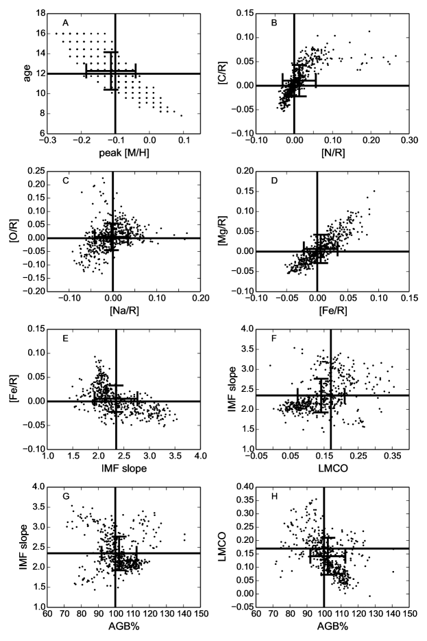
Figure 12: The recovered values (scattered dots) are compared with the input values (solid lines). The mean recovered values and their corresponding standard deviations are labelled with error bars.

5 Summary

A modeling study of various new parametric effects on integrated light, begun in Paper I by exploring the effects of the Abundance Distribution Function (ADF), continues on in this paper to explore two underexplored effects that might mimic IMF slope variation: the LMCO and the AGB strength. If we hypothesize that the apparently-steep IMF in massive elliptical galaxies might be partially due to the decreasing number of AGB stars, the question is can we ever know it, given the stellar population degeneracies. The magnitudes of the IMF slope, LMCO, and AGB effects are smaller than age and metallicity effects, but these two groups of effects vector almost orthogonally in diagnostic diagrams, which bodes well for measuring the combination of slope/LMCO/AGB effects. Internal to that trio, we explore the degeneracies and find that it is very difficult to distinguish steepening IMF from decreasing AGB strength for young, metal-rich populations. However, the slope/LMCO/AGB degeneracies can be lifted for old (age$\approx$10 Gyr), metal-rich populations using a combination of optical-to-near infrared photometry and spectroscopy. The disentanglement happens, however, at an observationally challenging level ($\approx$0.02 mag).

We fragmented our models into different evolutionary phases to isolate and discuss the leading factors for the IMF-related effects. We also investigated a series of models with an ADF-IMF coupling in which metal-rich populations favor low mass star formation. Models with ADF-IMF coupling appear more metal-rich than the noncoupled models, strongly resembling a modest narrowing of the ADF width, which has the same “red lean” effect. Attempting to recover the magnitude of an ADF-IMF coupling is very challenging from integrated light alone.

We upgraded our inversion program (Worthey et al., 2014b) by replacing the SSP models with normal-width ADF CSP models and adding the IMF slope, LMCO, and AGB percentage parameter determination. We estimated uncertainties on parameter estimation from Monte Carlo simulations, and find no significant systematic drifts, though of course we see many partial parameter degeneracies. The degeneracies among the IMF-related parameters can be broken by our selection of indices for old stellar populations. This success encourages us to seek appropriate observational material to apply our techniques to observed galaxy spectra and colors in the future.

6 Acknowledgements

The authors would like to thank I. Chilingarian for access to his improved version of the CFL library.

References

- Bekki (2013) Bekki K., 2013, Astrophys J., 779, 9
- Bertelli et al. (2008) Bertelli G., Girardi L., Marigo P., Nasi E., 2008, Astron. Astrophys., 484, 815
- Bertelli et al. (2009) Bertelli G., Nasi E., Girardi L., Marigo P., 2009, Astron. Astrophys., 508, 355
- Bruzual & Charlot (2003) Bruzual G., Charlot S., 2003, Monthly Notices Royal Astron. Soc., 344, 1000
- Cappellari et al. (2012) Cappellari M., McDermid R. M., Alatalo K., Blitz L., Bois M., Bournaud F., Bureau M., Crocker A. F., Davies R. L., Davis T. A., de Zeeuw P. T., Duc P.-A., Emsellem E., Khochfar S., Krajnović D., Kuntschner H., Lablanche P.-Y., Morganti R., Naab T., Oosterloo T., Sarzi M., Scott N., Serra P., Weijmans A.-M., Young L. M., 2012, Nature, 484, 485
- Cenarro et al. (2003) Cenarro A. J., Gorgas J., Vazdekis A., Cardiel N., Peletier R. F., 2003, Monthly Notices Royal Astron. Soc., 339, L12
- Cervantes & Vazdekis (2009) Cervantes J. L., Vazdekis A., 2009, Monthly Notices Royal Astron. Soc., 392, 691
- Chabrier et al. (2014) Chabrier G., Hennebelle P., Charlot S., 2014, Astrophys J., 796, 75
- Clem et al. (2007) Clem J. L., Vanden Berg D. A., Stetson P. B., 2007, Astron. J., 134, 1890
- Conroy & Gunn (2010) Conroy C., Gunn J. E., 2010, Astrophys J., 712, 833
- Conroy & van Dokkum (2012a) Conroy C., van Dokkum P., 2012a, Astrophys J., 747, 69
- Conroy & van Dokkum (2012b) Conroy C., van Dokkum P. G., 2012b, Astrophys J., 760, 71
- Dotter et al. (2007) Dotter A., Chaboyer B., Ferguson J. W., Lee H.-c., Worthey G., Jevremović D., Baron E., 2007, Astrophys J., 666, 403
- Falcón-Barroso et al. (2011) Falcón-Barroso J., Sánchez-Blázquez P., Vazdekis A., Ricciardelli E., Cardiel N., Cenarro A. J., Gorgas J., Peletier R. F., 2011, Astron. Astrophys., 532, A95
- Frogel et al. (1990) Frogel J. A., Mould J., Blanco V. M., 1990, Astrophys J., 352, 96
- Girardi et al. (2013) Girardi L., Marigo P., Bressan A., Rosenfield P., 2013, Astrophys J., 777, 142
- Girardi et al. (2010) Girardi L., Williams B. F., Gilbert K. M., Rosenfield P., Dalcanton J. J., Marigo P., Boyer M. L., Dolphin A., Weisz D. R., Melbourne J., Olsen K. A. G., Seth A. C., Skillman E., 2010, Astrophys J., 724, 1030
- González (1993) González J. J., 1993, PhD thesis, Thesis (PH.D.)–UNIVERSITY OF CALIFORNIA, SANTA CRUZ, 1993.Source: Dissertation Abstracts International, Volume: 54-05, Section: B, page: 2551.
- Goudfrooij et al. (2011) Goudfrooij P., Puzia T. H., Kozhurina-Platais V., Chandar R., 2011, Astrophys J., 737, 3
- Gratton et al. (2012) Gratton R. G., Carretta E., Bragaglia A., 2012, Astron. Astrophys. Review, 20, 50
- Graves et al. (2007) Graves G. J., Faber S. M., Schiavon R. P., Yan R., 2007, Astrophys J., 671, 243
- Hardy & Couture (1988) Hardy E., Couture J., 1988, Astrophys J. Letters, 325, L29
- Kaviraj et al. (2007) Kaviraj S., Kirkby L. A., Silk J., Sarzi M., 2007, Monthly Notices Royal Astron. Soc., 382, 960
- La Barbera et al. (2013) La Barbera F., Ferreras I., Vazdekis A., de la Rosa I. G., de Carvalho R. R., Trevisan M., Falcón-Barroso J., Ricciardelli E., 2013, Monthly Notices Royal Astron. Soc., 433, 3017
- Larson (1998) Larson R. B., 1998, Monthly Notices Royal Astron. Soc., 301, 569
- Larson (2005) —, 2005, Monthly Notices Royal Astron. Soc., 359, 211
- Lee et al. (2009) Lee H.-c., Worthey G., Dotter A., Chaboyer B., Jevremović D., Baron E., Briley M. M., Ferguson J. W., Coelho P., Trager S. C., 2009, Astrophys J., 694, 902
- Lee et al. (2005) Lee Y.-W., Joo S.-J., Han S.-I., Chung C., Ree C. H., Sohn Y.-J., Kim Y.-C., Yoon S.-J., Yi S. K., Demarque P., 2005, Astrophys J. Letters, 621, L57
- Maraston et al. (2006) Maraston C., Daddi E., Renzini A., Cimatti A., Dickinson M., Papovich C., Pasquali A., Pirzkal N., 2006, Astrophys J., 652, 85
- Marigo & Girardi (2007) Marigo P., Girardi L., 2007, Astron. Astrophys., 469, 239
- Marigo et al. (2008) Marigo P., Girardi L., Bressan A., Groenewegen M. A. T., Silva L., Granato G. L., 2008, Astron. Astrophys., 482, 883
- Marks et al. (2012) Marks M., Kroupa P., Dabringhausen J., Pawlowski M. S., 2012, Monthly Notices Royal Astron. Soc., 422, 2246
- Norris (2004) Norris J. E., 2004, Astrophys J. Letters, 612, L25
- Peletier (1989) Peletier R. F., 1989, PhD thesis, , University of Groningen, The Netherlands, (1989)
- Persson et al. (1979) Persson S. E., Frogel J. A., Aaronson M., 1979, Astrophys J. Supplement Series, 39, 61
- Poole et al. (2010) Poole V., Worthey G., Lee H.-c., Serven J., 2010, Astron. J., 139, 809
- Rayner et al. (2009) Rayner J. T., Cushing M. C., Vacca W. D., 2009, Astrophys J. Supplement Series, 185, 289
- Salaris et al. (2014) Salaris M., Weiss A., Cassarà L. P., Piovan L., Chiosi C., 2014, Astron. Astrophys., 565, A9
- Salpeter (1955) Salpeter E. E., 1955, Astrophys J., 121, 161
- Santos & Frogel (1997) Santos Jr. J. F. C., Frogel J. A., 1997, Astrophys J., 479, 764
- Schiavon et al. (2006) Schiavon R. P., Faber S. M., Konidaris N., Graves G., Willmer C. N. A., Weiner B. J., Coil A. L., Cooper M. C., Davis M., Harker J., Koo D. C., Newman J. A., Yan R., 2006, Astrophys J. Letters, 651, L93
- Serven & Worthey (2010) Serven J., Worthey G., 2010, Astron. J., 140, 152
- Serven (2010) Serven J. L., 2010, PhD thesis, Washington State University
- Spiniello et al. (2014) Spiniello C., Trager S., Koopmans L. V. E., Conroy C., 2014, Monthly Notices Royal Astron. Soc., 438, 1483
- Tang et al. (2014) Tang B., Worthey G., Davis A. B., 2014, Monthly Notices Royal Astron. Soc., 445, 1538
- Tang et al. (2009) Tang B.-T., Gu Q.-S., Huang S., 2009, Research in Astronomy and Astrophysics, 9, 1215
- Trager et al. (2008) Trager S. C., Faber S. M., Dressler A., 2008, Monthly Notices Royal Astron. Soc., 386, 715
- Trager et al. (2000a) Trager S. C., Faber S. M., Worthey G., González J. J., 2000a, Astron. J., 120, 165
- Trager et al. (2000b) —, 2000b, Astron. J., 119, 1645
- Trager et al. (1998) Trager S. C., Worthey G., Faber S. M., Burstein D., González J. J., 1998, Astrophys J. Supplement Series, 116, 1
- Trager et al. (2005) Trager S. C., Worthey G., Faber S. M., Dressler A., 2005, Monthly Notices Royal Astron. Soc., 362, 2
- Valdes et al. (2004) Valdes F., Gupta R., Rose J. A., Singh H. P., Bell D. J., 2004, Astrophys J. Supplement Series, 152, 251
- van Dokkum & Conroy (2010) van Dokkum P. G., Conroy C., 2010, Nature, 468, 940
- Weidner et al. (2013) Weidner C., Ferreras I., Vazdekis A., La Barbera F., 2013, Monthly Notices Royal Astron. Soc., 435, 2274
- Whitford (1977) Whitford A. E., 1977, Astrophys J., 211, 527
- Wing & Ford (1969) Wing R. F., Ford Jr. W. K., 1969, Pub. Astron. Soc. Pacific, 81, 527
- Worthey (1994) Worthey G., 1994, Astrophys J. Supplement Series, 95, 107
- Worthey et al. (2014a) Worthey G., Danilet A. B., Faber S. M., 2014a, Astron. Astrophys., 561, A36
- Worthey et al. (2014b) Worthey G., Tang B., Serven J., 2014b, Astrophys J., 783, 20