Prospects and status of quark mass renormalization in three-flavour QCD

Abstract:

We present the current status of a revised strategy to compute the running of renormalized quark masses in QCD with three flavours of massless O(a) improved Wilson quarks. The strategy employed uses the standard finite-size scaling method in the Schrödinger functional and accommodates for the non-perturbative scheme-switch which becomes necessary at intermediate renormalized couplings as discussed in [1411.7648].

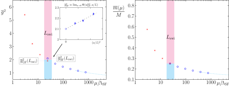
Figure 1: Sketch of the overall strategy to determine the $\Lambda$-parameter in $N_{\rm f}=3$ QCD (left) as well as the renormalization group running to invariant quark mass $M$ (right).

1 Introduction

In a mass-independent renormalization scheme for QCD, the renormalization group (RG) equations for the running coupling and quark mass read

$$\mu\dfrac{\partial}{\partial\mu}\overline{g}(\mu)=\beta(\overline{g}) \qquad\mathrel{\mathop{\sim}^{\overline{g}\to 0}}\qquad-\overline{g}^{3}({b_{0}}+{b_{1}}\overline{g}^{2}+{b_{2}}\overline{g}^{4}+\ldots)\;,$$ (1)

$$\mu\dfrac{\partial}{\partial\mu}\kern 1.0pt\overline{\kern-1.0ptm\kern-1.0pt}\kern 1.0pt(\mu)=\tau(\overline{g}) \qquad\mathrel{\mathop{\sim}^{\overline{g}\to 0}}\qquad-\overline{g}^{2}({d_{0}}+{d_{1}}\overline{g}^{2}+\ldots)\;,$$ (2)

with universal coefficients $b_{0},b_{1},d_{0}$ and higher order ones, $b_{i>1}$ and $d_{j>0}$, which are scheme-dependent. In such a scheme it is natural to first solve the RG equation for the coupling (1) and then for the mass (2), as the latter depends parametrically on the coupling only. Formally, the solutions can be exactly written down via renormalization group invariants (RGI),

$${\Lambda} \equiv\mu\big{[}{b_{0}\overline{g}^{2}(\mu)}\big{]}^{-{b_{1}}/({2b_{0}^{2}})}\,{\rm e}^{-1/({2b_{0}\overline{g}^{2}(\mu)})}\exp\bigg{\{}\!\!-\!\!\int_{0}^{\overline{g}^{\vphantom{A}}(\mu)}\!{\rm d}{g}\bigg{[}\dfrac{1}{\beta(g)}+\dfrac{1}{b_{0}g^{3}}-\dfrac{b_{1}}{b_{0}^{2}g}\bigg{]}\bigg{\}}\;,$$ (3)

$${M_{i}} \equiv\kern 1.0pt\overline{\kern-1.0ptm\kern-1.0pt}\kern 1.0pt_{i}(\mu)\big{[}{2b_{0}\overline{g}^{2}(\mu)}\big{]}^{-{d_{0}}/({2b_{0}})}\,\exp\bigg{\{}\!\!-\!\!\int_{0}^{\overline{g}^{\vphantom{A}}(\mu)}\!{\rm d}{g}\bigg{[}\dfrac{\tau(g)}{\beta(g)}-\dfrac{d_{0}}{b_{0}g}\bigg{]}\bigg{\}}\;,\quad i\in\{\rm u,d,s,c,b,t\}\,,$$ (4)

which encode all information about the respective fundamental parameters of QCD. They are defined without relying on perturbation theory, and, while the Lambda-parameter is trivially scheme-dependent, the RGI mass is independent of the renormalization scheme. Accordingly, the RGI parameters allow for easy conversion (at high but finite $\mu$) between renormalized masses or couplings in different (massless) schemes. The only remnant and non-trivial dependence is on the number of quark flavours $N_{\rm f}$. The RGIs $\{\Lambda,M_{i}\}_{N_{\rm f}}$ have been computed by the ALPHA collaboration in the past for $N_{\rm f}=0,2$ QCD, cf. Refs. [1, 2, 3, 4, 5]. In line with the current Coordinated Lattice Simulation effort (CLS) [6], a new computation has been started to determine the fundamental parameters $\{\Lambda,M_{i}\}_{N_{\rm f}}$ for QCD with $N_{\rm f}=3$ dynamical flavours. The standard techniques involved here have been refined over the years. As intermediate mass-independent renormalization scheme the Schrödinger functional (SF) is used with non-perturbatively improved Wilson fermions. In the SF the renormalization scale is given by the inverse box size $\mu=1/L$. Combined with a recursive finite-size scaling $L\to L/s$ in the continuum, typically with $s=2$, one can reach a scale difference of ${\rm O}(10^{3})$ after $N=10$ steps, and thus bridge the gap between typical large volume simulations $(L\sim 6\,{\rm fm})$ — where the scale has been set — and the regime where perturbation theory can be safely applied.

2 Revised strategy for $N_{\rm f}=3$

In order to achieve a precision on $\alpha_{\rm s}(M_{\rm Z})$ that is better than the current PGD estimate, the ALPHA collaboration has elaborated a new strategy which minimizes statistical and systematic effects by combining the standard SF coupling scheme with the new gradient flow (GF) sheme in the Schrödinger functional [7, 8]. To this end one has to match the two schemes non-perturbatively at some intermediate scale $\mu_{\rm swi}=1/L_{\rm swi}$, as indicated in the sketch shown in the left panel of Fig. 1 and explained in more detail at last year’s Lattice conference [9]. A status report has been given this year [10]. In Fig. 1 the red crosses indicate values for the gradient flow coupling $u^{\rm GF}=\overline{g}_{\rm GF}^{2}(L)$, $L\geq L_{\rm swi}$, which is used to make contact between a hadronic scale in large volumes, made available by CLS, and the switching scale $L_{\rm swi}$. From there on the Schrödinger functional coupling $u^{\rm SF}=\overline{g}_{\rm SF}^{2}(L)$, $L\leq L_{\rm swi}$, is used (blue circles) to make contact with perturbation theory (dashed curve) at very high energy in order to extract the $\Lambda$-parameter in physical units according to eq. (1).

$u^{\rm SF}$	$L/a$	$\beta$	${\kappa_{\rm crit}^{\rm SF}}$	$u^{\rm SF}_{\text{fit}}$
$1.1100$	$6$	$8.5403(55)$	$0.1323361(12)$	$1.1100(12)$
$1.1100$	$8$	$8.7325(72)$	$0.1321338(13)$	$1.1100(15)$
$1.1100$	$12$	$8.995(11)$	$0.1318617(10)$	$1.1100(24)$
$1.4808$	$6$	$7.2618(28)$	$0.1339337(13)$	$1.4808(11)$
$1.4808$	$8$	$7.4424(38)$	$0.1336745(11)$	$1.4808(15)$
$1.4808$	$12$	$7.7299(89)$	$0.13326299(69)$	$1.4808(35)$
$2.0120$	$6$	$6.2735(44)$	$0.1355713(17)$	$2.0120(32)$
$2.0120$	$8$	$6.4680(51)$	$0.1352362(15)$	$2.0120(39)$
$2.0120$	$12$	$6.7299(68)$	$0.1347591(10)$	$2.0120(49)$

Table 1: Simulation parameters and their known accuracy.

As aforementioned, solving the RG equation for the strong coupling is a prerequesite for solving other RG equations such as the one for the mass which we want to consider now. The general strategy for computing RGI quark masses follows the decomposition [4, 5]

$$M_{i} =\frac{M}{\kern 1.0pt\overline{\kern-1.0ptm\kern-1.0pt}\kern 1.0pt(\mu_{\rm had})}\times\kern 1.0pt\overline{\kern-1.0ptm\kern-1.0pt}\kern 1.0pt_{i}(\mu_{\rm had})\;, \mu_{\rm had} =1/L_{\rm had}\;,$$ (5)

where $L_{\rm had}$ is some hadronic scale of ${\rm O}(1\,{\rm fm})$ and the total RG running factor for the mass in the continuum, ${M}/{\kern 1.0pt\overline{\kern-1.0ptm\kern-1.0pt}\kern 1.0pt(\mu_{\rm had})}$, connects the renormalized current quark mass $\kern 1.0pt\overline{\kern-1.0ptm\kern-1.0pt}\kern 1.0pt_{i}(\mu_{\rm had})$ to its RGI value. This factor does not depend on the individual quark flavour $i\in\{{\rm u/d},{\rm s},{\rm c},{\rm b}\}$, and in the $N_{\rm f}=2$ case, with $\Delta[M/\kern 1.0pt\overline{\kern-1.0ptm\kern-1.0pt}\kern 1.0pt]=1.1\%$, it has been one of the dominant sources of errors in the determination of $M_{\rm s}$ [3] and $M_{\rm b}$ [11]. Accordingly, it is advisable to reduce this error systematically as much as possible in the forthcoming determination. Due to the recursive step-scaling procedure the total RG factor decomposes into

$$\dfrac{M}{\kern 1.0pt\overline{\kern-1.0ptm\kern-1.0pt}\kern 1.0pt(\mu_{\rm had})} =\dfrac{M}{\kern 1.0pt\overline{\kern-1.0ptm\kern-1.0pt}\kern 1.0pt(\mu_{\rm PT})}\times\prod^{N}_{i=1}{\sigma_{\rm P}(u_{i})}\;, u_{i} =\overline{g}^{2}(L_{\rm had}/2^{i})\,, \mu_{\rm PT} =2^{N}\mu_{\rm had}\,,$$ (6)

i.e., a product of step-scaling functions (SSF), $\sigma_{\rm P}(u_{i})$, and a part that can be safely evaluated in perturbation theory using eq. (4) after a sufficiently high scale $\mu_{\rm PT}$ is reached. The SSF reads

$${\sigma_{\rm P}(u_{i})} =\exp\!\bigg{[}-\!\int_{\overline{g}(\mu_{i})}^{\overline{g}(\mu_{i}/2)}\!\!\!\!{\rm d}{g}\,\dfrac{\tau(g)}{\beta(g)}\bigg{]}_{\overline{g}^{2}(\mu_{i})=u_{i}}^{m_{q}=0}=\lim_{a\to 0}\Sigma_{\rm P}(u_{i},a/L)\;, {\Sigma_{\rm P}(u_{i},a/L)} =\dfrac{{Z_{\rm P}}(g_{0},2L/a)}{{Z_{\rm P}}(g_{0},L/a)}\;,$$ (7)

i.e., it is obtained from its lattice SSF $\Sigma_{\rm P}$ along a line of constant physics (LCP) when $a\to 0$. This is achieved by implicitly prescribing a value $u_{i}$ to the renormalized coupling $\overline{g}^{2}$ in a given scheme at vanishing quark mass $m_{q}$. The relevant scale-dependent renormalization constant ${Z_{\rm P}}$ is obtained from standard correlation functions (${f_{\rm P}},{f_{1}}$) in the SF by the renormalization condition

$$\left[{{Z_{\rm P}}(g_{0},L/a)}\frac{{f_{\rm P}}(L/2)}{\sqrt{3{f_{1}}}}\right]_{m_{q}=0}^{\theta} =c_{3}(a/L)\;,$$ (8)

employing the known tree-level normalization $c_{3}(a/L)$ with vanishing boundary gauge fields and $(T/L,\theta,m_{q})=(1,0.5,0)$, cf. [4, 5]. For the three-flavour computation we are following as closely as possible the strategy for the running coupling, meaning that we also switch the scheme for setting up the LCP above/below $L_{\rm swi}$. The computation of the total RG factor is easily extended to this two-scheme case (GF/SF coupling) and reads

$$\dfrac{M}{\kern 1.0pt\overline{\kern-1.0ptm\kern-1.0pt}\kern 1.0pt(\mu_{\rm had})} =\dfrac{M}{\kern 1.0pt\overline{\kern-1.0ptm\kern-1.0pt}\kern 1.0pt(\mu_{\rm PT})}\times\dfrac{\kern 1.0pt\overline{\kern-1.0ptm\kern-1.0pt}\kern 1.0pt(\mu_{\rm PT})}{\kern 1.0pt\overline{\kern-1.0ptm\kern-1.0pt}\kern 1.0pt(\mu_{\rm swi})}\times\dfrac{\kern 1.0pt\overline{\kern-1.0ptm\kern-1.0pt}\kern 1.0pt(\mu_{\rm swi})}{\kern 1.0pt\overline{\kern-1.0ptm\kern-1.0pt}\kern 1.0pt(\mu_{\rm had})}\;, \mu_{\rm PT} =2^{N_{\rm SF}}\mu_{\rm swi}\,, \mu_{\rm swi} =2^{N_{\rm GF}}\mu_{\rm had}\,,$$ (9a)

with

$$\dfrac{\kern 1.0pt\overline{\kern-1.0ptm\kern-1.0pt}\kern 1.0pt(\mu_{\rm PT})}{\kern 1.0pt\overline{\kern-1.0ptm\kern-1.0pt}\kern 1.0pt(\mu_{\rm swi})} =\prod^{N_{\rm SF}}_{i=1}{\sigma_{\rm P}(u^{\rm SF}_{i})}\;, u^{\rm SF}_{i} =\overline{g}_{\rm SF}^{2}(L_{\rm swi}/2^{i})\,,$$ (9b)

$$\dfrac{\kern 1.0pt\overline{\kern-1.0ptm\kern-1.0pt}\kern 1.0pt(\mu_{\rm swi})}{\kern 1.0pt\overline{\kern-1.0ptm\kern-1.0pt}\kern 1.0pt(\mu_{\rm had})} =\prod^{N_{\rm GF}}_{i=1}{\sigma_{\rm P}(u^{\rm GF}_{i})}\;, u^{\rm GF}_{i} =\overline{g}_{\rm GF}^{2}(L_{\rm had}/2^{i})\,.$$ (9c)

By doing so we directly profit from the running coupling project [9, 10] as the tuning to vanishing quark mass and fixed coupling has already been done very accurately in terms of the bare parameters $(\beta,{\kappa_{\rm crit}})$ of the theory. An example for the parameters in use is given for the SF coupling part in Table 1. Fixing the SF coupling to the values in the first column allows for individual $L/a$ to use the known parametrization $u^{\rm SF}_{\rm fit}(\beta)$ to determine the relevant value of $\beta=6/g_{0}^{2}$, as given with error in column 3. Our knowledge of the critical line ${\kappa_{\rm crit}^{\rm SF}}(\beta)$, where $m_{q}=0$, subsequently gives the critical hopping parameters as listed in column 4. Column 5 finally quotes the value of $u^{\rm SF}_{\rm fit}(\beta)$ at the previously determined value of $\beta$ and thus reflects our knowledge of the SF coupling.

3 Preliminary results

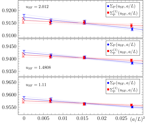
Figure 2: Individual (preliminary) continuum extrapolations of $\Sigma_{\rm P}(u^{\rm SF},a/L)$ and its one-loop improved results $\Sigma_{\rm P}^{(1)}(u^{\rm SF},a/L)$ using all available lattices at fixed SF coupling $u^{\rm SF}\in\{2.012,1.4808,1.110\}$.

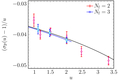
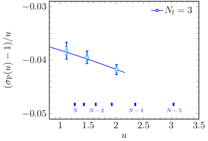
Figure 3: Comparison of step-scaling functions $\sigma_{\rm P}(u^{\rm SF})$ for $N_{\rm f}=2$ (red diamonds) with our preliminary results in the three-flavour theory (blue squares). The solid lines represent the perturbative running using the 2-loop $\tau$-function and 3-loop $\beta$-function in the 2- and 3-flavour theory, respectively.

In the $N_{\rm f}=3$ running coupling project [9, 10], the step-scaling function (SSF) for the RG running of the SF coupling in the high-energy regime, $\sigma_{\rm SF}(u^{\rm SF})$ $(2.012\geq u^{\rm SF}\geq 1.110)$, has been finished. Its determination requires field configurations with non-vanishing boundary conditions on the gauge field [12], while determining renormalization factors, such as ${Z_{\rm P}}$ and thus $\Sigma_{\rm P}$, usually proceeds with vanishing boundary gauge fields. To this end we have started production of $N_{\rm f}=3$ field ensembles for $L/a\in\{6,8,12\}$ and their $2L/a$ counterparts. As for the step-scaling function $\sigma_{\rm SF}$ this is done at 8 values of $u^{\rm SF}$ covering the aforementioned range. The bare parameters for these runs are summarized in Table 1 for the three values $u^{\rm SF}\in\{2.012,1.4808,1.110\}$ at which we already have results on the computationally more expensive $2L/a=24$ lattices. We present preliminary results for the lattice step-scaling $\Sigma_{\rm P}(u,a/L)$ in Figure 2 (blue filled circles), together with its 1-loop improved version (red filled squares), defined by

$$\Sigma_{\rm P}^{(1)}(u,a/L) =\dfrac{\Sigma_{\rm P}(u,a/L)}{1+\delta_{\rm P}(a/L)\,u}\;.$$ (10)

This effectively reduces the leading cutoff effects in the lattice step-scaling function $\Sigma_{\rm P}(u,a/L)$. The coefficients $\delta_{\rm P}(a/L)$ can be inferred from [13]. Although, it is not clear whether the rightmost points for $\Sigma_{\rm P}(u,1/6)$ are still in the region where $(a/L)^{n>2}$ cutoff effects are negligible, cf. [5], for the time being we use all three data points and perform the continuum extrapolation using the ansatz $\Sigma_{\rm P}(u,a/L)=A+B\,(a/L)^{2}$ to determine $A\equiv\sigma_{\rm P}(u)$. We obtain

$u$	$2.012$	$1.4808$	$1.110$
$\sigma_{\rm P}(u)~{}\text{from}~{}\Sigma_{\rm P}$	$0.9173(11)(19)$	$0.9426(8)(17)$	$0.9584(9)(17)$
$\sigma_{\rm P}(u)~{}\text{from}~{}\Sigma_{\rm P}^{(1)}$	$0.9160(11)(8)$	$0.9416(8)(9)$	$0.9576(9)(9)$

where the first error is statistical and the $2^{\text{nd}}$ is the difference to the result of a 2-pt weighted average which neglects the $L/a=6$ data. Our results at fixed $u$ agree well at the one-sigma level. As seen in Figure 2, cutoff effects are reduced in the continuum extrapolation for $\Sigma_{\rm P}^{(1)}$, as to be expected. Accordingly, we can take the values in the third row as our preliminary results for $\sigma_{\rm P}(u^{\rm SF})$ and note that at present the statistical, $\delta_{\rm stat}$, and systematic error, $\delta_{\rm sys}$, are $\lesssim 1\permil$. To get an impression about the quality of these results, we compare them to results obtained for the mass SSF in the two-flavour case. To this end we reproduce Fig.3 of [5] in the left panel of Figure 3 above. We add to the $N_{\rm f}=2$ data (red diamonds) our present results (blue squares) and note that the inner error bar is the purely statistical error, and the outer error bars include the linearly added systematic errors. The latter have been determined as discussed earlier. The two solid lines represent the perturbatively known SSF $\sigma_{\rm P}^{\rm PT}(u)$ to the highest available order in PT, cf. [5], for the $N_{\rm f}=2,3$ flavour cases respectively. The $N_{\rm f}=3$ data falls in line with the PT SSF at small couplings in the SF scheme, best seen in the right panel of the same figure. We furthermore indicate the distribution of the couplings $u^{\rm SF}_{i}=\overline{g}_{\rm SF}^{2}(L_{\rm max}/2^{i})$ as they have been in the $N_{\rm f}=2$ case [3].

The fact that the new data scatters less about the PT behaviour at small couplings compared to $N_{\rm f}=2$, is most likely a result of the intensified and more systematic effort to set up the LCP [9] which has become possible due to algorithmic and computational advancements during the last 10 years. Especially at the switching scale $(u^{\rm SF}=2.012)$, also the total error could be reduced significantly. With 5 additional, uncorrelated continuum data points to be added to this picture soon, $u^{\rm SF}_{i}\in(1.110,2.012)$, we will be in the comfortable position to fit the non-perturbative SSF to much higher accuracy than in the past. However, to give an upper bound on the estimate of the total error of the full $N_{\rm f}=3$ RG running mass factor right now, we can naively assume, using $\Delta[\sigma_{\rm P}]=\delta_{\rm stat}+\delta_{\rm sys}\leq 2\permil$ as discussed above, that

$$\Delta\left[\frac{M}{\kern 1.0pt\overline{\kern-1.0ptm\kern-1.0pt}\kern 1.0pt(\mu_{\rm had})}\right] \simeq\prod_{i}^{N}\Delta[\sigma_{\rm P}(u_{i})]\simeq\sqrt{N}\cdot 2\permil\simeq\begin{cases}0.49\%&\text{for }N=6\quad\text{(as for $N_{\rm f}=2$)}\\ 0.63\%&\text{for }N=10\\ \end{cases}\;.$$ (11)

This means that the total error compared to $N_{\rm f}=2$ will be reduced by at least a factor of 2. Note that we have $N=N_{\rm SF}+N_{\rm GF}$ according to (9). The main assumption entering this upper bound is that we control the error on $\sigma_{\rm P}(u_{i})$ as good in the GF scheme running part at lower energies as we have reported here for the SF scheme running mass part. Needless to say that the naive bound in (11) can be further reduced by increasing the statistics on the lattice SSF to reduce the statictical error even further. But as the systematic error is of the same size as the statistical, it would be better to add another lattice spacing such as $L/a=10$ or $16$ in order to check and further reduce the systematic error in the continuum extrapolation.

4 Summary

We have presented first results towards a computation of the full RG factor for the running mass in three-flavour QCD by the ALPHA collaboration. This is a necessary ingredient to determine renormalization group invariant quark masses from $N_{\rm f}=3$ large-volume ensembles provided by CLS. Systematic errors due to large scale differences are controlled by following a traditional finite-size scaling approach, using the Schrödinger functional as intermediate finite-volume renormalization scheme to non-perturbatively connect low- and high-energy regimes.

A gain in the overall precision is achieved by (a) exploiting very precise results from the ongoing $N_{\rm f}=3$ running coupling project, incorporating a non-perturbative scheme switch at intermediate energies, and (b) via computational advances in algorithms and hardware over the last decade. Both together will allow us to reach an unprecedented precision in the non-perturbative step-scaling function of the mass, provided that equally good results are obtained for the running at lower energies. However, to finally quote an RGI quark mass in physical units, one needs to incorporate the scale-setting procedure which introduces yet another uncertainty and modifies (5) to

$$M_{i} =\frac{M}{\kern 1.0pt\overline{\kern-1.0ptm\kern-1.0pt}\kern 1.0pt(\mu_{\rm had})}\times\lim_{a\to 0}\left[\frac{a\kern 1.0pt\overline{\kern-1.0ptm\kern-1.0pt}\kern 1.0pt_{i}(\mu_{\rm had})}{af_{\rm had}}\right]\times f_{\rm had}\;, \mu_{\rm had} =1/L_{\rm had}\;.$$ (12)

Here $f_{\rm had}$ is any physical quantity that has been used to set the scale on the CLS ensembles.

Together with improvements in the scale-setting procedure w.r.t. the two-flavour case, we can remain optimistic to reach for instance an overall precision less than $1\%$ on $M_{\rm s}$ itself.

References

• [1] M. Lüscher et al., Nucl.Phys. B413 (1994) 481, [hep-lat/9309005].
• [2] ALPHA, M. Della Morte et al., Nucl.Phys. B713 (2005) 378, [hep-lat/0411025].
• [3] ALPHA, P. Fritzsch et al., Nucl.Phys. B865 (2012) 397, [1205.5380].
• [4] ALPHA, S. Capitani et al., Nucl.Phys. B544 (1999) 669, [hep-lat/9810063].
• [5] ALPHA, M. Della Morte et al., Nucl.Phys. B729 (2005) 117, [hep-lat/0507035].
• [6] M. Bruno et al., JHEP 1502 (2015) 043, [1411.3982].
• [7] P. Fritzsch and A. Ramos, JHEP 1310 (2013) 008, [1301.4388].
• [8] A. Ramos and S. Sint, (2015), [1508.05552].
• [9] M. Dalla Brida et al., PoS LATTICE2014 (2014) 291, [1411.7648].
• [10] M. Dalla Brida et al., PoS LATTICE2015 (2015) 248.
• [11] ALPHA, F. Bernardoni et al., Phys.Lett. B730 (2014) 171, [1311.5498].
• [12] M. Lüscher et al., Nucl.Phys. B384 (1992) 168, [hep-lat/9207009].
• [13] ALPHA, S. Sint and P. Weisz, Nucl.Phys. B545 (1999) 529, [hep-lat/9808013].