Non-perturbative tests of continuum HQET through small-volume two-flavour QCD

Abstract

We study the heavy quark mass dependence of selected observables constructed from heavy-light meson correlation functions in small-volume two-flavour lattice QCD after taking the continuum limit. The light quark mass is tuned to zero, whereas the range of available heavy quark masses $m_{\rm h}$ covers a region extending from around the charm to beyond the bottom quark mass scale. This allows entering the asymptotic mass-scaling regime as $1/m_{\rm h}\to 0$ and performing well-controlled extrapolations to the infinite-mass limit. Our results are then compared to predictions obtained in the static limit of continuum Heavy Quark Effective Theory (HQET), in order to verify non-perturbatively that HQET is an effective theory of QCD. While in general we observe a nice agreement at the few-% level, we find it to be less convincing for the small-volume pseudoscalar decay constant when perturbative matching is involved.

1 Introduction

Heavy quark systems, notably B- and ${\rm B}_{\rm s}$-mesons, provide a unique opportunity to perform stringent tests of the Standard Model and probe signals of new physics. To maximize the impact of experiments performed at the Large Hadron Collider, for example, it is imperative to control various aspects of the underlying theory. In particular, strong interaction effects must be understood at the quantitative level, including reliable estimates of systematic uncertainties.

Although in principle lattice QCD in a large physical volume $L^{3}$ allows for ab initio computations of hadronic matrix elements and energy levels, the presence of heavy and light quarks still renders computations very demanding. Current state-of-the-art lattice simulations of QCD with $N_{\rm f}\geq 2$ dynamical quarks usually reach lattice spacings down to $a\sim 0.05\,{\rm fm}$, while satisfying $m_{\pi}L\gtrsim 4$ in order to keep the finite-size effects under control. Due to increasing computer power and algorithmic advances over the last decade, it has become possible to simulate close to the physical pion mass for the figures just given. However, additionally including relativistic b-quarks with their “heavy” physical mass of about $4\,{\rm GeV}$ requires very fine lattice spacings $a\ll 1/m_{\rm h}\sim 0.05\,{\rm fm}$ in order to monitor its discretization effects in the spirit of Symanzik’s local effective theory. Associated with this is the problem of large scale separations, $m_{\rm B}/m_{\pi}={\rm O}(100)$, to be accommodated in a single simulation, which remains out of reach in the near future. Therefore, one still needs to take a detour to an effective description for the heavy quark. Here we focus on the Heavy Quark Effective Theory (HQET) stat:eichten ; Eichten:1989zv ; Georgi:1990um ; Grinstein:1990mj which provides a natural framework to study heavy-light mesons through a systematic expansion in the inverse heavy quark mass, $1/m_{\rm h}$.

A non-perturbative implementation of HQET on the lattice Heitger:2003nj , including the next-to-leading order in the $1/m_{\rm h}$-expansion, has been tested and applied successfully for the quenched case in the past Blossier2010 ; Blossier2010a ; Blossier:2010mk . It requires to solve a set of matching relations between quantities in continuum QCD and lattice HQET in a small physical volume. In two-flavour QCD, the resulting non-perturbative set of HQET parameters Blossier:2012qu was recently used to extract phenomenologically relevant parameters such as the b-quark mass, the B-meson decay constant and hyperfine splittings from large-volume simulations Bernardoni:2013xba ; Bernardoni:2014fva ; Bernardoni:2015nqa . At present there are efforts to extend the matching strategy to include the vector meson channel DellaMorte:2013ega ; Korcyl:2013ega in order to compute $f_{\rm B^{*}}$ and form factors of semi-leptonic ${\rm B}_{({\rm s})}\to\pi\,({\rm K})$ transitions.

In this paper we probe predictions of HQET by studying the asymptotic behaviour $1/m_{\rm h}\to 0$ of continuum-extrapolated lattice QCD observables, computed in a small volume ($L\approx 0.4\,{\rm fm}$) with $N_{\rm f}=2$ dynamical flavours of non-perturbatively ${\rm O}(a)$-improved massless Wilson fermions. Extrapolations to the static limit are performed, which not only gives numerical evidence of the correctness of static order HQET but also allows assessing the size of the $1/m_{\rm h}$-effects. As such, the present study constitutes a non-trivial non-perturbative test of HQET being an effective theory of QCD and extends earlier work in quenched QCD Heitger:2004gb to the physically more realistic situation with dynamical light quarks. In particular, we investigate a considerable set of observables at varied kinematics, which in the spirit of the general non-perturbative matching strategy mentioned above are usually employed to define suitable matching relations. Complementary to perturbative studies Hesse:2012hb ; DellaMorte:2013ega ; Korcyl:2013ega , this yields non-perturbative insights into their heavy quark mass asymptotics and provides criteria for which of them are to be preferred within the matching strategy of Heitger:2003nj , such as impact of mass-dependent cutoff effects in the continuum limit extrapolations, numerical accuracy and magnitude of higher-order corrections in $1/m_{\rm h}$.

In contrast to a non-perturbative matching of (lattice) HQET to continuum QCD, the perturbative approach relies on a perturbative evaluation of matching (resp. conversion) functions, often called Wilson coefficients. To properly recover the static limit in HQET as $m_{\rm h}\to\infty$, also our QCD observables — non-perturbatively evaluated at finite quark mass — still have to be combined with matching functions of this kind. These are only perturbatively known, up to three-loop order in most cases. To disentangle in our tests the genuine non-perturbative properties of the theory encoded in the observables from perturbative effects induced by the conversion functions, we map out their $m_{\rm h}$-dependence towards the static limit for conversion functions of different perturbative orders. This comparison gives a rough idea on the systematic error that is involved, when the matching between HQET and QCD is performed perturbatively. As will be exposed by the example of the pseudoscalar decay constant below, we observe that — with perturbative matching at work — the agreement between the large-mass QCD asymptotics and the HQET prediction may not be as good as expected, even if a three-loop expression for the conversion function is used. We take this as an indication that in an effective theory framework for heavy quarks the matching should be done non-perturbatively, if one wants to have the systematic errors under control. In addition, we consider QCD observables, which have a non-trivial static limit but do not depend on any conversion function. Hence, their $m_{\rm h}\to\infty$ limit is much less affected by systematic uncertainties such that they are among the cleanest observables in our non-perturbative tests of the effective theory approach to heavy-light physics.

Some preliminary results on a smaller subset of observables, data ensembles and statistics have already been reported in DellaMorte:2007qw ; thesis:patrickf .

2 Observables

This paper follows up our previous work Fritzsch:2010aw on the definition of a line of constant physics in $N_{\rm f}=2$ lattice simulations. It allows us to non-perturbatively study the quark mass dependence of relativistic QCD meson observables in a finite box of extent $L_{1}\approx 0.4\,{\rm fm}$ Fritzsch:2012wq . We explore a wide range of quark masses that starts below the charm sector and goes beyond the bottom quark region. This is done in a partially quenched setup, i.e., the light quark mass is set to the approximately vanishing mass of a degenerate sea quark doublet and all other quarks are quenched. We generically refer to the latter as heavy quarks of mass $m_{\rm h}$. Equivalently, we will assign to them the dimensionless mass parameter $z=L_{1}M_{\rm h}$ from now on, where $M_{\rm h}\equiv M$ denotes some fixed value of the renormalization group invariant (RGI) heavy quark mass. In Fritzsch:2010aw we have already shown that in such a small box the lattice spacing can be chosen small enough so that all heavy quarks up to a certain value can be simulated relativistically while keeping cutoff effects in the ${\rm O}(a)$ improved theory well under control. For any unexplained notation, the reader may consult Fritzsch:2010aw ; Heitger:2004gb .

Since our interest lies in relating predictions made by HQET non-perturbatively to the proper counterpart in QCD towards the limit $1/m_{\rm h}\to 0$, we furthermore take into account measurements of HQET observables that have been done in the framework of a general non-perturbative matching strategy of HQET and QCD in the very same volume $L_{1}$, but to a much higher statistical accuracy. Additional details can be found in appendices B and C of reference Blossier:2012qu . Working in a finite (and small) volume, all matrix elements and energies become effective quantities which intrinsically depend on the scale $L_{1}$. For notational brevity we often suppress this dependence in the following.

Our main observables are built from Schrödinger functional (SF) correlation functions Luscher:1992an ; Sint:1993un in a $T\times L^{3}$ volume with $T=L=L_{1}$ fixed and periodic boundary conditions in space. The fermion fields are taken periodic only up to a phase,

$$\psi(x+\hat{k}L) ={\rm e}^{{\rm i}\theta}\psi(x)\;, \overline{\psi}(x+\hat{k}L) =\overline{\psi}(x){\rm e}^{-{\rm i}\theta}\;, k =1,2,3\;,$$ (1)

where we use $\theta\in\{0,0.5,1\}$. In correlation functions, this periodicity angle $\theta$ amounts to a projection onto quark and antiquark momenta with components $\pm\theta/L$. In time direction, Dirichlet boundary conditions are imposed at $x_{0}=0,\,T$ where source quark and antiquark fields are separately projected onto vanishing spatial momentum. We are interested in the pseudoscalar (PS) and vector (V) channel using finite-volume heavy-light QCD currents. They are given by the time component of the axial vector and spatial components of the vector current, respectively:

$$A_{0}(x_{0}) =\overline{\psi}_{\rm l}(x_{0})\gamma_{0}\gamma_{5}\psi_{\rm h}(x_{0})\;, V_{k}(x_{0}) =\overline{\psi}_{\rm l}(x_{0})\gamma_{k}\psi_{\rm h}(x_{0})\;, 0 <x_{0}<T\;.$$ (2)

To be more precise, we use their ${\rm O}$ improved DellaMorte:2005se ; Sint:1997jx and non-perturbatively renormalized DellaMorte:2008xb lattice versions. Furthermore, we need the pseudoscalar heavy-light current

$$P(x_{0}) =\overline{\psi}_{\rm l}(x_{0})\gamma_{5}\psi_{\rm h}(x_{0})\;, 0 <x_{0}<T\;,$$ (3)

the renormalization factor of which, $Z_{\rm P}(\mu,g_{0}^{2})$, has been determined non-perturbatively in the SF scheme at scale $\mu=1/L_{1}$ during the production runs reported in Blossier:2012qu . Since they have not been quoted in that reference we list them together with further details in table 4.

2.1 Definitions

How to non-perturbatively set up a line of constant physics in the envisaged small volume $L_{1}\approx 0.4\,{\rm fm}$ has already been reported in Fritzsch:2010aw . In that volume we have four different ensembles with non-perturbatively ${\rm O}$ improved dynamical Wilson fermions made of a doublet of massless quarks. The range of lattice spacings used is $0.01\,{\rm fm}\lesssim a\lesssim 0.02\,{\rm fm}$. This ensures feasible continuum limit extrapolations of the QCD observables to be introduced below, which depend on the dimensionless RGI heavy quark mass fixed to

$$z \equiv L_{1}M_{\rm h}\in\{2,2.7,3,3.3,4,6,7,9,11,13,15,18,21\}\;.$$ (4)

In contrast to our previous work, we added four additional $z$-values at the lower end to also cover the charm quark region. Details about the latter, which were needed to perform the additional measurements, are listed in table 4. In the computation of HQET observables we can naturally rely on larger lattice spacings ($0.025\,{\rm fm}\lesssim a\lesssim 0.067\,{\rm fm}$). We use the “HQET[$L_{1}$]” lattices with $T=L=L_{1}$ as specified in table C.1 and C.2 of ref. Blossier:2012qu . For completeness we list some additional details in table 5 that were not published there.

The HQET observables themselves are computed using two different static actions, referred to as ${\rm HYP1}$ and ${\rm HYP2}$ DellaMorte:2005yc , in order to have an improved noise-to-signal behaviour compared to the original Eichten-Hill action. For the present purpose of testing HQET we want to express all observables in terms of matrix elements computed in a finite volume. The interested reader can find the corresponding notation in terms of the traditional SF correlation functions in appendix A and reference Heitger:2004gb . In passing we just note that only states, which are eigenstates of spatial momentum with eigenvalue zero, enter them.

2.2 Effective masses

The small-volume effective pseudoscalar and vector meson mass in terms of Hilbert space matrix elements read, adopting an operator notation for the quark bilinear composite fields,

$$\Gamma_{\rm PS}(x_{0}) =-\widetilde{{\partial_{0}}}\ln\big{[}\langle\Omega(L)|{\,\mathbb{A}_{0}}|{\rm B}(L)\rangle\big{]}\;,$$ (5a)

$$\Gamma_{\rm V}(x_{0}) =-\widetilde{{\partial_{0}}}\ln\big{[}\langle\Omega(L)|{\,\mathbb{V}_{k}}|{\rm B}^{*}(L)\rangle\big{]}\;,$$ (5b)

$$\Gamma_{\rm P}(x_{0}) =-\widetilde{{\partial_{0}}}\ln\big{[}\langle\Omega(L)|{\,\mathbb{P}}\,|{\rm B}(L)\rangle\big{]}\;,$$ (5c)

where $|\Omega(L)\rangle\equiv{\rm e}^{-x_{0}{\,\mathbb{H}}}|\varphi_{0}(L)\rangle$ denotes the vacuum state given in terms of the Hamiltonian ${\,\mathbb{H}}$ and the SF intrinsic vacuum boundary state $|\varphi_{0}(L)\rangle$ at $x_{0}=0$. Having in mind a variation of the heavy quark mass for our non-perturbative tests later on, we denote a general heavy-light pseudoscalar state by $|{\rm B}(L)\rangle\equiv{\rm e}^{-x_{0}{\,\mathbb{H}}}|\varphi_{{\rm B}}(L)\rangle$ and a heavy-light vector state by $|{\rm B}^{*}(L)\rangle\equiv{\rm e}^{-x_{0}{\,\mathbb{H}}}|\varphi_{{\rm B}^{*}}(L)\rangle$. Both are again given through the time evolution operator and the well-defined boundary states $|\varphi_{\rm X}\rangle$ with quantum numbers in the respective channel, ${\rm X}={\rm B},{\rm B}^{*}$. Since all states naturally depend on the finite volume (or box) size $L$ and are also considered as functions of the RGI heavy quark mass $M$ (or $z$), we drop these dependencies for the moment to ease notation, as we do so for their additional dependence on the SF-specific periodicity angle $\theta$ of the fermion fields. Here and from now on, we fix $x_{0}=T/2\equiv L/2$ in the correlation functions employed to construct the observables above and those to be introduced in the subsections below. It is then worth to emphasize that the time evolution operator ${\rm e}^{-T{\,\mathbb{H}}/2}$ suppresses high-energy states exponentially such that $|\Omega(L)\rangle$ and $|{\rm B}(L)\rangle$, upon expanding them in terms of eigenstates of ${\,\mathbb{H}}$, are dominated by contributions from states with energies of at most $\Delta E={\rm O}(1/L)$ above the ground state. Therefore, as HQET is expected to apply to correlation functions at large Euclidean time separations, it particularly describes their large-mass behaviour at large $x_{0}\geq{\rm O}(1/m_{\rm h})$ in the present SF setup, too.

Whereas physical masses must be computed in large-volume simulations, the definition of our observables is such that they agree with the physical ones in the large-volume limit $L\to\infty$.

2.3 Decay constants and ratios

Furthermore and analogously, we define the following QCD observables, suppressing again their dependence on $M$, $L$ and $\theta$:

$$Y_{\rm PS} \equiv+\left[\dfrac{\langle\Omega|{\,\mathbb{A}_{0}}|{\rm B}\rangle}{|\!|{|\Omega\rangle}|\!|\cdot|\!|{|\rm B\rangle}|\!|}\right]_{\rm R}\;, Y_{\rm V} \equiv-\left[\dfrac{\langle\Omega|{\,\mathbb{V}_{k}}|{\rm B}^{*}\rangle}{|\!|{|\Omega\rangle}|\!|\cdot|\!|{|\rm B^{*}\rangle}|\!|}\right]_{\rm R}\;,$$ (6)

$$R_{\rm PS/P} \equiv-\left[\dfrac{\langle\Omega|{\,\mathbb{A}_{0}}|{\rm B}\rangle}{\langle\Omega|{\,\mathbb{P}}\,|{\rm B}\rangle}\right]_{\rm R}\;, R_{\rm PS/V} \equiv-\left[\dfrac{\langle\Omega|{\,\mathbb{A}_{0}}|{\rm B}\rangle}{\langle\Omega|{\,\mathbb{V}_{k}}|{\rm B}^{*}\rangle}\right]_{\rm R}\;,$$ (7)

$$Y_{\rm PS/V} \equiv\dfrac{Y_{\rm PS}}{Y_{\rm V}}\;, R_{\rm spin} \equiv\dfrac{3}{4}\ln\dfrac{\langle{\rm B}|{\rm B}\rangle}{\langle{\rm B}^{*}|{\rm B}^{*}\rangle}\;,$$ (8)

where $Y_{\rm PS}$ and $Y_{\rm V}$ are the finite-volume heavy-light pseudoscalar and vector decay constant, respectively. As $L\to\infty$, they become proportional to the physical heavy-light pseudoscalar and vector meson decay constants. Accordingly, $Y_{\rm PS/V}$ is the ratio of the two, which in large volume becomes proportional to $f_{\rm B}/f_{\rm B^{*}}$, if the heavy quark is set to the b-quark. The ratio $R_{\rm spin}$ is proportional to the spin splitting between the pseudoscalar and vector channel and, as predicted by HQET, has to vanish in the static limit owing to the heavy-quark spin symmetry. These observables also involve boundary-to-boundary SF correlation functions, see appendix A, which properly cancel the multiplicative renormalization factors of the boundary quark fields.

All quantities involving $[\bullet]_{\rm R}$ are understood to be renormalized non-perturbatively, while for others such factors either drop out or are not needed at all, such that alltogether they thus are finite and possess a well-defined continuum limit.

2.4 Quantities with different kinematics

The SF is especially useful, if one wants to probe physics with different kinematics. Here we do so by changing the fermionic phase angle $\theta$ as mentioned earlier. Whereas in the last section all observables were meant to be evaluated at the same values, i.e., $\theta_{0}\in\{0,0.5,1\}$, we now turn our attention to quantities that are made of two matrix elements of heavy-light composite fields referring to fermionic periodicity phases different from eachother. With the same notational conventions as before they read

$$R_{f}(\theta_{1},\theta_{2}) =\frac{\langle{\rm B}|{\rm B}\rangle_{\theta_{1}}}{\langle{\rm B}|{\rm B}\rangle_{\theta_{2}}}\;, R_{\rm PS/PS}(\theta_{1},\theta_{2}) =\frac{\langle\Omega|{\,\mathbb{A}_{0}}|{\rm B}\rangle_{\theta_{1}}}{\langle\Omega|{\,\mathbb{A}_{0}}|{\rm B}\rangle_{\theta_{2}}}\;,$$ (9a)

$$R_{k}(\theta_{1},\theta_{2}) =\frac{\langle{\rm B}^{*}|{\rm B}^{*}\rangle_{\theta_{1}}}{\langle{\rm B}^{*}|{\rm B}^{*}\rangle_{\theta_{2}}}\;, R_{\rm V/V}(\theta_{1},\theta_{2}) =\frac{\langle\Omega|{\,\mathbb{V}_{k}}|{\rm B}^{*}\rangle_{\theta_{1}}}{\langle\Omega|{\,\mathbb{V}_{k}}|{\rm B}^{*}\rangle_{\theta_{2}}}\;,$$ (9b)

$$R_{1}(\theta_{1},\theta_{2}) =\frac{1}{4}\ln\left[R_{f}(\theta_{1},\theta_{2})R_{k}(\theta_{1},\theta_{2})^{3}\right]\;, R_{\rm P/P}(\theta_{1},\theta_{2}) =\frac{\langle\Omega|{\,\mathbb{P}}\,|{\rm B}\rangle_{\theta_{1}}}{\langle\Omega|{\,\mathbb{P}}\,|{\rm B}\rangle_{\theta_{2}}}\;,$$ (9c)

$$Y_{\rm PS/PS}(\theta_{1},\theta_{2}) =\frac{Y_{\rm PS}(\theta_{1})}{Y_{\rm PS}(\theta_{2})}\;, Y_{\rm V/V}(\theta_{1},\theta_{2}) =\frac{Y_{\rm V}(\theta_{1})}{Y_{\rm V}(\theta_{2})}\;,$$ (9d)

where in our actual calculations we consider the following pairs of phase angles: $(\theta_{1},\theta_{2})\in\{(0,0.5),(0.5,1),(0,1)\}$.

It is important to note that all multiplicative renormalization and improvement factors cancel in these ratios. In this respect and because one expects cancellations of cutoff effects at every fixed value of $z$, these QCD observables (as well as their counterparts in HQET) may be seen as “gold plated” observables for the purpose of testing the asymptotic behaviour of heavy-light physics as $z\to\infty$ for different kinematical setups.

2.5 Observables in HQET

After the continuum limit of the previously defined QCD observables has been taken, we aim for an extrapolation to the static limit, $1/z\to 0$, in order to compare their asymptotic behaviour to the one predicted by HQET in the continuum. According to the systematic heavy quark expansion, all quantities approach a well-defined value in that limit. Classically, the leading asymptotic behaviour of our effective masses (5), for instance, is linear in the heavy quark mass $z$, but it receives logarithmic modifications on the quantum level owing to the scale dependent renormalization of the effective theory to compare with, viz.

$$L\Gamma(L,M)\; \raisebox{-0.43057pt}{$\stackrel{{\scriptstyle\small{z\to\infty}}}{{\sim}}$}\;C_{\rm mass}(z)\cdot z\cdot\Big{[}1+{\rm O}\big{(}z^{-1}\big{)}\Big{]}\;,$$ (10)

where $C_{\rm mass}(z)$ denotes the conversion function that relates the heavy quark’s pole mass to the RGI heavy quark mass $M=z/L_{1}$.

A generic conversion function $C_{\rm X}(z)$ carries all the logarithmic dependence of a given quantity $\rm X$ to some order in perturbation theory such that only power corrections in $1/z$ remain in the effective theory. For more details, we refer to appendix B and appendix B of Heitger:2004gb . To avoid a remnant renormalization scheme dependence in the (static) effective theory, we favour to fully express the asymptotic behaviour in terms of renormalization group invariants (RGIs). For the quantities of section 2.3, i.e., $\rm X\in\{{\rm PS},{\rm V},{\rm PS/P},{\rm PS/V},{\rm spin}\}$, this means

$$Y_{\rm PS}(L,M)\; \raisebox{-0.43057pt}{$\stackrel{{\scriptstyle\small{z\to\infty}}}{{\sim}}$}\;C_{\rm PS}(z)\cdot X_{\rm RGI}(L)\cdot\Big{[}1+{\rm O}\big{(}z^{-1}\big{)}\Big{]}\;,$$ (11)

$$Y_{\rm V}(L,M)\; \raisebox{-0.43057pt}{$\stackrel{{\scriptstyle\small{z\to\infty}}}{{\sim}}$}\;C_{\rm V}(z)\cdot X_{\rm RGI}(L)\cdot\Big{[}1+{\rm O}\big{(}z^{-1}\big{)}\Big{]}\;,$$ (12)

$$R_{\rm PS/P}(L,M)\; \raisebox{-0.43057pt}{$\stackrel{{\scriptstyle\small{z\to\infty}}}{{\sim}}$}\;C_{\rm PS/P}(z)\cdot 1\cdot\Big{[}1+{\rm O}\big{(}z^{-1}\big{)}\Big{]}\;,$$ (13)

$$R_{\rm PS/V}(L,M)\; \raisebox{-0.43057pt}{$\stackrel{{\scriptstyle\small{z\to\infty}}}{{\sim}}$}\;C_{{\rm PS}/{\rm V}}(z)\cdot 1\cdot\Big{[}1+{\rm O}\big{(}z^{-1}\big{)}\Big{]}\;,$$ (14)

$$Y_{\rm PS/V}(L,M)\; \raisebox{-0.43057pt}{$\stackrel{{\scriptstyle\small{z\to\infty}}}{{\sim}}$}\;C_{{\rm PS}/{\rm V}}(z)\cdot 1\cdot\Big{[}1+{\rm O}\big{(}z^{-1}\big{)}\Big{]}\;,$$ (15)

$$R_{\rm spin}(L,M)\; \raisebox{-0.43057pt}{$\stackrel{{\scriptstyle\small{z\to\infty}}}{{\sim}}$}\;C_{\rm spin}(z)\cdot\frac{X_{\rm RGI}^{\rm spin}(L)}{z}\cdot\Big{[}1+{\rm O}\big{(}z^{-1}\big{)}\Big{]}\;.$$ (16)

The ratios $R_{\rm PS/P}$, $R_{\rm PS/V}$ and $Y_{\rm PS/V}$, along with the associated $C_{\rm X}$, approach $1$ in the static limit of HQET, whereas the effective decay constants $Y_{\rm PS}$ and $Y_{\rm V}$ both approach the finite-volume RGI static-light decay constant $X_{\rm RGI}(L)$ in this limit, as a consequence of the heavy-quark spin symmetry. In the two-flavour theory at hand DellaMorte:2006sv , the renormalization scale was implicitly fixed by a value for the renormalized SF coupling of $\bar{g}^{2}(\mu)|_{\mu=L_{\rm max}^{-1}}\equiv 4.61$. However, since for the purpose of this study we are working at a slightly different physical volume $L_{1}\,\lesssim\,L_{\rm max}$, the universal part $Z^{\rm stat}_{\rm A,RGI}/Z^{\rm stat}_{\rm A}(\mu)$ of the total renormalization factor, which relates a matrix element of the static axial current renormalized at a scale $\mu$, $X_{\rm R}(\mu)$, to the RGI one, had to be re-evaluated. The outcome for $\mu=L_{1}^{-1}$ based on the data of DellaMorte:2006sv is

$$X_{\rm RGI} =\frac{Z^{\rm stat}_{\rm A,RGI}}{Z^{\rm stat}_{\rm A}(\mu)}\cdot X_{\rm R}(\mu)\;, \left.\frac{Z^{\rm stat}_{\rm A,RGI}}{Z^{\rm stat}_{\rm A}(\mu)}\right|_{\mu=L_{1}^{-1}}\!\!\! =0.875(7)\;, \left.\bar{g}^{2}(\mu)\right|_{\mu=L_{1}^{-1}} \equiv 4.484\;,$$ (17)

which allows us to directly compute the (renormalization scale and scheme independent) quantity $X_{\rm RGI}$ instead of the renormalized (and thus scale dependent) static-light decay constant $X_{\rm R}(\mu)$ in finite volume. Some additional technical details on $X_{\rm RGI}$ and its error budget are postponed to appendix C.

By contrast, the RGI matrix element of the spin splitting operator, $X_{\rm RGI}^{\rm spin}$, is not known, because the corresponding RG running is not available for the dynamical flavour theory. Note that in principle it would be possible to extract it from our QCD data according to the given asymptotic behaviour, (16), but with the only perturbatively known conversion function $C_{\rm spin}$ we do not expect the result to be particularly meaningful.

Our most stringent tests of HQET will finally arise from the QCD observables defined in section 2.4. In these quantities, the conversion functions cancel such that no logarithmic corrections are left to all orders in perturbation theory and non-perturbatively. Hence, all uncertainties from the matching between QCD and HQET are absent and one just faces the genuine power corrections in $1/z$ of the effective theory. This makes the comparison of continuum QCD in the limit $1/z\to 0$ and continuum HQET at static order entirely non-perturbative and very well controllable, without encountering any systematic errors induced by the perturbatively evaluated $C_{\rm X}$. Exploiting again the heavy-quark symmetry, the HQET counterparts of these QCD observables in the static limit are:

$$R_{f}^{\rm stat}(\theta_{1},\theta_{2}) =\exp\left[\lim_{1/z\to 0}R_{1}(z,\theta_{1},\theta_{2})\right]=\lim_{1/z\to 0}R_{\rm i}(z,\theta_{1},\theta_{2})\;, \text{for }{\rm i} =f,k\;,$$ (18a)

$$R_{\rm PS}^{\rm stat}(\theta_{1},\theta_{2}) =\lim_{1/z\to 0}R_{\rm i/i}(z,\theta_{1},\theta_{2})\;, \text{for }{\rm i} ={\rm PS},{\rm V},{\rm P}\;,$$ (18b)

$$R_{X}^{\rm stat}(\theta_{1},\theta_{2}) =\lim_{1/z\to 0}Y_{\rm i/i}(z,\theta_{1},\theta_{2})\;, \text{for }{\rm i} ={\rm PS},{\rm V}\;.$$ (18c)

3 Results

In the following subsections we first discuss exemplary continuum extrapolations for some of our test observables before we turn our attention to the main results, i.e., their extrapolations as $1/z\to 0$ to the static limit of HQET. Additional details about our continuum extrapolations can be found in appendix C.

3.1 Representative continuum extrapolations

For the quantities of subsections 2.2 – 2.4, which as properly renormalized QCD observables are now generically denoted by $\Omega^{\rm QCD}=\Omega^{\rm QCD}(L,M,a)$, we perform extrapolations to the continuum limit (CL) using a global fit ansatz in order to have better control over mass-dependent lattice artefacts. Due to the latter, we exclude some points at coarsest lattice spacings from these global QCD continuum extrapolations.

In general we aim at taking the continuum limit of a QCD observable according to the global fit ansatz

$$\Omega^{\rm QCD}(L,z,a) =\Omega^{\rm QCD}(L,z)\left[1+(a/L)^{2}\cdot\left\{\rho_{0}+\rho_{1}z+\rho_{2}z^{2}\right\}\right]\;,$$ (19)

which accounts for terms proportional $a/L\times aM$ and $(aM)^{2}$. From earlier studies Kurth:2001yr ; Heitger:2004gb it is known that an exclusion limit of $aM>0.7$ has to be imposed on the data entering in the extrapolating fits, in order to avoid contaminations which are potentially dangerous for a reliable continuum limit.

To assure stability in our CL results, different fit ansaetze have also been studied (e.g., allowing for a cubic term in $a/L$ with mass-dependent coefficient or omitting some of the lightest masses, say $z\leq 4$); these lead to consistent results. As the general scaling behaviour towards the continuum limit looks rather similar among the different observables, we only show two representative examples here. In the left panel of figure 1 we present the result for the effective pseudoscalar decay constant at $\theta_{0}=0.5$ and in the right the outcome for a ratio of the same quantity evaluated at different kinematical parameters, namely at $(\theta_{1},\theta_{2})=(0.5,1)$.

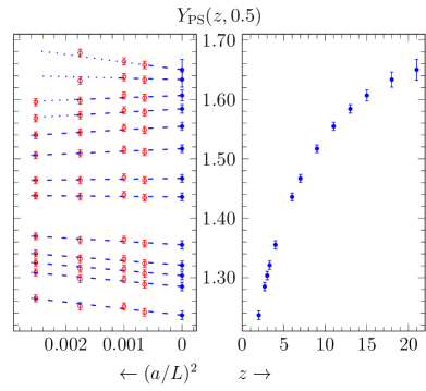
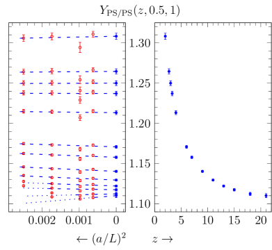
Figure 1: Continuum extrapolation and resulting continuum $z$-dependence of $Y_{\rm PS}(\theta_{0},z)$ (left) and $Y_{\rm PS/PS}(\theta_{1},\theta_{2},z)$ (right). Dashed lines of the continuum extrapolation cover data points that enter the global fit, while the dotted part extends to all points. The data points used and shown have been tree-level improved in advance, cf. appendix C.

As yet we have not taken into account the error stemming from the tuning of the heavy quark mass (4) at finite lattice spacing. The uncertainty of the continuum heavy quark mass $M=z/L_{1}$ is $\Delta M/M=\Delta z/z=1.01\%$ Fritzsch:2010aw . We add its error

$$\Delta_{M}\Omega^{\rm QCD}(L,M,0) =\frac{\partial\Omega^{\rm QCD}(L,M,0)}{\partial M}\,\Delta M$$ (20)

quadratically, before performing any extrapolations to the static limit as they are presented in the following subsections. The derivative is estimated numerically from the data at hand. Its contribution to the total error budget is actually negligible, as can be inferred from the continuum mass dependence displayed in figure 1, for instance. In appendix C we list a representative selection of results at finite lattice spacing and its continuum limit.

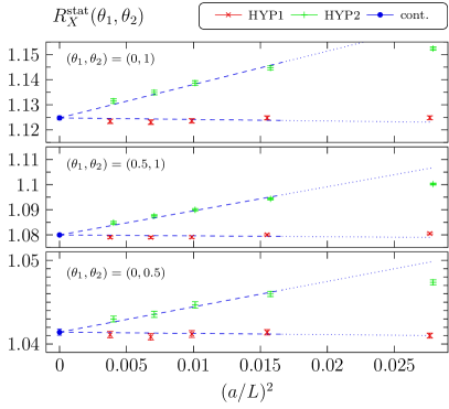
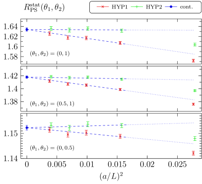
Figure 2: Continuum extrapolations of two representative static observables at different kinematical parameters.

In some cases, continuum extrapolations of associated observables in HQET have also to be performed. Taking the continuum limit of observables in the static theory is much more straightforward, because there is obsviously no dependence on $z$ and thus no mass-dependent cutoff effect that needs to be controlled in addition. However, they depend on the two static actions employed here (HYP$i$, $i=1,2$), and hence this suggests to adopt a joint continuum extrapolation of a given HQET observable according to

$$\Omega^{\rm HQET}_{i}(L,a) =\Omega^{\rm HQET}(L)\left[1+(a/L)^{2}\cdot A_{i}\right]\;.$$ (21)

As two explicit examples we show in figure 2 the continuum extrapolation of $R_{X}^{\rm stat}(\theta_{1},\theta_{2})$ and $R_{\rm PS}^{\rm stat}(\theta_{1},\theta_{2})$. The numerical results are listed in table 2 and 3, respectively.

Before turning our attention to the main results, we want to add some general remarks on their presentation and the analysis underlying them.

3.2 Results including perturbative conversion functions

As emphasized before, for certain (continuum-extrapolated) observables $\Omega^{\rm QCD}(L,M,0)\equiv\Omega^{\rm QCD}(L,z)$ we need to take into account logarithmic corrections when comparing HQET with QCD in the heavy quark mass limit. Hence, we divide by the corresponding conversion function $C_{\Omega}(M/\Lambda_{\overline{{\rm MS}}})$ and, in a few cases where convenient, cancel the leading mass dependence by an appropriate multiplication with some power $\ell$ of $z$, such as $\ell=-1$ in the case of $\Omega=L\Gamma$, for instance. An exactly — or even non-perturbatively — known conversion function by definition removes all logarithmic contributions, while the remainder can then be assumed to be organized as a “power series” in $1/z$, resembling continuum HQET in the asymptotic regime of large $z$. We thus perform extrapolations to the static limit of HQET of quantities with perturbative conversion functions according to the fit ansatz

$$\left[z^{\ell}\cdot\Omega^{\rm QCD}(L,M,0)\big{/}C_{\Omega}(M/\Lambda_{\overline{{\rm MS}}})\right] =\Omega^{[0]}+\Omega^{[1]}z^{-1}+\Omega^{[2]}z^{-2}\;,\quad z^{-1}\lesssim 0.26\;,$$ (22)

where $\Omega^{[0]}$ represents the static limit of the observable in question as extracted through this fit from the relativistic QCD data. (The choice $1/z\lesssim 0.26$ is motivated below.) In practice, we must rely on a perturbative evaluation of the conversion functions up to limited order that have uncertainties decreasing only logarithmically (see, e.g., ref. Sommer:2010ic ). Since those have to be combined with our non-perturbative lattice data, we generically cannot disentangle logarithmic and power-like contributions exactly up to some definite value of $1/z$. A safe statement that can be made, however, is that one asymptotically expects eq. (22) to yield a good description of the data in the sense that the l.h.s. of (22) approaches $\Omega^{[0]}$ in the limit $z\to\infty$. To what extent a quantity $\Omega^{[0]}$ agrees with its HQET counterpart is subject of the discussion below.

To represent our data, we employed several unconstrained (and weighted) polynomial fits in $1/z$ along (22) by varying the range of points that enter the fit with the degree of the polynomial. Even though the full data set — down to masses of $\sim 70\%$ of the charm quark mass — is well described by a quadratic interpolation within our statistical accuracy, it is not surprising that this variation, depending on the observable under consideration, has a visible effect on the result of the static extrapolation. More precisely, we observe the clear general trend (motivating the $z$-range choice in (22)) that a fit of degree $n$ should include data in the interval $[0,n\cdot\Delta z^{-1}]$, with $\Delta z^{-1}\approx 0.13$, in order to keep the static limit unchanged (within errors) and thereby independent of the employed polynomial fit ansatz. This statement holds separately true for the data incorporating $C_{\Omega}$ evaluated at two- or three-loop order in perturbation theory. However, as will become evident in the sequel, the dominantly significant, systematic effect on the static extrapolation results originates from the only perturbative knowledge of the conversion functions that are required to relate QCD observables at finite $z$ to their HQET counterparts, before the static limit is taken.

Asymptotic behaviour of effective meson masses

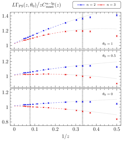
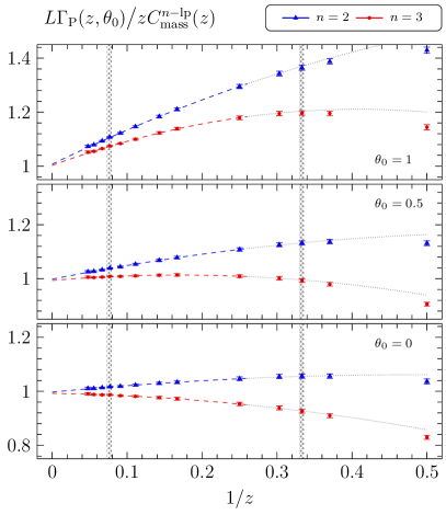
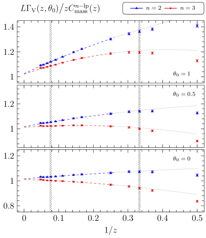
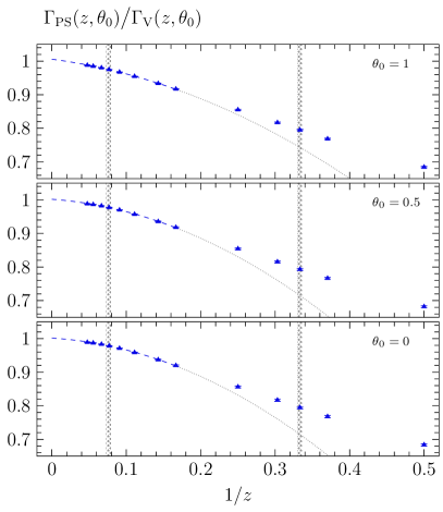
Figure 3: Subleading asymptotic behaviour of effective meson masses at different kinematical parameters using two- and three-loop conversion functions. In comparison, the lower right panel shows the asymptotic behaviour of the ratio of effective pseudoscalar and vector meson masses. In this ratio, QCD-HQET conversion functions and the leading power in $z$ cancel.

First, we study the large quark mass behaviour of the effective meson masses (5) according to its leading asymptotics in this regime that is given by eq. (10). The raw data and the continuum-extrapolated values for representative $\theta$-values are collected in tables 6 and 7 of appendix C. Following eq. (22), we combine the effective meson masses with their associated conversion function $C_{\rm mass}$ and remove the leading heavy quark mass dependence. The remaining finite piece of $\left[L\Gamma_{\rm X}(L,M,0)\big{/}\big{(}zC_{\rm mass}(M/\Lambda_{\overline{{\rm MS}}})\big{)}\right]$ then should approach $1$ in the static (i.e., $1/z\to 0$) limit for all ${\rm X}={\rm PS},{\rm V},{\rm P}$.

Figure 3 confirms this expectation, where for each individual observable and $\theta_{0}\in\{0,0.5,1\}$ we depict the remaining (i.e., subleading) asymptotic behaviour of our continuum data points for the effective meson masses using $C_{\rm mass}$ evaluated at two- and three-loop order, cf. eq. (44). For ease of presentation, only the statistical errors of $L\Gamma_{\rm X}(z,\theta_{0})$ are included in the figures. With the fit ansatz (22) and all errors taken into account, the results in the static limit, $\Omega^{[0]}_{\rm X}$, agree for all ${\rm X}={\rm PS},{\rm V},{\rm P}$ with $1$ within errors indeed. In order to better judge the validity range of the asymptotic $1/z$-expansion reflected by the extrapolating fits to the static limit — as well as the size of possible particular systematic effects at the physical scale of the b- and c-quark — here and in subsequent figures we add vertical error bands corresponding to $z_{\rm b}=L_{1}M_{\rm b}\approx 13.25$ Bernardoni:2013xba and $z_{\rm c}=L_{1}M_{\rm c}\approx 3.04$ Heitger:2013oaa .

Another non-trivial test consists in studying ratios of masses, in which the leading asymptotics drops out completely. Such a case is displayed in the bottom-right panel of figure 3. This is a first explicit example with the heavy-quark spin symmetry at work, according to which HQET predicts $\lim_{1/z\to 0}[\Gamma_{\rm PS}/\Gamma_{\rm V}]=1$. The deviation from one at the b-quark scale ($z=z_{\rm b}$), dominated by the spin-splitting term, is about $2\%$. With increasing $1/z$, higher-order terms appear to become relevant and contribute with opposite signs, leading to a deviation of about $20\%$ at the charm quark mass scale. At least for $\Gamma_{\rm PS}/\Gamma_{\rm V}$, this supports the general expectation that HQET does not provide an all too good description for charm physics any more.

Asymptotic behaviour of ratios of heavy-light currents

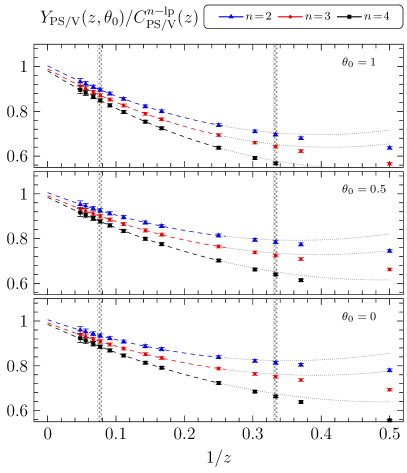
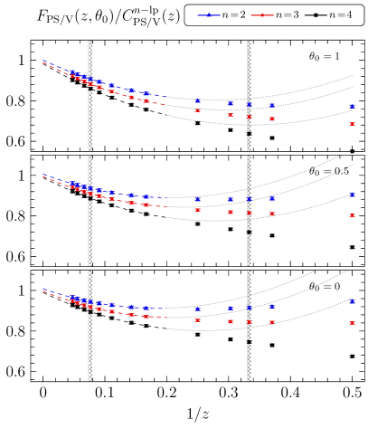
Figure 4: Asymptotic behaviour of ratios of effective decay constants at different kinematical parameters involving two-, three- and four-loop conversion functions.

Owing to the definitions in subsections 2.2 and 2.3, the finite-volume continuum QCD observable $Y_{\rm PS/V}=Y_{\rm PS}/Y_{\rm V}$ approaches in the large-volume limit a combination of ratios of pseudoscalar to vector heavy-light meson decay constants and masses, which becomes of phenomenological relevance at the b-quark mass scale:

$$\lim_{L\to\infty}Y_{\rm PS/V}(z,\theta_{0})\big{|}^{z=z_{\rm b}}_{\theta_{0}=0} =\frac{f_{\rm B}}{f_{\rm B^{*}}}\sqrt{\frac{m_{\rm B}}{m_{\rm B^{*}}}}\;.$$ (23)

Thus it is interesting to also inspect the $1/z$-dependence of $Y_{\rm PS/V}$. As before, after extrapolating to the continuum limit and accounting for the proper full (logarithmic) mass dependence via attaching the function $C_{\rm PS/V}(z)$ to two-, three- and even four-loop accuracy, cf. eq. (43), we obtain $Y_{\rm PS/V}(z,\theta_{0})$ and the corresponding extrapolations to the static limit of HQET reproduced in the left panel of figure 4. Again, we find that for every $\theta_{0}$ the static HQET prediction ($=1$) is reached within errors, with an almost linear approach as $1/z\to 0$ for $z>10$; its slope grows with the flavour-twisted momentum $\theta_{0}$.

As discussed in appendix B, the conversion formula for the ratio of decay constants ${f_{\rm B}}/{f_{\rm B^{*}}}$, $C_{{\rm PS}/{\rm V}}$, is even known to four-loop accuracy Bekavac2010 , because in the entering difference of anomalous dimensions the unknown four-loop anomalous dimensions of the currents themselves drop out. It was already noted in Bekavac2010 ; Sommer:2010ic (and is also reflected in the middle-right panel of figure 10 in appendix B) that the perturbative expansion of $C_{{\rm PS}/{\rm V}}$ exhibits a bad behaviour, since the perturbative coefficients grow further with the loop order such that the concept of asymptotic convergence of the perturbative series appears to be meaningful only for rather small couplings or masses far above the mass of the b-quark. At the scale of the b-quark mass, for instance, every known perturbative order approximately contributes by an equal amount. The worrying behaviour of perturbation theory for $C_{{\rm PS}/{\rm V}}$ may also be read off from the data points in figure 4, where in fact no signs of an asymptotic convergence with the loop order in $C_{{\rm PS}/{\rm V}}$ from about the b-quark mass scale on of any of the curves through the points can be stated. This is even more so for

$$F_{\rm PS/V}(z,\theta_{0}) \equiv Y_{\rm PS/V}(z,\theta_{0})\left({\frac{\Gamma_{\rm PS}(z,\theta_{0})}{\Gamma_{\rm V}(z,\theta_{0})}}\right)^{-1/2}\;,$$ (24)

in the right panel of figure 4, as a direct effective finite-volume estimates of ${f_{\rm B}}/{f_{\rm B^{*}}}$ involving $C_{{\rm PS}/{\rm V}}$, too, where $\Gamma_{\rm PS}/\Gamma_{\rm V}$ cancels the ratio of meson masses in $Y_{\rm PS/V}$. The growing deviations of the data points from the polynomial fits in $1/z$ towards the charm quark scale for this quantity are inherited from the corresponding behaviour of the higher-order terms in $\Gamma_{\rm PS}/\Gamma_{\rm V}$ (see previous paragraph).

Asymptotic behaviour of effective decay constants

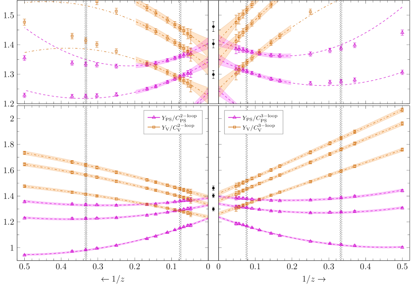
Figure 5: Comparison of the static extrapolations of $Y_{\rm PS}(\theta_{0},z)$ and $Y_{\rm V}(\theta_{0},z)$ to the non-perturbative HQET results in the continuum (indicated as the data points in the middle bewteen the panels). In the left panels we use conversion functions $C_{\rm X}$, $\rm X={\rm PS},{\rm V}$, evaluated at two-loop, while in the right panels they are evaluated at three-loop order of perturbation theory. Additionally, the lower panels show (weighted) quadratic fits to all data points, while the upper panels only include data points in the expected applicability domain of HQET ($1/z<0.2$). A linear extrapolation over the further restricted range $1/z\lesssim 0.13$ would lead to compatible results.

	static limit in QCD		static HQET	static limit in QCD
	for $1/z<0.2$			for $1/z\leq 0.5$
$\theta_{0}$	$Y_{\rm PS}^{[0]}$	$Y_{\rm V}^{[0]}$	$X_{\rm RGI}$	$Y_{\rm PS}^{[0]}$	$Y_{\rm V}^{[0]}$
$0.0$	$1.413(20)$	$1.413(33)$	$1.461(17)$	$1.3978(57)$	$1.4206(50)$
$0.5$	$1.348(18)$	$1.350(32)$	$1.403(11)$	$1.3427(48)$	$1.3642(45)$
$1.0$	$1.242(16)$	$1.248(29)$	$1.299(14)$	$1.2400(41)$	$1.2630(45)$

Table 1: Selected results of static extrapolations using the three-loop $C_{\rm X}$, $\rm X={\rm PS},{\rm V}$, and the associated non-perturbative result computed in static effective theory; all numbers refer to the continuum limit.

We now turn to an example, where the serious concerns about the usefulness of perturbation theory for the evaluation of the conversion functions raised in the foregoing discussion yet becomes evident in a mismatch between the large- mass asymptotics on the QCD side and a non-trivial, non-perturbative HQET prediction itself. These are the effective finite-volume pseudoscalar and vector meson decay constants $Y_{\rm PS}$ and $Y_{\rm V}$, which according to subsection 2.5 have to obey the predictions

$$\frac{Y_{\rm PS}(\theta_{0},z)}{C_{\rm PS}(z)} =X_{\rm RGI}(\theta_{0})+{\rm O}(1/z)\;, \frac{Y_{\rm V}(\theta_{0},z)}{C_{\rm V}(z)} =X_{\rm RGI}(\theta_{0})+{\rm O}(1/z)\;,$$ (25)

in the asymptotic regime of $1/z\to 0$. Recall that $X_{\rm RGI}$ is the renormalization group invariant matrix element of the static axial current, eq. (17), and its occurrence as the static limit of both QCD observables is a consequence of the degeneracy of pseudoscalar and vector channels at static order of HQET owing to the heavy-quark spin symmetry. As outlined around (17) and in appendix C, the renormalization factors entering in $X_{\rm RGI}$ were determined non-perturbatively in the Schrödinger functional renormalization scheme DellaMorte:2006sv so that $X_{\rm RGI}$ is numerically available without perturbative uncertainties at an overall precision of about 1%, see table 1.

The comparison between the $z$-dependence of the small-volume pseudoscalar and vector meson decay constants, together with its static extrapolations, and the non-perturbative HQET results, after prior continuum limit extrapolations of all individual pieces involved, is presented in figure 5. The various panels distinguish between two- and three-loop perturbative evaluations of the conversion functions $C_{\rm PS},C_{\rm V}$, respectively, as well as between extrapolations quadratic in $1/z$ including data with $1/z<0.2$ only and over the whole range. We also remark that by linear fits over the further restricted range $1/z\lesssim 0.13$ we arrive at compatible extrapolations. All errors from our numerical simulations and extrapolations were taken into account as explained earlier, but we obviously can not do so for any systematic error from the conversion functions because of their perturbative nature. While the degeneracy of pseudoscalar and vector channels at static order is nicely reproduced by the unconstrained fits via the coincidence of the respective $1/z=0$ limits of $Y_{\rm PS}/C_{\rm PS}$ and $Y_{\rm V}/C_{\rm V}$, the agreement of the extrapolation of the relativistic QCD results with the associated predictions at static order of HQET does not look very convincing. As can be inferred from table 1 and figure 5, the results obtained in the static effective theory (black data points in the center of the figure) differ systematically for each value of $\theta_{0}$ from the results of the static extrapolations using unconstrained quadratic fits that represent the data very well. Although these differences tend to decrease when going from the two-loop to the three-loop evaluation of the $C_{\rm X}$, $\rm X={\rm PS},{\rm V}$, the disagreement still remains at the 1$-$2$\sigma$ level of the statistical errors. One thus may speculate whether this is just an unfortunate statistical effect, but given the previously discussed doubts on the reliability of perturbation when matching the quark-mass dependent QCD results to HQET via the conversion functions, it may also very well be attributed to the only perturbative approximation of $C_{\rm PS}$ and $C_{\rm V}$.

In order to provide further support for the conjecture that the use of perturbation theory for the $C_{\rm X}$ is actually responsible for the observed disagreement between the results of the $1/z\to 0$ extrapolations of the QCD data and the genuinely non-perturbative static HQET predictions, let us go back to the very definition of $X_{\rm RGI}$ in eq. (17) and appendix C. It is an example for a renormalization group invariant, which is independent of schemes and scales, allowing a clean factorization of observables into a non-perturbative matrix element of some composite field operator and a multiplicative matching (resp. conversion) function that possesses a perturbative expansion. In the situation at hand, we always refer to the axial vector current $A_{0}$ in the lowest-order (i.e., static) effective theory, where its multiplicative renormalization factor is not protected against a scale dependence by a suitable axial Ward identity, as it is the case for the axial current in QCD. Along the lines of ref. Sommer:2010ic one can express the lowest-order HQET approximation of the QCD matrix element of $A_{0}$, in slight adaption of our notation introduced before, as

$$Y_{\rm PS}(m_{\ast}) =C_{\rm PS}(M/\Lambda)\times X_{\rm RGI}+{\rm O}(1/m_{\rm h})\;,$$

$${\rm with}\quad C_{\rm PS}(M/\Lambda) =\exp\left\{\int^{g_{\ast}}{\rm d}x\;\frac{\gamma_{\rm match}(x)}{\beta(x)}\right\}\;,$$ (26)

such that at leading order in the inverse heavy quark mass, $1/m_{\rm h}$, the conversion function $C_{\rm PS}$ defines a RGI-mass scaling function that contains the full (logarithmic) mass dependence, whereas the non-perturbative matrix element in the static effective theory, $X_{\rm RGI}$, becomes a pure mass independent number. Here, the renormalization scale $\mu$ of the static current is identified with $\mu=m_{\ast}$, where $m_{\ast}$ is implicitly defined by the solution of $m_{\ast}=\kern 1.0pt\overline{\kern-1.0ptm\kern-1.0pt}\kern 1.0pt(m_{\ast})$, $\kern 1.0pt\overline{\kern-1.0ptm\kern-1.0pt}\kern 1.0pt$ being the renormalized (running) heavy quark mass. The mass dependence is induced via the renormalized coupling $g_{\ast}\equiv\bar{g}(m_{\ast})$ that is understood as a function of the ratio of renormalization group invariants, $g_{\ast}=g_{\ast}(M/\Lambda)$, and can be determined in perturbation theory for any value of $M/\Lambda$ from an integral expression for $\Lambda/M$, analogous to eq. (26), but in terms of the beta-function and the quark mass anomalous dimension. Moreover, $\gamma_{\rm match}$ in (26) denotes the anomalous dimension in a renormalization scheme for the static axial current, $A^{\rm stat}_{0}$, called the matching scheme, which is defined by the condition that — in this scheme and at $\mu=m_{\ast}$ — matrix elements of $A^{\rm stat}_{0}$ are equal to the QCD ones up to ${\rm O}(1/m_{\rm h})$ (cf. appendix B, and refs. Heitger:2003xg ; Heitger:2004gb ; Sommer:2010ic for more details). The crucial observation at this point is now that, in the transition to renormalization group invariants leading to (26), the perturbative running enters in $C_{\rm PS}(M/\Lambda)=Y_{\rm PS}(m_{\ast})/X_{\rm RGI}$ through the only perturbative knowledge of the beta-function and the anomalous dimensions of the quark mass and $A^{\rm stat}_{0}$. Hence, it does not come as a too big surprise that the large-mass extrapolation of $Y_{\rm PS}(m_{\ast})/C_{\rm PS}(M/\Lambda)$, which combines fully non-perturbative QCD results with a perturbative matching function, fails to meet the expected static order HQET limit $X_{\rm RGI}=X_{\rm R}(\mu=L_{1}^{-1})/\big{[}X_{\rm R}(\mu=L_{1}^{-1})/X_{\rm RGI}\big{]}$, a fully non-perturbative number, both factors of which are precisely known for our setup via the data from the non-perturbative computation in DellaMorte:2006sv , see eq. (17) and appendix C. On the other hand, replacing in the calculation of $X_{\rm RGI}$ the non-perturbative value $X_{\rm RGI}/X_{\rm R}(\mu=L_{1}^{-1})=Z^{\rm stat}_{\rm A,RGI}/Z^{\rm stat}_{\rm A}(\mu=L_{1}^{-1})=0.875(7)$ of (17) by the corresponding value at $\mu=L_{1}^{-1}$ obtained from perturbative running (using the available three-loop beta-function and two-loop anomalous dimension of $A^{\rm stat}_{0}$ in the SF renormalization scheme), the black HQET data points in the center of figure 5 receive a downward shift of about 5% to finally coincide with the polynomial extrapolation results of $Y_{\rm X}/C_{\rm X}$, $\rm X={\rm PS},{\rm V}$, in the static limit. This finding clearly suggests that the quark mass dependence of the conversion function $C_{\rm PS}$, which employs inputs from the perturbative matching between HQET and QCD only, is then also only enough to reproduce the perturbative prediction for the matrix elements in the static effective theory. However, it is not able to reproduce the non-perturbative result, since it does not comprise the full non-perturbative mass dependence that is required for a fully consistent matching between HQET and QCD.

All in all we therefore conclude that with only perturbative knowledge of the conversion functions one is not automatically guaranteed to extrapolate relativistic QCD data at finite values of the (heavy) quark mass to the correct static limit of HQET as $z\to\infty$ (resp. $M\to\infty$). In fact, $C_{\rm PS}$ (and $C_{\rm V}$) at three-loop accuracy do not seem to be qualified for use in conjunction with non-perturbative QCD results on the small-volume meson decay constants to extrapolate their heavy quark mass dependence to the genuinely non-perturbative prediction of the effective theory. The distinct mismatch between the QCD extrapolations and the expected HQET results in figure 5 clearly illustrates this. A possible reason for the use of three-loop conversion functions such as $C_{\rm PS}$ not to correctly recover the expected static limit can be traced back to the not that well behaved perturbative expansion of the underlying anomalous dimension $\gamma_{\rm match}$ in the aforementioned matching scheme, which enters in $C_{\rm PS}$ in addition to the well behaved perturbative series of the beta-function and the quark mass anomalous dimension. Although the overall mass dependence of, say, $C_{\rm PS}$ in figure 10 of appendix B evaluated for different perturbative orders looks quite innocent, a more careful estimation of the coefficients of $\gamma_{\rm match}$ for the different known orders (up to three loops) still gives rise to worries about neglecting higher-order terms at values of the renormalized coupling around the b-quark mass scale or even below Sommer:2010ic .

Our observations on the small-volume decay constants should also be taken as a warning that the method of extracting, e.g., the B-meson decay constant via an interpolation of large-volume lattice data in the charm region and HQET data in the static limit (as sometimes adopted when applying lattice QCD to B-physics phenomenology) can easily yield misleading results, as long as only perturbation theory is employed in the matching step of relating the HQET numbers to the quark mass-dependent ones in QCD.

In general, of course, these statements on the influence of the conversion functions on the validity of HQET as an effective theory of QCD may depend on the individual observable in question and should rather be investigated on a case-by-case basis as we do it in the present study. For instance, in the discussion of the meson masses and the heavy-light current ratios above we have already seen that their asymptotic $1/z\to 0$ behaviour together with the perturbative conversion functions meets the corresponding HQET predictions very well. Even more convincing tests of the effective theory will follow shortly in subsection 3.3, when we come to consider observables in which perturbative factors such as $C_{\rm PS},C_{\rm V}$ drop out completely.

Asymptotic behaviour of the spin splitting

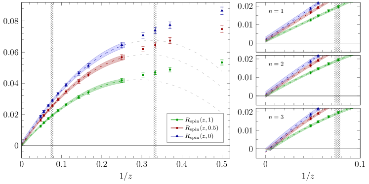
Figure 6: Asymptotic behaviour of the spin splitting observable $R_{\rm spin}(z,\theta_{0})$ together with a quadratic unconstrained (and weighted) fit including data at $1/z\leq 1/4$. In the right panels we compare the static extrapolation in the asymptotic scaling region for a linear ($n=1$), quadratic ($n=2$) and cubic ($n=3$) polynomial fit ansatz.

As can be inferred from figure 6, our spin splitting observable $R_{\rm spin}(z,\theta_{0})$ shows the expected asymptotic behaviour towards the $1/z\to 0$ limit, where it has to vanish due to the heavy-quark spin symmetry. Opposed to the case of the static axial current, data for the corresponding RGI matrix element, $X^{\rm spin}_{\rm RGI}$, are not available for the two-flavour theory. Hence, we refrain from studying the static limit of our data in the form of applying eq. (22) via (16) to $R_{\rm spin}/C_{\rm spin}$, as we did for the axial and vector meson decay constants in the previous paragraph. Rather, we studied different static extrapolations using a linear ($n=1$, $z\geq 13$), quadratic ($n=2$, $z\geq 4$) and cubic ($n=3$, $z\geq 3$) fit ansatz for the static extrapolation. They are presented for better visibility in the asymptotic region only (right panel of figure 6). The left panel shows the $n=2$ case with all available data points; the fit ansaetze are able to describe the data very well, and its behaviour confirms the HQET expectation.

3.3 Results without perturbative conversion functions

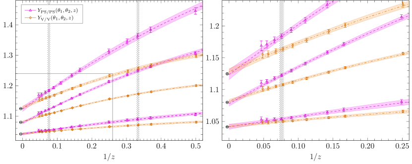
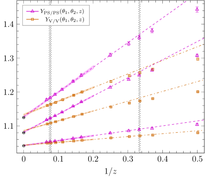
Figure 7: Extrapolations of $Y_{\rm PS/PS}(z,\theta_{1},\theta_{2})$ and $Y_{\rm V/V}(z,\theta_{1},\theta_{2})$ to the static limit for all three combinations of $(\theta_{1},\theta_{2})$. The results are listed in table 2. The right panel shows a scaled excerpt of the heavy quark mass region. Black data points indicate the continuum results of the corresponding quantity at static order of HQET. Its continuum extrapolation is displayed in figure 2. For comparison, the lower panel displays an extrapolation with just a linear function in $1/z$ for $1/z\leq 0.2$ that leads to an equally well confirmation of the HQET expectation.

	static limit in QCD		static HQET	static limit in QCD		static HQET
$(\theta_{1},\theta_{2})$	$Y_{\rm PS/PS}$	$Y_{\rm V/V}$	$R_{X}^{\rm stat}$	$R_{f}$	$R_{k}$	$R_{f}^{\rm stat}$
$(0,0.5)$	$1.0417(20)$	$1.0424(15)$	$1.0414(4)$	$1.222(11)$	$1.220(11)$	$1.2245(16)$
$(0.5,1)$	$1.0796(22)$	$1.0841(16)$	$1.0800(5)$	$1.760(21)$	$1.759(21)$	$1.7234(34)$
$(0.0,1)$	$1.1247(42)$	$1.1300(29)$	$1.1248(8)$	$2.143(46)$	$2.142(46)$	$2.1107(64)$

Table 2: Results of static extrapolations of decay constant ratios in continuum QCD and its corresponding non-perturbative continuum extrapolation results in the static effective theory.

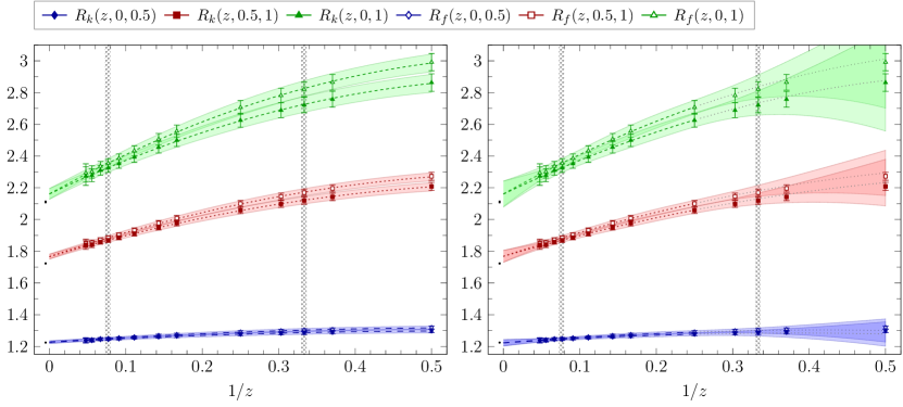
Figure 8: Static extrapolations of $R_{f}(z,\theta_{1},\theta_{2})$ and $R_{k}(z,\theta_{1},\theta_{2})$ for all three combinations of $(\theta_{1},\theta_{2})$. In the left panel, all data points enter the static extrapolations, whereas in the right panel only those with $1/z\leq 1/4$ contribute. The results are listed in table 2. Black data points indicate the continuum results of the corresponding quantity at static order of HQET, cf. eq. (18).

We now turn our attention to quantities that do not depend on any conversion functions and as such are free of any influence of perturbative uncertainties; they thus are expected to exhibit an unambiguous static extrapolation compatible with their heavy quark mass expansion. In most cases we find that a fit function such as

$$\Omega^{\rm QCD}(L,M,0) =\upsilon_{0}+\upsilon_{1}z^{-1}+\upsilon_{2}z^{-2}$$ (27)

models their $z$-dependence in the continuum limit very well over the whole region of available heavy quark mass values.

Ratios of currents

As prototype observables, we first consider and probe eq. (18c), viz.

$$Y_{\rm PS/PS}(z,\theta_{1},\theta_{2}) =R_{X}^{\rm stat}(\theta_{1},\theta_{2})+{\rm O}(1/z)\;,$$

$$Y_{\rm V/V}(z,\theta_{1},\theta_{2}) =R_{X}^{\rm stat}(\theta_{1},\theta_{2})+{\rm O}(1/z)\;,$$ (28)

where — again owing to the heavy-quark spin symmetry — the static extrapolation of the ratio of effective vector current matrix elements computed at different kinematical parameters, $Y_{\rm V/V}(z,\theta_{1},\theta_{2})$, is expected to agree in the limit $1/z\to 0$ with the associated ratio in the pseudoscalar channel, $Y_{\rm PS/PS}(z,\theta_{1},\theta_{2})$, and to approach the common, non-trivial leading-order HQET prediction $R_{X}^{\rm stat}(\theta_{1},\theta_{2})$, which denotes the corresponding ratio of matrix elements computed by replacing the relativistic fields by the static ones.

Performing an unconstrained extrapolating fit of all data points ($z\geq 2$), according to the fit ansatz (27), gives an asymptotic behaviour as depicted in figure 7 for the three available $\theta$-combinations. The black circles (slightly moved to the left towards negative $1/z$ for ease of presentation) represent the results for the ratio of static-order HQET matrix elements, $R_{X}^{\rm stat}(\theta_{1},\theta_{2})$. As usual throughout this work, all data points were extrapolated to the continuum limit first; in particular, the continuum extrapolation of $R_{X}^{\rm stat}(\theta_{1},\theta_{2})$ is presented in the left panel of figure 2 and its numerical values can be read off together with the results of the static extrapolations from table 2.

In contrast to the decay constant discussed in the previous subsection, the comparison in figure 7 illustrates a very good agreement between the static extrapolations of the results on $Y_{\rm V/V},Y_{\rm PS/PS}$ and the numbers for $R_{X}^{\rm stat}$, computed to even much higher statistical accuracy directly in the static approximation. Moreover, from the fits in the lower panel of the figure one reads off an equally excellent agreement with the HQET expectation from an extrapolation with just a linear function in $1/z$ for $z\geq 5$ ($1/z\leq 0.2$). These findings not only demonstrate the correctness of the effective theory itself, but also strongly advocate such observables, which are not affected by any perturbative imperfections deriving from conversion functions, as most promising candidates for observables for use in a non-perturbative strategy for matching HQET to QCD in the spirit of Heitger:2003nj . Two additional observations worth to be mentioned are: a) the error for all three combinations of $(\theta_{1},\theta_{2})$ grows with increasing $\theta_{2}^{2}-\theta_{1}^{2}$ in a similar way for all three observables; b) also the $1/z$-terms, i.e., the slope at $1/z=0$, grows with that difference. These features also hold true for the quantities considered next and in principle can serve as further helpful criteria for a sensible choice of matching observables.

Ratios of boundary-to-boundary matrix elements

At next, we look at the static extrapolation of the quantities entering the prediction (18a). Compared to observables studied before, the QCD data points obtained in the vector ($R_{k}$) and pseudoscalar channel ($R_{f}$) lie quite close to each other already at finite quark mass. From figure 8 (left panel) one concludes that superficially the quadratic fit ansatz (27) very well represents the data points, which approach a (due to spin symmetry) common HQET limit for the three $\theta$-combinations. Note that the static HQET results for $R_{k}$ and $R_{f}$, independently computed in the continuum limit from different simulations, have not been constrained to be equal, but their agreement is just excellent though. However, only the extrapolation for the combination $(\theta_{1},\theta_{2})=(0,0.5)$ leads to the correct result in the static limit, $R_{k}=R_{f}$, represented in the figure by the leftmost black data points. The results for this particular static extrapolation and the corresponding HQET results are given in table 2.

This partial mismatch of the results from extrapolations of the QCD data over the whole available $z$-range down to $z=2$ ($1/z=0.5$) with the HQET predictions should be taken as a warning that the validity of the HQET-inspired $1/m_{\rm h}$-expansion of heavy-light QCD obeservables in the large-mass regime can not be tacitly trusted down to the charm quark scale or below. In fact, if we restrict the fits to include data points for $1/z<0.26$ only, as done in the previous section, we obtain a static extrapolation as shown in the right panel of figure 8, where the static numbers can be seen to be covered by the error of the extrapolation results. An even further restriction of the fit interval to $1/z<0.1$ would easily allow for a feasible linear interpolating fit including the HQET result as a constraint. Here, extending those fits to the lower $z$’s that were excluded yields only mild deviations of about 1$\sigma$ between the fit functions and the data points, though, but this may also be more pronounced for other observables. Turning the argument around, an interpolating fit somewhat arbitrarily extended, at fixed polynomial degree, to include data below the charm region ($z=2$), which appears to give a good description of the data, can lead to an underestimation of the error of the static extrapolation and thereby pretend to miss the HQET prediction.

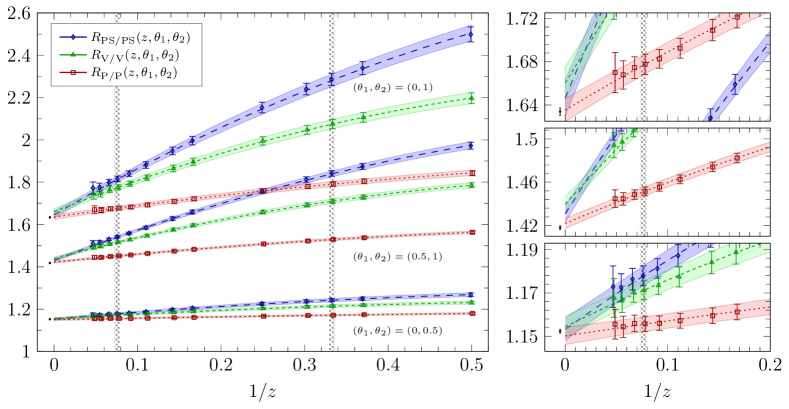
Figure 9: Static extrapolations of $R_{\rm PS/PS}(z,\theta_{1},\theta_{2})$, $R_{\rm V/V}(z,\theta_{1},\theta_{2})$ and $R_{\rm P/P}(z,\theta_{1},\theta_{2})$ for all three combinations of $(\theta_{1},\theta_{2})$ in comparison to their HQET counterparts after taking the continuum limit in the static effective theory (these data points are slightly shifted for better readability). The results are listed in table 2. The right panel shows a scaled excerpt of the heavy quark mass region individually for the three available $(\theta_{1},\theta_{2})$-combinations such that error bars of the HQET results become visible.

	static limit in QCD			static HQET
$(\theta_{1},\theta_{2})$	$R_{\rm PS/PS}$	$R_{\rm V/V}$	$R_{\rm P/P}$	$R_{\rm PS}^{\rm stat}$
$(0,0.5)$	$1.1532(52)$	$1.1545(49)$	$1.1502(40)$	$1.1523(9)$
$(0.5,1)$	$1.4309(76)$	$1.4399(65)$	$1.4219(47)$	$1.4180(18)$
$(0.0,1)$	$1.647(17)$	$1.660(15)$	$1.635(11)$	$1.6339(34)$

Table 3: Results for static extrapolations of $R_{\rm PS/PS}$, $R_{\rm V/V}$ and $R_{\rm P/P}$ in continuum QCD as displayed in figure 9 and its corresponding non-perturbative continuum extrapolation results in the static effective theory.

Ratios of boundary-to-bulk matrix elements

Finally, we check the static extrapolation of eq. (18b). The HQET results for $R_{\rm PS}^{\rm stat}(\theta_{1},\theta_{2})$ follow from the continuum extrapolation presented in figure 2. Their values are given in table 3, together with the results that stem from a static extrapolation of the (continuum) QCD observables $R_{\rm PS/PS}$, $R_{\rm V/V}$ and $R_{\rm P/P}$ as defined in eq. (9). Once more, the data sets themselves are very well represented by a quadratic polynomial fit ansatz over the whole range of available data points, whereas the static HQET result (common to all three QCD observables, again due to spin symmetry) is only met for the $\theta$-combination $(\theta_{1},\theta_{2})=(0,0.5)$ as in the foregoing case of ratios of boundary-to-boundary matrix elements. Accordingly, the same discussion (and warning) carries over literally here, except for $R_{\rm P/P}$ that very well extrapolates to the HQET result for all $\theta$-combinations studied. Since the errors on the data points for $R_{\rm P/P}$ stay roughly the same when going from the scale of the b-quark mass down to $z=2$, the slight mismatch in the other cases may likely be attributed partly to statistical effects.

4 Conclusions

We have studied the asymptotic large-mass behaviour of heavy-light meson observables in lattice QCD with two massless dynamical sea quarks, in a small volume of linear extent $L_{1}\approx 0.4\,{\rm fm}$ and for heavy quark mass values within a range from beyond the b- to below the c-quark scale, in order to confront them with their HQET predictions.

Having taken the continuum limit in all parts of our entirely non-perturbative calculations on both the QCD and the HQET side and subsequently performed unconstrained static extrapolations along the limit $z=L_{1}M_{\rm h}\to\infty$, in most cases we generically find (within the numerical precision on our results with errors at the few-% level) a very satisfactory — sometimes an even excellent — agreement between the large-mass asymptotics of the QCD observables and their expected leading-order HQET limits.

Moreover, the overall quality of the polynomial fits in $1/z$ to the heavy quark mass dependence of the (continuum) heavy-light QCD observables convincingly demonstrates that the theory is very well described by simple $1/m_{\rm h}$-corrections to the static limit of the effective theory. In particular, for $1/z\lesssim 0.1$ our extrapolating fits to the HQET predictions can consistently be modeled by functions linear in $1/z$. We are thus led to conclude that the effective theory is very well tested and that the regime with $1/z\lesssim 0.1$, which is a key ingredient to the finite-volume matching part of the ALPHA Collaboration’s B-physics programme based on HQET non-perturbatively renormalized and matched to QCD at ${\rm O}(1/m_{\rm h})$ Heitger:2003nj ; Blossier2010 ; Blossier2010a ; Blossier:2010mk ; Blossier:2012qu ; Bernardoni:2013xba ; Bernardoni:2014fva ; Bernardoni:2015nqa , lies very well within the applicability domain of HQET. This is, for instance, also in line with the onset of the linear behaviour reported in the tree-level study DellaMorte:2013ega of the $1/z$-dependence of the HQET parameters contributing to the full set of heavy-light flavour currents in HQET at ${\rm O}(1/m_{\rm h})$. Alltogether, these findings are very reassuring, since they imply that in the finite-volume setup of the aforementioned non-perturbative matching strategy between HQET and QCD, higher-order corrections beyond the ${\rm O}(1/m_{\rm h})$ ones already included can be expected to be suppressed by a factor of about $10$.

A prominent exception to this favourable outcome of our tests of HQET consists in the large-mass asymptotics of the small-volume heavy-light axial vector and vector meson decay constants, which fails to meet the leading-order HQET prediction in the static limit. But, as argued in section 3.2, rather than interpreting this as an inherent shortcoming of HQET being not an appropriate and predictive effective theory of QCD, one should take this as an advice that it is generally safer not to use conversion functions such as $C_{\rm PS},C_{\rm V}$ (which inevitably enter in a consistent comparison of QCD and HQET decay constants) from perturbation theory, even if they are determined at three-loop accuracy, i.e., with relative errors of order $\bar{g}^{6}(m_{\ast})$ at some intrinsic mass scale $m_{\ast}$; e.g., their perturbative convergence appears to be relatively poor still at the b-quark scale. Otherwise, the combination of non-perturbative QCD data with the mass dependence via perturbative matching functions (encoding the running in HQET) to recover the correct HQET limit can easily lead to inconsistencies between QCD and non-perturbatively computed matrix elements in the effective theory. For the decay constant, we encounter a systematic effect of up to $\sim 5\%$ from relying on perturbative running in the effective theory. Therefore, we consider this as a warning when, e.g., the physical (i.e., large-volume) B-meson decay constant is being extracted involving interpolations between QCD data below the b-scale and the static limit, and advocate to perform the matching entirely non-perturbatively.

As already noted earlier in Sommer:2010ic , a more quantitative understanding of this deficiency can be gained from the relative error that results from a truncation of the perturbative matching expression at $l$-loop order, viz.

$${\Delta(C_{\rm PS})\over C_{\rm PS}} \;\propto\;\big{[}\bar{g}^{2}(m_{\ast})\big{]}^{l}\;\sim\;\left[{1\over 2b_{0}\ln\big{(}m_{\ast}/\Lambda\big{)}}\right]^{l}\;\;\stackrel{{\scriptstyle m_{\ast}\gg\Lambda}}{{\gg}}\;\;{\Lambda\over m_{\ast}}\;.$$ (29)

I.e., since this perturbative uncertainty only decreases logarithmically as $m_{\ast}$ becomes large, at some point it starts to dominate over the power correction that one needs to include at next-to-leading order in the HQET expansion for precision physics at the b-quark mass scale. This underlines once more that with an only perturbative conversion function, a consistent next-to-leading order expansion with errors decreasing as $1/m_{\rm h}^{2}$ can not be achieved.

Another interesting aspect of our work is that the continuum extrapolations of the HQET observables, such as those presented in figure 2 of section 3.1 for two discretizations of the static quark, provide strong numerical evidence that an universal continuum limit of the static effective theory exists and that the non-perturbative renormalizability of HQET along the finite-volume matching strategy of ref. Heitger:2003nj can be established indeed.

Finally, let us emphasize that exploring the size of the higher-order corrections in our QCD observables to test HQET non-perturbatively may also readily serve as a guide so single out preferred choices among observables, suitable for a specific HQET-QCD matching problem in question, that have only small ${\rm O}(1/m_{\rm h}^{2})$ contributions. In addition to that, any flexibility in having different matching equations made of different observables to determine the same (set of) HQET parameters enables further useful checks in actual computations, because the final results should be independent of any specific but sensible choice of matching equations and kinematical parameters (such as $T/L$, $x_{0}$ and the $\theta$’s) entering them, up to small ${\rm O}(1/m_{\rm h}^{2})$ corrections.

Appendix A Definitions

Here we provide the definitions of the observables of this study in terms of the traditional notation for Schrödinger functional (SF) correlation functions. We do not repeat all details here; for explicit expression for SF heavy-light meson correlators in lattice QCD as well as in the static limit of lattice HQET, the reader may, e.g., consult Heitger:2003nj ; DellaMorte:2006cb ; Kurth:2000ki ; DellaMorte:2013ega .

QCD observables

For the effective masses we use SF correlation functions $f_{\rm X}$ with bulk insertions of ${\rm O}(a)$ improved heavy-light currents (cf. section 2) in the pseudoscalar and vector channel and define

$$\Gamma_{\rm PS} =\left.-\widetilde{{\partial_{0}}}\ln f_{\rm A}^{\rm I}(x_{0})\right|_{x_{0}=\tfrac{T}{2}}\;, \Gamma_{\rm P} =\left.-\widetilde{{\partial_{0}}}\ln f_{\rm P}(x_{0})\right|_{x_{0}=\tfrac{T}{2}}\;,$$

$$\Gamma_{\rm V} =\left.-\widetilde{{\partial_{0}}}\ln k_{\rm V}^{\rm I}(x_{0})\right|_{x_{0}=\tfrac{T}{2}}\;.$$ (30)

Effective decay constants associated with these correlators as well as suitable ratios thereof require renormalization and are given by

$$Y_{\rm PS} \equiv+Z_{\rm A}(1+\tfrac{1}{2}b_{\rm A}am_{\rm q,h})\dfrac{f_{\rm A}^{\rm I}(T/2)}{\sqrt{f_{1}}}\;, Y_{\rm V} \equiv-Z_{\rm V}(1+\tfrac{1}{2}b_{\rm V}am_{\rm q,h})\dfrac{k_{\rm V}^{\rm I}(T/2)}{\sqrt{k_{1}}}\;,$$ (31)

$$R_{\rm PS/P} \equiv-\dfrac{Z_{\rm A}(1+\tfrac{1}{2}b_{\rm A}am_{\rm q,h})}{Z_{{\rm P},{\rm RGI}}(1+\tfrac{1}{2}b_{\rm P}am_{\rm q,h})}\dfrac{f_{\rm A}^{\rm I}(T/2)}{f_{\rm P}(T/2)}\;, R_{\rm PS/V} \equiv-\dfrac{Z_{\rm A}(1+\tfrac{1}{2}b_{\rm A}am_{\rm q,h})}{Z_{\rm V}(1+\tfrac{1}{2}b_{\rm V}am_{\rm q,h})}\dfrac{f_{\rm A}^{\rm I}(T/2)}{k_{\rm V}^{\rm I}(T/2)}\;.$$ (32)

The renormalization constants $Z_{\rm X}$, $\rm X={\rm A},{\rm V},{\rm P}$, are known non-perturbatively in two-flavour QCD; as in our earlier work Fritzsch:2010aw , $Z_{\rm A}$ and $Z_{\rm V}$ have been taken from DellaMorte:2008xb , while $Z_{{\rm P},{\rm RGI}}$ is available through the scale dependent renormalization factor $Z_{\rm P}$ computed in refs. DellaMorte:2005kg ; Blossier:2012qu . The improvement coefficients $b_{\rm X}$ (multiplying the bare subtracted heavy quark mass) are known to one-loop order of perturbation theory and can be found in Sint:1997jx .

The spin splitting observable, however, is constructed from a ratio of SF boundary-to-boundary correlators with pseudoscalar and vector channel composite fields, free of any improvement coefficient and renormalization factor:

$$R_{\rm spin} \equiv\tfrac{3}{4}\ln\left[f_{1}/k_{1}\right]\;.$$ (33)

As already explained in the main text, the foregoing finite-volume observables have been computed for one fermionic phase angle out of $\theta_{0}\in\{0,0.5,1\}$. To enlarge the variety in probing QCD and HQET at different kinematics, it remains to specify the observables that depend on two such angles. Here we build them from SF correlation functions with different $\theta$’s, i.e.,

$$R_{\rm PS/PS}(\theta_{1},\theta_{2}) =\left.\frac{f_{\rm A}^{\rm I}(x_{0},\theta_{1})}{f_{\rm A}^{\rm I}(x_{0},\theta_{2})}\right|_{x_{0}=T/2}\;, R_{f}(\theta_{1},\theta_{2}) =\frac{f_{1}(\theta_{1})}{f_{1}(\theta_{2})}\;,$$

$$R_{\rm V/V}(\theta_{1},\theta_{2}) =\left.\frac{k_{\rm V}^{\rm I}(x_{0},\theta_{1})}{k_{\rm V}^{\rm I}(x_{0},\theta_{2})}\right|_{x_{0}=T/2}\;, R_{k}(\theta_{1},\theta_{2}) =\frac{k_{1}(\theta_{1})}{k_{1}(\theta_{2})}\;,$$

$$R_{\rm P/P}(\theta_{1},\theta_{2}) =\left.\frac{f_{\rm P}(x_{0},\theta_{1})}{f_{\rm P}(x_{0},\theta_{2})}\right|_{x_{0}=T/2}\;,$$ (34)

where in practice we have chosen to extract them from our simulations for the non-trivial combinations $(\theta_{1},\theta_{2})\in\{(0,0.5),(0.5,1),(0,1)\}$. Again, renormalization factors drop out in these ratios.

HQET observables

Among the QCD observables defined above depending on a single $\theta$-angle, only the effective decay constants in eq. (31) possess a (common) non-trivial static limit, which is given by

$$X(\theta)=\left.\frac{f_{\rm A}^{\rm stat}(x_{0},\theta)}{\sqrt{f_{1}^{\rm stat}(\theta)}}\right|_{x_{0}=T/2}$$ (35)

up to renormalization factors (cf. subsection 2.5) to be discussed in appendix C, while the ratios in (32) approach $1$ as a consequence of the heavy-quark spin symmetry that entails pseudoscalar and vector channels to coincide. The ratios in eq. (A) depending two $\theta$-angles, on the other hand, approach in the static limit one of the following observables at static order of HQET:

$$R_{\rm PS}^{\rm stat}(\theta_{1},\theta_{2}) =\left.\frac{f_{\rm A}^{\rm stat}(x_{0},\theta_{1})}{f_{\rm A}^{\rm stat}(x_{0},\theta_{2})}\right|_{x_{0}=T/2}\;, R_{f}^{\rm stat}(\theta_{1},\theta_{2}) =\frac{f_{1}^{\rm stat}(\theta_{1})}{f_{1}^{\rm stat}(\theta_{2})}\;,$$ (36)

$$R_{X}^{\rm stat}(\theta_{1},\theta_{2}) =\frac{X(\theta_{1})}{X(\theta_{2})}\;.$$ (37)

The corresponding static-light correlation functions $f_{\rm A}^{\rm stat}$ and $f_{1}^{\rm stat}$ entering in these expressions have first been defined in Kurth:2000ki .

Appendix B Conversion functions

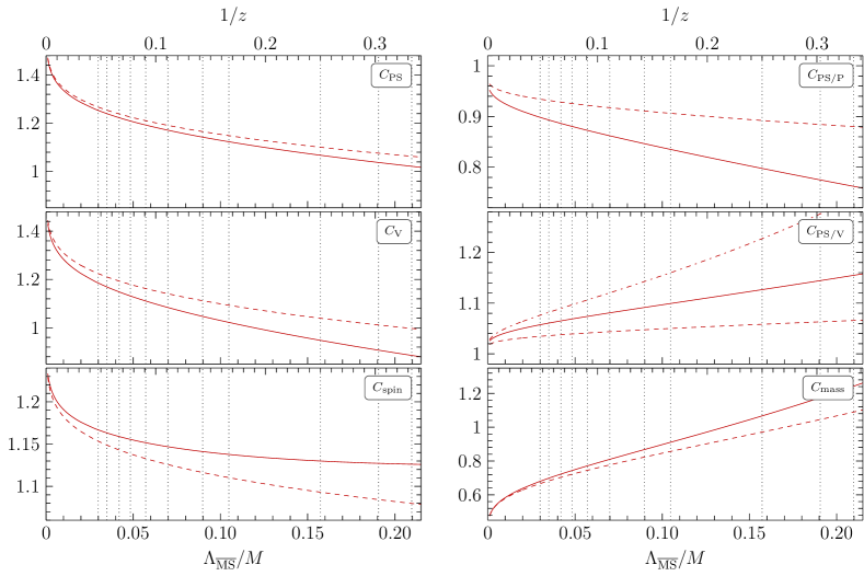
Figure 10: HQET-QCD conversion functions $C_{\rm X}$ for heavy-light currents as described in the text. The solid and dashed curves correspond to the three-loop and two-loop order anomalous dimensions in the matching scheme, respectively. In the case of $C_{{\rm PS}/{\rm V}}$ (middle panel on the right), the four-loop expression, which is known from Bekavac2010 , is also included as dash-dotted curve. Comparing the curves for different loop orders suggests that perturbation theory converges rather slowly. Vertical dotted lines indicate the fixed values of $z=L_{1}M$ used in our study.

In this section we summarize the expressions of the perturbative conversion functions $C_{\rm X}$, $\rm X\in\{{\rm PS},{\rm V},{\rm spin},{\rm PS}/{\rm P},{\rm PS}/{\rm V},{\rm mass}\}$, that have been employed to compare our non-perturbatively renormalized observables in QCD to their counterparts in HQET. They are computed and parameterized in the so-called matching scheme, which has been introduced in Heitger:2003xg and specified in appendix B of Heitger:2004gb (see also Sommer:2010ic for another detailed discussion). Our formulae for all relevant operators below refer to the two-flavour theory and are based on their anomalous dimensions known up to three-loop order in continuum perturbation theory Tarrach:1980up ; Shifman:1987sm ; Politzer:1988wp ; Gray:1990yh ; Eichten:1990vp ; Falk:1991pz ; Ji:1991pr ; Broadhurst:1991fz ; Gimenez:1991bf ; HQET:sigmabI ; HQET:sigmabII ; Chetyrkin:2003vi ; Grozin:2007fh , to be combined with the matching coefficients between QCD and the effective theory up to two loops Eichten:1989zv ; Eichten:1989kb ; Eichten:1990vp ; Broadhurst:1994se ; Grozin:1998kf , see appendix B of Heitger:2004gb . In order to judge the impact of the order of the perturbative expansion on this comparison between QCD and HQET, introduced by the conversion functions $C_{\rm X}$ as far as they enter the observables under study, we evaluate the $C_{\rm X}$ including the two-loop and three-loop anomalous dimensions (together with the respective matching coefficients in one- and two-loop accuracy) separately. In both cases we use the four-loop beta-function for the coupling 'tHooft:1973mm ; Gross:1973id ; Caswell:1974gg ; Tarasov:1980au ; vanRitbergen:1997va ; Czakon:2004bu , while the conversion function for effective masses involves the quark mass anomalous dimension $\tau$ at four-loop Chetyrkin:1997dh ; Vermaseren:1997fq ; Czakon:2004bu .

Moreover, thanks to the three-loop calculation of the matching coefficients for the heavy-light currents available from Bekavac2010 , the anomalous dimensions of ratios of currents become effectively known to four-loop order in the matching scheme, because the unknown four-loop anomalous dimensions of the currents themselves cancel out in the difference of anomalous dimensions contributing to these ratios. As an example, we therefore also include the conversion function $C_{{\rm PS}/{\rm V}}$ of the ratio of axial vector ($A_{0}$) to vector ($V_{k}$) currents at four-loop accuracy in our study.

Since so far only $C_{\rm PS}$ for the $N_{\rm f}=2$ theory was given earlier in DellaMorte:2006sv , we here list the parametrization of all conversion functions $C_{\rm X}$ entering this study that were obtained along the lines detailed in appendix B of Heitger:2004gb . They are expressed as smooth functions in terms of the variable

$$x \equiv 1\left/\ln\left[M/\Lambda_{\overline{{\rm MS}}}\right]\right.\;, \dfrac{M}{\Lambda_{\overline{{\rm MS}}}} =\dfrac{z}{L_{1}\Lambda_{\overline{{\rm MS}}}}\;,$$ (38)

with the product $L_{1}\Lambda_{\overline{{\rm MS}}}=0.629(36)$ in the two-flavour theory taken from Fritzsch:2012wq and $M$ denoting the renormalization group invariant (RGI) heavy quark mass as in the main text. The functions decompose into a pre-factor which encodes the leading logarithmic asymptotics (if any) as $x\rightarrow 0$, multiplied by a polynomial in $x$ which reflects the perturbative order of the underlying anomalous dimension in conjunction with the associated matching coefficients.

$$C_{\rm PS}(x) =\begin{cases}\begin{array}[]{ll}x^{\gamma^{\rm PS}_{0}/(2b_{0})}\left\{1-0.107x+0.093x^{2}\right\}&\;\text{: 2-loop }\gamma^{\rm PS}\\[2.5pt] x^{\gamma^{\rm PS}_{0}/(2b_{0})}\left\{1-0.118x-0.010x^{2}+0.043x^{3}\right\}&\;\text{: 3-loop }\gamma^{\rm PS}\end{array}\end{cases}\;,$$ (39)

$$C_{\rm V}(x) =\begin{cases}\begin{array}[]{ll}x^{\gamma^{\rm V}_{0}/(2b_{0})}\left\{1-0.239x+0.153x^{2}\right\}&\text{: 2-loop }\gamma^{\rm V}\\[2.5pt] x^{\gamma^{\rm V}_{0}/(2b_{0})}\left\{1-0.266x-0.178x^{2}+0.193x^{3}\right\}&\text{: 3-loop }\gamma^{\rm V}\end{array}\end{cases}\;,$$ (40)

$$C_{\rm spin}(x) =\begin{cases}\begin{array}[]{ll}x^{\gamma^{\rm spin}_{0}/(2b_{0})}\left\{1+0.043x+0.09x^{2}\right\}&\text{: 2-loop }\gamma^{\rm spin}\\[2.5pt] x^{\gamma^{\rm spin}_{0}/(2b_{0})}\left\{1+0.044x+0.179x^{2}-0.099x^{3}\right\}&\text{: 3-loop }\gamma^{\rm spin}\end{array}\end{cases}\;,$$ (41)

$$C_{\rm PS/P}(x) =\begin{cases}\begin{array}[]{ll}1-0.266x+0.123x^{2}&\,\text{: 2-loop }\gamma^{\rm PS,P}\\[2.5pt] 1-0.293x-0.304x^{2}+0.284x^{3}&\,\text{: 3-loop }\gamma^{\rm PS,P}\end{array}\end{cases}\;,$$ (42)

$$C_{{\rm PS}/{\rm V}}(x) =\begin{cases}\begin{array}[]{ll}1+0.136x-0.052x^{2}&\quad\;\text{: 2-loop }\gamma^{\rm PS,V}\\[2.5pt] 1+0.142x+0.250x^{2}-0.148x^{3}&\quad\;\text{: 3-loop }\gamma^{\rm PS,V}\\[2.5pt] 1+0.135x+0.323x^{2}+0.614x^{3}-0.436x^{4}&\quad\;\text{: 4-loop }\gamma^{\rm PS,V}\end{array}\end{cases}\;,$$ (43)

$$C_{\rm mass}(x) =\begin{cases}\begin{array}[]{ll}x^{\,d_{0}/(2b_{0})}\left\{1+0.373x+0.176x^{2}\right\}&\,\text{: 2-loop }\tau\\[2.5pt] x^{\,d_{0}/(2b_{0})}\left\{1+0.287x+0.752x^{2}+0.011x^{3}\right\}&\,\text{: 3-loop }\tau\end{array}\end{cases}\;.$$ (44)

The functional dependence of the $C_{\rm X}$ on $\Lambda_{\overline{{\rm MS}}}/M$ is shown in figure 10. The solid curves represent the matching functions to (in most cases) highest available perturbative accuracy, i.e., corresponding to three-loop anomalous dimensions of the heavy-light currents involved and the four-loop beta-function. The dashed curves are those obtained with two-loop anomalous dimensions only. For illustration, we plot as vertical dotted lines the values of $z$ which have been fixed in order to non-perturbatively compute our test observables. In the exemplary case of the ratio of pseudoscalar to vector currents, $C_{{\rm PS}/{\rm V}}$, which we are able to consider even up to the maximally available four-loop precision (dash-dotted curve in the middle-right panel of figure 10), one observes an increase in the size of correction when going from two- to three- and three- to four-loop order. This is in accordance with the conclusion of the authors of Bekavac2010 that the perturbative series for this ratio of currents “converges very slowly at best”. We finally remark that, since the previous expressions derive from continuum perturbation theory, the functions $C_{\rm X}$ must be properly attached as factors to the HQET-QCD test observables in question after the lattice results on them have been extrapolated to the continuum limit, cf. section 2.5.

Appendix C Further details and tables

Tree-level improvement

Even though our simulations are performed at rather fine lattice spacings, one ultimately encounters mass-dependent cutoff effects, which essentially grow with the heavy quark mass, i.e., to some power of $z\times a/L=aM$ in the non-perturbatively ${\rm O}$ improved theory. To attenuate these effects, we also apply perturbative improvement to some of our lattice observables under consideration. Here we restrict ourselves to tree-level improvement (TLI), which for a generic test observable $\Omega$ amounts to the replacement

$$\Omega(\bar{g}^{2},a/L,z)\;\to\;\Omega^{(0)}(\bar{g}^{2},a/L,z) =\frac{\Omega(\bar{g}^{2},a/L,z)}{1+\delta^{(0)}_{\Omega}(a/L,z)}\;,$$

$$\delta^{(0)}_{\Omega}(a/L,z) =\frac{\Omega^{\rm tree}(a/L,z)-\Omega^{\rm tree}(0,z)}{\Omega^{\rm tree}(0,z)}\;,$$ (45)

and thereby removes all the ${\rm O}\left((\frac{a}{L})^{n}\right)$ effects to produce classically perfect observables. For additional details on the actual extraction of the improvement terms $\delta^{(0)}_{\Omega}$, see appendix D of Blossier2010 . Besides its obvious dependence on $z$ and $a/L$, $\delta^{(0)}_{\Omega}$ also depends on the kinematical setup of the Schrödinger functional, inherited from the observable itself. These are the choice of boundary gauge field, the ratio $T/L$ and the fermionic periodicity angles involved in the definition of $\Omega$. Except for $\Omega\in\{R_{\rm PS/PS},R_{\rm V/V},R_{\rm P/P},R_{1},R_{f},R_{k}\}$, where TLI has not been accounted for, and observables such as $R_{\rm spin}$, where it vanishes exactly, the presented results always correspond to the tree-level improved quantities.

We furthermore remark that before any continuum limit in QCD and HQET is taken numerically, we use the data from appendix B of Blossier:2012qu to correct for small deviations in our observables from the renormalized (i.e., constant physics) trajectory at $(L_{1}m_{\rm l},\bar{g}^{2}(L_{1}))=(0,4.484)$. The associated errors are propagated quadratically.

Special case: Axial current renormalization

We add some remarks about the continuum extrapolation of the RGI static decay constant as defined in eq. (17), because we need to fully specify the renormalization scheme applied.

The total renormalization factor to obtain the RGI matrix element of the static axial current, $X_{\rm RGI}$, from the bare matrix element, $X_{\rm bare}$, decomposes into

$$Z^{\rm stat}_{\rm A,RGI}(g_{0},\theta) \equiv\left[\frac{Z^{\rm stat}_{\rm A,RGI}}{Z^{\rm stat}_{\rm A}(\mu)}\cdot Z_{\rm A}^{\rm stat}(g_{0},a\mu)\right]_{\mu=L_{1}^{-1}}^{(\theta,\rho)}=\left[\frac{Z^{\rm stat}_{\rm A,RGI}}{Z^{\rm stat}_{\rm A}(\mu)}\frac{X(0,a\mu)}{X_{\rm bare}(g_{0},a\mu)}\right]_{\mu=L_{1}^{-1}}^{(\theta,\rho)}\;.$$ (46)

As indicated here, the universal part $Z^{\rm stat}_{\rm A,RGI}/Z^{\rm stat}_{\rm A}(\mu)$, which links a renormalized matrix element of the static axial current at a renormalization scale $\mu$ to the RGI one, is defined within the massless SF scheme for vanishing boundary field and $(\theta,\rho=T/L)=(0.5,1)$ non-perturbatively and in the continuum limit. For the particular scale $\mu=L_{1}^{-1}$ corresponding to the physical volume employed in the present work, $Z^{\rm stat}_{\rm A,RGI}/Z^{\rm stat}_{\rm A}(\mu)$ has been re-computed from the two-flavour data of ref. DellaMorte:2006sv to yield the estimate quoted in (17). (Note that in DellaMorte:2006sv , the universal ratio was denoted as $\Phi_{\rm RGI}/\Phi(\mu)$). In the definition of the scale dependent renormalization factor itself, $Z_{\rm A}^{\rm stat}(g_{0},a\mu)$, the tree-level normalization factor $X(0,L/a)$ enters at the respective values of $(\theta,\rho)$ such that $Z_{\rm A}^{\rm stat}$ approaches one in the limit $g_{0}\to 0$, cf. Heitger:2003xg . In fact, as we always have $\rho=T/L=1$ in the present work, too, we can take the continuum limit according to

$$X_{\rm RGI}(\theta_{0}) =\lim_{L_{1}/a\to 0}\,Z^{\rm stat}_{\rm A,RGI}(g_{0},\theta)\,X_{\rm bare}(g_{0},L_{1}/a,\theta_{0})$$

$$\equiv\lim_{L_{1}/a\to 0}\,\frac{Z^{\rm stat}_{\rm A,RGI}}{Z^{\rm stat}_{\rm A}(\mu)}\,X_{\rm R}(\mu)\;,$$ (47)

with the particular values $\theta_{0}\in\{0,0.5,1\}$ and $\theta=0.5$. The second equality in (47) picks up the notation of eq. (17), and the results are listed in table 1. Finally, let us point out that its total error is dominated by the error of the universal continuum factor for the non-perturbative running, $Z^{\rm stat}_{\rm A,RGI}\big{/}Z^{\rm stat}_{\rm A}(\mu)$ (as quoted in (17)), and that this part of the error is only to be accounted for after $X_{\rm RGI}$ has been extrapolated to the continuum limit.

Tables

	$L_{1}/a$	$20$	$24$	$32$	$40$
$z$	$\beta$	$6.1569$	$6.2483$	$6.4574$	$6.6380$
$\approx 0$	$\kappa_{\rm l}\approx\kappa_{\rm crit}$	$0.1360536$	$0.1359104$	$0.1355210$	$0.1351923$
$2.0$	$\kappa(z,\beta)$	$0.1344153854$	$0.1345754522$	$0.1345486577$	$0.1344246956$
$2.7$	$\kappa(z,\beta)$	$0.1338267897$	$0.1340982540$	$0.1342031414$	$0.1341528164$
$3.0$	$\kappa(z,\beta)$	$0.1335718447$	$0.1338920152$	$0.1340541848$	$0.1340357592$
$3.3$	$\kappa(z,\beta)$	$0.1333152045$	$0.1336846995$	$0.1339046863$	$0.1339183724$
	$Z_{\rm P}(L_{1},g_{0}^{2})$	$0.5310(22)$	$0.5182(17)$	$0.5161(16)$	$0.5166(44)$

Table 4: Bare parameters for the four additional ensembles (supplementing table 3 of Blossier:2012qu ) used to compute QCD observables in $L_{1}$, including the heavy valence quark hopping parameters for the respective $z$-values, as well as the pseudoscalar renormalization constant, $Z_{\rm P}$. The gauge field ensembles have been produced with vanishing SF boundary fields and a kinematical setup specified by $(T/L,\theta_{\rm sea})=(1,0.5)$.

$L_{1}/a$	$6$	$8$	$10$	$12$	$16$
$\beta$	$5.2638$	$5.4689$	$5.6190$	$5.7580$	$5.9631$
$\kappa_{\rm crit}$	$0.135985$	$0.136700$	$0.136785$	$0.136623$	$0.136422$

Table 5: Bare parameters for the five ensembles used to compute HQET observables in $L_{1}$. The gauge field ensembles have been produced with vanishing SF boundary fields and a kinematical setup specified by $(T/L,\theta_{\rm sea})=(1,0.5)$.

In table 4 we collect addition details concerning the measurements of heavy-light QCD observables in the present publication, thereby extending the parameter set of table 3 in Blossier:2012qu , also referred to as set “QCD$[L_{1}]$”. Table 5 repeats the bare parameters relevant for the measurements in the static theory, defining ensemble set “HQET$[L_{1}]$”.

Tables 6 – 12 list the results at finite lattice spacing and the corresponding continuum limits of some selected observables. Listing all results in full detail would be beyond the scope of this paper, since the qualitative and quantitative behaviour can also be well inferred from the plots shown in the main text. As an example for the $\theta$-dependence of an observable, we reproduce $L\Gamma_{\rm PS}$ for all values of $z\in\{2,2.7,3,3.3,4,6,7,9,11,13,15,18,21\}$ and $\theta=\theta_{0}\in\{0,0.5,1\}$ in table 6. For all other observables we only list values for $\theta_{0}=0.5$ or the combination $(\theta_{1},\theta_{2})=(0.5,1)$. Note that values in squared brackets have not been taken into account in the continuum extrapolations as detailed in section 3.1 and that the phase angle $\theta\equiv\theta_{\rm sea}=0.5$ has been used for the doublet of sea quarks in the production runs to generate the underlying two-flavour gauge field configuration ensembles.

$L/a$	$20$	$24$	$32$	$40$	$\it CL$
$z$	$L\Gamma_{\rm PS}^{(0)}(z,\theta_{0}=0.0)$
$2$	$1.934(12)$	$1.912(09)$	$1.949(11)$	$1.944(10)$	$\it 1.952(10)$
$2.7$	$2.508(12)$	$2.494(11)$	$2.533(13)$	$2.529(11)$	$\it 2.541(12)$
$3$	$2.746(13)$	$2.735(11)$	$2.774(14)$	$2.771(12)$	$\it 2.784(13)$
$3.3$	$2.980(13)$	$2.972(12)$	$3.010(14)$	$3.008(12)$	$\it 3.023(14)$
$4$	$3.476(14)$	$3.477(12)$	$3.522(15)$	$3.524(13)$	$\it 3.537(15)$
$6$	$4.879(15)$	$4.895(14)$	$4.946(18)$	$4.954(15)$	$\it 4.974(17)$
$7$	$5.547(15)$	$5.568(14)$	$5.622(18)$	$5.633(15)$	$\it 5.658(18)$
$9$	$6.835(15)$	$6.864(15)$	$6.924(19)$	$6.944(16)$	$\it 6.978(18)$
$11$	$8.081(15)$	$8.113(15)$	$8.179(19)$	$8.208(16)$	$\it 8.254(18)$
$13$	$[9.308(15)]$	$9.330(15)$	$9.400(19)$	$9.438(16)$	$\it 9.490(19)$
$15$	$[10.559(15)]$	$10.529(15)$	$10.596(19)$	$10.645(16)$	$\it 10.710(25)$
$18$	—	$[12.341(14)]$	$12.359(19)$	$12.421(16)$	$\it 12.499(38)$
$21$	—	$[14.688(14)]$	$[14.108(19)]$	$14.171(16)$	$\it 14.274(62)$
$z$	$L\Gamma_{\rm PS}^{(0)}(z,\theta_{0}=0.5)$
$2$	$2.061(11)$	$2.053(11)$	$2.082(10)$	$2.088(11)$	$\it 2.098(11)$
$2.7$	$2.650(11)$	$2.653(12)$	$2.681(11)$	$2.689(13)$	$\it 2.703(14)$
$3$	$2.892(12)$	$2.899(12)$	$2.927(12)$	$2.935(13)$	$\it 2.951(14)$
$3.3$	$3.130(12)$	$3.139(13)$	$3.167(12)$	$3.175(13)$	$\it 3.193(15)$
$4$	$3.635(12)$	$3.653(13)$	$3.686(13)$	$3.698(14)$	$\it 3.714(16)$
$6$	$5.048(13)$	$5.081(15)$	$5.118(15)$	$5.135(15)$	$\it 5.158(18)$
$7$	$5.718(13)$	$5.756(15)$	$5.795(16)$	$5.815(15)$	$\it 5.841(18)$
$9$	$7.012(13)$	$7.056(15)$	$7.100(16)$	$7.127(16)$	$\it 7.159(18)$
$11$	$8.264(13)$	$8.309(15)$	$8.356(17)$	$8.392(16)$	$\it 8.433(18)$
$13$	$[9.498(13)]$	$9.529(15)$	$9.579(17)$	$9.625(16)$	$\it 9.669(18)$
$15$	$[10.759(12)]$	$10.733(15)$	$10.778(17)$	$10.832(16)$	$\it 10.887(24)$
$18$	—	$[12.555(14)]$	$12.545(17)$	$12.611(16)$	$\it 12.673(36)$
$21$	—	$[14.922(14)]$	$[14.300(16)]$	$14.364(15)$	$\it 14.455(56)$
$z$	$L\Gamma_{\rm PS}^{(0)}(z,\theta_{0}=1.0)$
$2$	$2.573(18)$	$2.578(20)$	$2.578(22)$	$2.638(22)$	$\it 2.634(21)$
$2.7$	$3.201(18)$	$3.219(21)$	$3.217(22)$	$3.279(23)$	$\it 3.278(23)$
$3$	$3.454(18)$	$3.476(21)$	$3.473(22)$	$3.535(23)$	$\it 3.535(24)$
$3.3$	$3.699(18)$	$3.724(21)$	$3.721(22)$	$3.782(23)$	$\it 3.784(24)$
$4$	$4.226(18)$	$4.257(21)$	$4.256(22)$	$4.317(23)$	$\it 4.320(25)$
$6$	$5.652(17)$	$5.696(20)$	$5.697(21)$	$5.758(23)$	$\it 5.762(25)$
$7$	$6.325(16)$	$6.371(20)$	$6.374(20)$	$6.436(22)$	$\it 6.440(24)$
$9$	$7.623(16)$	$7.672(19)$	$7.678(20)$	$7.742(22)$	$\it 7.747(23)$
$11$	$8.882(15)$	$8.926(19)$	$8.934(19)$	$9.003(21)$	$\it 9.014(22)$
$13$	$[10.126(14)]$	$10.152(18)$	$10.158(19)$	$10.234(21)$	$\it 10.250(22)$
$15$	$[11.403(14)]$	$11.362(17)$	$11.359(19)$	$11.440(20)$	$\it 11.474(29)$
$18$	—	$[13.201(16)]$	$13.132(18)$	$13.220(20)$	$\it 13.266(44)$
$21$	—	$[15.606(15)]$	$[14.895(17)]$	$14.975(19)$	$\it 15.084(70)$

Table 6: Tree-level improved pseudoscalar effective mass $L\Gamma_{\rm PS}^{(0)}(x_{0}=T/2)$ as defined in eq. (5a) for all available values of $z$, $a/L$ and $\theta_{0}$, together with the continuum limit (CL) result obtained according to eq. (19).

$L/a$	$20$	$24$	$32$	$40$	$\it CL$
$z$	$L\Gamma_{\rm V}^{(0)}(z,\theta_{0})$
$2$	$2.907(20)$	$2.976(26)$	$3.026(26)$	$3.048(25)$	$\it 3.084(25)$
$2.7$	$3.354(19)$	$3.420(25)$	$3.470(25)$	$3.487(24)$	$\it 3.535(26)$
$3$	$3.546(19)$	$3.612(24)$	$3.662(25)$	$3.677(23)$	$\it 3.729(26)$
$3.3$	$3.740(19)$	$3.805(24)$	$3.854(25)$	$3.868(23)$	$\it 3.923(26)$
$4$	$4.164(18)$	$4.231(23)$	$4.283(24)$	$4.298(22)$	$\it 4.353(26)$
$6$	$5.425(17)$	$5.493(22)$	$5.545(23)$	$5.561(21)$	$\it 5.619(25)$
$7$	$6.047(17)$	$6.116(21)$	$6.169(22)$	$6.187(20)$	$\it 6.243(24)$
$9$	$7.274(16)$	$7.344(20)$	$7.400(21)$	$7.425(19)$	$\it 7.474(22)$
$11$	$8.482(15)$	$8.549(19)$	$8.608(21)$	$8.642(19)$	$\it 8.688(21)$
$13$	$[9.682(15)]$	$9.734(18)$	$9.797(20)$	$9.840(18)$	$\it 9.891(21)$
$15$	$[10.914(14)]$	$10.910(18)$	$10.969(19)$	$11.022(18)$	$\it 11.089(27)$
$18$	—	$[12.699(17)]$	$12.705(19)$	$12.772(17)$	$\it 12.868(42)$
$21$	—	$[15.032(15)]$	$[14.436(18)]$	$14.503(17)$	$\it 14.662(66)$
$z$	$L\Gamma_{\rm P}^{(0)}(z,\theta_{0})$
$2$	$2.939(18)$	$3.003(25)$	$3.043(25)$	$3.061(28)$	$\it 3.096(25)$
$2.7$	$3.359(18)$	$3.420(24)$	$3.460(24)$	$3.474(26)$	$\it 3.516(25)$
$3$	$3.543(18)$	$3.602(24)$	$3.642(24)$	$3.655(25)$	$\it 3.699(25)$
$3.3$	$3.729(17)$	$3.787(23)$	$3.826(23)$	$3.837(25)$	$\it 3.884(25)$
$4$	$4.156(17)$	$4.209(23)$	$4.247(23)$	$4.257(24)$	$\it 4.305(25)$
$6$	$5.434(16)$	$5.474(21)$	$5.500(21)$	$5.506(21)$	$\it 5.544(25)$
$7$	$6.085(16)$	$6.114(20)$	$6.131(21)$	$6.135(21)$	$\it 6.159(24)$
$9$	$7.411(15)$	$7.405(19)$	$7.393(20)$	$7.391(19)$	$\it 7.376(22)$
$11$	$8.792(15)$	$8.716(19)$	$8.655(19)$	$8.641(19)$	$\it 8.578(21)$
$13$	$[10.278(15)$	$10.065(18)$	$9.922(19)$	$9.886(18)$	$\it 9.760(21)$
$15$	$[11.990(14)$	$11.485(18)$	$11.203(19)$	$11.133(18)$	$\it 10.942(28)$
$18$	—	$[13.893(17)]$	$13.181(18)$	$13.018(17)$	$\it 12.670(42)$
$21$	—	$[17.646(17)]$	$[15.283(18)]$	$14.945(17)$	$\it 14.413(66)$
$z$	$\Gamma_{\rm PS}^{(0)}(z,\theta_{0})/\Gamma_{\rm V}^{(0)}(z,\theta_{0})$
$2$	$0.7089(35)$	$0.6900(36)$	$0.6881(34)$	$0.6850(33)$	$\it 0.6820(28)$
$2.7$	$0.7902(30)$	$0.7757(31)$	$0.7727(29)$	$0.7711(29)$	$\it 0.7664(28)$
$3$	$0.8156(28)$	$0.8025(28)$	$0.7994(27)$	$0.7981(27)$	$\it 0.7930(27)$
$3.3$	$0.8368(26)$	$0.8250(26)$	$0.8218(26)$	$0.8209(25)$	$\it 0.8155(26)$
$4$	$0.8728(22)$	$0.8634(22)$	$0.8606(22)$	$0.8605(21)$	$\it 0.8544(24)$
$6$	$0.9305(14)$	$0.9250(14)$	$0.9229(14)$	$0.9234(14)$	$\it 0.9181(18)$
$7$	$0.9456(11)$	$0.9411(12)$	$0.9393(11)$	$0.9399(11)$	$\it 0.9354(15)$
$9$	$0.96391(79)$	$0.96077(81)$	$0.95937(77)$	$0.95991(81)$	$\it 0.95720(98)$
$11$	$0.97435(58)$	$0.97191(60)$	$0.97072(57)$	$0.97114(60)$	$\it 0.96989(65)$
$13$	$0.98103(43)$	$0.97895(45)$	$0.97782(44)$	$0.97812(47)$	$\it 0.97736(48)$
$15$	$0.98576(32)$	$0.98375(35)$	$0.98262(35)$	$0.98280(38)$	$\it 0.98228(56)$
$18$	—	$0.98871(24)$	$0.98740(25)$	$0.98741(28)$	$\it 0.98621(82)$
$21$	—	$0.99269(15)$	$0.99056(19)$	$0.99041(22)$	$\it 0.9883(12)$

Table 7: Tree-level improved vector and pseudoscalar effective masses $L\Gamma_{\rm V}^{(0)}(x_{0}=T/2)$ and $L\Gamma_{\rm P}^{(0)}(x_{0}=T/2)$ and the ratio $[\Gamma_{\rm PS}^{(0)}(x_{0})/\Gamma_{\rm V}^{(0)}(x_{0})]_{x_{0}=T/2}$ for all available values of $z$ and $a/L$ with $\theta_{0}=0.5$.

$L/a$	$20$	$24$	$32$	$40$	$\it CL$
$z$	$Y_{\rm PS}^{(0)}(z,\theta_{0})$
$2$	$1.2653(58)$	$1.2519(65)$	$1.2514(61)$	$1.2417(65)$	$\it 1.2367(74)$
$2.7$	$1.3088(57)$	$1.2978(63)$	$1.2973(59)$	$1.2889(62)$	$\it 1.2850(72)$
$3$	$1.3253(57)$	$1.3153(62)$	$1.3149(59)$	$1.3069(62)$	$\it 1.3035(71)$
$3.3$	$1.3407(57)$	$1.3316(62)$	$1.3313(58)$	$1.3236(61)$	$\it 1.3209(70)$
$4$	$1.3696(57)$	$1.3630(61)$	$1.3640(58)$	$1.3573(60)$	$\it 1.3552(69)$
$6$	$1.4380(57)$	$1.4362(59)$	$1.4396(56)$	$1.4343(58)$	$\it 1.4359(66)$
$7$	$1.4641(57)$	$1.4642(59)$	$1.4688(56)$	$1.4639(57)$	$\it 1.4670(65)$
$9$	$1.5062(58)$	$1.5092(58)$	$1.5158(56)$	$1.5115(58)$	$\it 1.5170(64)$
$11$	$1.5396(59)$	$1.5443(59)$	$1.5524(57)$	$1.5484(58)$	$\it 1.5547(69)$
$13$	$[1.5682(59)]$	$1.5731(59)$	$1.5819(58)$	$1.5781(59)$	$\it 1.5841(73)$
$15$	$[1.5953(61)]$	$1.5979(60)$	$1.6067(59)$	$1.6028(60)$	$\it 1.6067(93)$
$18$	—	$[1.6317(61)]$	$1.6376(61)$	$1.6331(61)$	$\it 1.633(13)$
$21$	—	$[1.6782(63)]$	$[1.6639(63)]$	$1.6580(63)$	$\it 1.650(18)$
$z$	$Y_{\rm V}^{(0)}(z,\theta_{0})$
$2$	$1.539(10)$	$1.539(10)$	$1.542(10)$	$1.538(10)$	$\it 1.539(11)$
$2.7$	$1.551(10)$	$1.551(10)$	$1.555(10)$	$1.551(10)$	$\it 1.554(11)$
$3$	$1.555(10)$	$1.556(10)$	$1.560(10)$	$1.556(10)$	$\it 1.559(11)$
$3.3$	$1.559(10)$	$1.560(10)$	$1.565(10)$	$1.561(10)$	$\it 1.564(10)$
$4$	$1.565(10)$	$1.568(10)$	$1.573(10)$	$1.569(10)$	$\it 1.573(10)$
$6$	$1.583(10)$	$1.587(10)$	$1.595(10)$	$1.590(10)$	$\it 1.597(10)$
$7$	$1.590(10)$	$1.595(10)$	$1.604(10)$	$1.599(10)$	$\it 1.606(11)$
$9$	$1.605(10)$	$1.611(10)$	$1.620(10)$	$1.615(10)$	$\it 1.623(11)$
$11$	$1.619(10)$	$1.625(10)$	$1.634(10)$	$1.629(10)$	$\it 1.636(11)$
$13$	$[1.633(10)]$	$1.638(10)$	$1.647(10)$	$1.642(10)$	$\it 1.647(12)$
$15$	$[1.650(11)]$	$1.652(10)$	$1.659(11)$	$1.653(10)$	$\it 1.656(14)$
$18$	—	$[1.673(11)]$	$1.676(11)$	$1.669(11)$	$\it 1.668(19)$
$21$	—	$[1.711(11)]$	$[1.693(11)]$	$1.683(11)$	$\it 1.673(27)$
$z$	$Y_{\rm PS/V}^{(0)}(z,\theta_{0})$
$2$	$0.8220(61)$	$0.8136(63)$	$0.8115(61)$	$0.8072(62)$	$\it 0.8034(72)$
$2.7$	$0.8440(62)$	$0.8367(63)$	$0.8342(61)$	$0.8308(62)$	$\it 0.8270(72)$
$3$	$0.8523(63)$	$0.8455(63)$	$0.8429(62)$	$0.8398(62)$	$\it 0.8360(72)$
$3.3$	$0.8601(63)$	$0.8536(63)$	$0.8509(62)$	$0.8482(63)$	$\it 0.8444(72)$
$4$	$0.8751(64)$	$0.8695(64)$	$0.8670(63)$	$0.8649(63)$	$\it 0.8612(72)$
$6$	$0.9086(65)$	$0.9049(65)$	$0.9028(64)$	$0.9019(64)$	$\it 0.8991(74)$
$7$	$0.9206(66)$	$0.9177(66)$	$0.9159(65)$	$0.9154(64)$	$\it 0.9131(75)$
$9$	$0.9387(67)$	$0.9369(67)$	$0.9357(65)$	$0.9359(65)$	$\it 0.9347(77)$
$11$	$0.9512(68)$	$0.9504(67)$	$0.9499(66)$	$0.9505(66)$	$\it 0.9503(83)$
$13$	$[0.9603(68)]$	$0.9602(68)$	$0.9603(67)$	$0.9613(66)$	$\it 0.9616(86)$
$15$	$[0.9671(69)]$	$0.9675(68)$	$0.9682(67)$	$0.9696(67)$	$\it 0.970(10)$
$18$	—	$[0.9753(68)]$	$0.9769(67)$	$0.9786(67)$	$\it 0.980(14)$
$21$	—	$[0.9811(69)]$	$[0.9829(68)]$	$0.9850(67)$	$\it 0.987(19)$

Table 8: Tree-level improved effective decay constants $Y_{\rm PS}$, $Y_{\rm V}$ and and their ratio $Y_{\rm PS/V}$ for all available values of $z$, $a/L$ at $\theta_{0}=0.5$. Continuum limit (CL) has been taken according to eq. (19).

$L/a$	$20$	$24$	$32$	$40$	$\it CL$
$z$	$F_{\rm PS/V}^{(0)}(z,\theta_{0})$
$2$	$0.9763(74)$	$0.9794(72)$	$0.9784(71)$	$0.9753(73)$	$\it 0.9750(83)$
$2.7$	$0.9494(70)$	$0.9500(69)$	$0.9490(68)$	$0.9462(70)$	$\it 0.9463(77)$
$3$	$0.9438(69)$	$0.9438(69)$	$0.9427(67)$	$0.9400(69)$	$\it 0.9403(75)$
$3.3$	$0.9402(69)$	$0.9398(68)$	$0.9387(66)$	$0.9361(68)$	$\it 0.9364(74)$
$4$	$0.9369(68)$	$0.9359(67)$	$0.9347(66)$	$0.9324(67)$	$\it 0.9327(71)$
$6$	$0.9425(68)$	$0.9413(67)$	$0.9400(66)$	$0.9387(66)$	$\it 0.9386(69)$
$7$	$0.9476(68)$	$0.9465(67)$	$0.9453(66)$	$0.9444(66)$	$\it 0.9440(69)$
$9$	$0.9573(68)$	$0.9567(68)$	$0.9558(67)$	$0.9555(66)$	$\it 0.9548(72)$
$11$	$0.9654(69)$	$0.9652(68)$	$0.9647(67)$	$0.9649(67)$	$\it 0.9641(76)$
$13$	$0.9719(69)$	$0.9719(68)$	$0.9719(67)$	$0.9725(67)$	$\it 0.9719(80)$
$15$	$0.9771(69)$	$0.9773(69)$	$0.9777(68)$	$0.9786(67)$	$\it 0.9783(86)$
$18$	—	$0.9834(69)$	$0.9843(68)$	$0.9855(67)$	$\it 0.9862(87)$
$21$	—	$0.9883(69)$	$0.9891(68)$	$0.9907(68)$	$\it 0.993(10)$
$z$	$R_{\rm PS/V}^{(0)}(z,\theta_{0})$
$2$	$0.8557(64)$	$0.8503(64)$	$0.8505(62)$	$0.8463(65)$	$\it 0.8447(73)$
$2.7$	$0.8748(64)$	$0.8704(64)$	$0.8702(63)$	$0.8668(65)$	$\it 0.8653(72)$
$3$	$0.8820(64)$	$0.8780(64)$	$0.8776(63)$	$0.8746(65)$	$\it 0.8731(71)$
$3.3$	$0.8887(65)$	$0.8850(65)$	$0.8846(63)$	$0.8818(65)$	$\it 0.8803(71)$
$4$	$0.9015(65)$	$0.8987(65)$	$0.8983(64)$	$0.8961(65)$	$\it 0.8947(71)$
$6$	$0.9301(67)$	$0.9288(66)$	$0.9287(65)$	$0.9276(66)$	$\it 0.9269(71)$
$7$	$0.9402(67)$	$0.9396(67)$	$0.9396(65)$	$0.9389(66)$	$\it 0.9386(72)$
$9$	$0.9551(68)$	$0.9555(67)$	$0.9561(66)$	$0.9560(66)$	$\it 0.9565(73)$
$11$	$0.9652(69)$	$0.9664(68)$	$0.9676(67)$	$0.9680(67)$	$\it 0.9692(79)$
$13$	$[0.9723(69)]$	$0.9741(68)$	$0.9759(67)$	$0.9767(67)$	$\it 0.9783(82)$
$15$	$[0.9772(69)]$	$0.9797(69)$	$0.9820(68)$	$0.9833(67)$	$\it 0.985(10)$
$18$	—	$[0.9852(69)]$	$0.9886(68)$	$0.9903(68)$	$\it 0.992(13)$
$21$	—	$[0.9885(69)]$	$[0.9929(68)]$	$0.9951(68)$	$\it 0.997(19)$
$z$	$R_{\rm spin}(z,\theta_{0})$
$2$	$0.0603(17)$	$0.0661(16)$	$0.0703(21)$	$0.0710(16)$	$\it 0.0750(21)$
$2.7$	$0.0538(15)$	$0.0592(15)$	$0.0632(19)$	$0.0636(14)$	$\it 0.0675(19)$
$3$	$0.0514(15)$	$0.0566(14)$	$0.0606(18)$	$0.0608(14)$	$\it 0.0647(18)$
$3.3$	$0.0492(14)$	$0.0542(14)$	$0.0581(18)$	$0.0583(13)$	$\it 0.0621(18)$
$4$	$0.0447(13)$	$0.0494(12)$	$0.0532(16)$	$0.0532(12)$	$\it 0.0568(16)$
$6$	$0.0351(10)$	$0.0391(10)$	$0.0424(13)$	$0.0421(10)$	$\it 0.0454(13)$
$7$	$0.0315(9)$	$0.0353(9)$	$0.0384(12)$	$0.0380(9)$	$\it 0.0411(12)$
$9$	$0.0260(8)$	$0.0294(7)$	$0.0322(10)$	$0.0318(9)$	$\it 0.0345(10)$
$11$	$0.0219(6)$	$0.0251(6)$	$0.0277(9)$	$0.0273(7)$	$\it 0.0295(9)$
$13$	$[0.0185(5)]$	$0.0216(5)$	$0.0241(8)$	$0.0238(6)$	$\it 0.0258(8)$
$15$	$[0.0156(5)]$	$0.0188(5)$	$0.0213(7)$	$0.0210(5)$	$\it 0.0225(8)$
$18$	—	$[0.0151(4)]$	$0.0179(6)$	$0.0178(5)$	$\it 0.0191(9)$
$21$	—	$[0.0112(3)]$	$[0.01511(48)]$	$0.0153(4)$	$\it 0.0160(9)$

Table 9: Tree-level improved ratios $F_{\rm PS/V}$ and $R_{\rm PS/V}$ together with the spin splitting $R_{\rm spin}$ for all available values of $z$, $a/L$ at $\theta_{0}=0.5$. Continuum limit (CL) has been taken according to eq. (19).

$L/a$	$20$	$24$	$32$	$40$	$\it CL$
$z$	$R_{\rm PS/PS}(z,\theta_{1},\theta_{2})$
$2$	$1.941(16)$	$1.956(17)$	$1.912(24)$	$1.975(15)$	$\it 1.970(16)$
$2.7$	$1.849(14)$	$1.861(14)$	$1.825(20)$	$1.876(12)$	$\it 1.873(14)$
$3$	$1.818(13)$	$1.830(13)$	$1.796(19)$	$1.843(11)$	$\it 1.841(13)$
$3.3$	$1.791(12)$	$1.802(12)$	$1.771(17)$	$1.814(11)$	$\it 1.812(13)$
$4$	$1.741(11)$	$1.750(11)$	$1.723(15)$	$1.7609(93)$	$\it 1.759(12)$
$6$	$1.6466(82)$	$1.6545(81)$	$1.635(12)$	$1.6628(71)$	$\it 1.6611(90)$
$7$	$1.6164(75)$	$1.6239(74)$	$1.606(11)$	$1.6318(64)$	$\it 1.6301(81)$
$9$	$1.5730(65)$	$1.5804(65)$	$1.5660(96)$	$1.5882(56)$	$\it 1.5871(68)$
$11$	$1.5428(59)$	$1.5507(59)$	$1.5385(87)$	$1.5590(51)$	$\it 1.5594(63)$
$13$	$1.5199(55)$	$1.5288(54)$	$1.5185(81)$	$1.5380(47)$	$\it 1.5409(62)$
$15$	$1.5007(51)$	$1.5116(51)$	$1.5032(77)$	$1.5220(44)$	$\it 1.5281(79)$
$18$	—	$1.4907(48)$	$1.4856(73)$	$1.5040(42)$	$\it 1.513(11)$
$21$	—	$1.4696(45)$	$1.4721(69)$	$1.4906(40)$	$\it 1.508(15)$
$z$	$R_{\rm V/V}(z,\theta_{1},\theta_{2})$
$2$	$1.769(12)$	$1.778(11)$	$1.748(17)$	$1.787(10)$	$\it 1.784(12)$
$2.7$	$1.714(10)$	$1.7227(99)$	$1.698(14)$	$1.7306(88)$	$\it 1.728(10)$
$3$	$1.6956(96)$	$1.7038(94)$	$1.680(14)$	$1.7112(83)$	$\it 1.709(10)$
$3.3$	$1.6791(92)$	$1.6870(90)$	$1.665(13)$	$1.6940(79)$	$\it 1.6920(96)$
$4$	$1.6478(84)$	$1.6553(82)$	$1.635(12)$	$1.6617(72)$	$\it 1.6598(89)$
$6$	$1.5870(69)$	$1.5937(67)$	$1.5779(98)$	$1.5993(59)$	$\it 1.5977(74)$
$7$	$1.5665(64)$	$1.5732(63)$	$1.5587(92)$	$1.5788(55)$	$\it 1.5773(69)$
$9$	$1.5363(58)$	$1.5430(57)$	$1.5306(83)$	$1.5490(49)$	$\it 1.5481(59)$
$11$	$1.5145(54)$	$1.5217(53)$	$1.5108(78)$	$1.5283(45)$	$\it 1.5288(57)$
$13$	$1.4975(51)$	$1.5055(50)$	$1.4961(74)$	$1.5130(43)$	$\it 1.5155(57)$
$15$	$1.4829(48)$	$1.4925(48)$	$1.4845(71)$	$1.5012(41)$	$\it 1.5060(73)$
$18$	—	$1.4764(45)$	$1.4710(68)$	$1.4876(39)$	$\it 1.4941(97)$
$21$	—	$1.4597(43)$	$1.4604(65)$	$1.4773(38)$	$\it 1.491(14)$
$z$	$R_{\rm P/P}(z,\theta_{1},\theta_{2})$
$2$	$1.5534(57)$	$1.5571(56)$	$1.5430(83)$	$1.5628(48)$	$\it 1.5619(56)$
$2.7$	$1.5292(51)$	$1.5327(50)$	$1.5205(75)$	$1.5380(43)$	$\it 1.5372(52)$
$3$	$1.5211(50)$	$1.5246(48)$	$1.5129(73)$	$1.5297(41)$	$\it 1.5290(51)$
$3.3$	$1.5141(48)$	$1.5175(47)$	$1.5063(70)$	$1.5225(40)$	$\it 1.5218(50)$
$4$	$1.5009(46)$	$1.5044(44)$	$1.4940(67)$	$1.5092(38)$	$\it 1.5084(47)$
$6$	$1.4761(41)$	$1.4795(40)$	$1.4705(61)$	$1.4841(34)$	$\it 1.4833(43)$
$7$	$1.4677(40)$	$1.4712(39)$	$1.4626(59)$	$1.4759(33)$	$\it 1.4751(42)$
$9$	$1.4553(39)$	$1.4590(38)$	$1.4509(57)$	$1.4639(32)$	$\it 1.4636(39)$
$11$	$1.4462(38)$	$1.4502(37)$	$1.4426(56)$	$1.4554(31)$	$\it 1.4561(41)$
$13$	$1.4389(38)$	$1.4435(37)$	$1.4363(55)$	$1.4491(31)$	$\it 1.4508(42)$
$15$	$1.4327(38)$	$1.4380(36)$	$1.4313(55)$	$1.4442(30)$	$\it 1.4475(54)$
$18$	—	$1.4312(36)$	$1.4255(54)$	$1.4385(30)$	$\it 1.4426(72)$
$21$	—	$1.4242(36)$	$1.4209(54)$	$1.4342(30)$	$\it 1.443(10)$

Table 10: Observables $R_{\rm PS/PS}$, $R_{\rm V/V}$ and $R_{\rm P/P}$ for all available values of $z$, $a/L$ at $(\theta_{1},\theta_{2})=(0.5,1)$. Continuum limit (CL) has been taken according to eq. (19). All three observables are expected to approach the same static limit.

$L/a$	$20$	$24$	$32$	$40$	$\it CL$
$z$	$R_{1}(z,\theta_{1},\theta_{2})$
$2$	$0.777(11)$	$0.788(11)$	$0.762(16)$	$0.800(10)$	$\it 0.799(12)$
$2.7$	$0.747(10)$	$0.758(10)$	$0.735(14)$	$0.769(9)$	$\it 0.768(11)$
$3$	$0.736(10)$	$0.747(10)$	$0.725(14)$	$0.758(9)$	$\it 0.756(11)$
$3.3$	$0.726(10)$	$0.737(9)$	$0.716(13)$	$0.747(9)$	$\it 0.747(10)$
$4$	$0.708(9)$	$0.719(9)$	$0.699(13)$	$0.728(8)$	$\it 0.727(10)$
$6$	$0.669(8)$	$0.679(8)$	$0.664(11)$	$0.688(7)$	$\it 0.687(9)$
$7$	$0.655(8)$	$0.665(7)$	$0.651(10)$	$0.673(7)$	$\it 0.673(8)$
$9$	$0.632(7)$	$0.643(7)$	$0.630(10)$	$0.652(6)$	$\it 0.652(7)$
$11$	$0.616(7)$	$0.627(7)$	$0.615(9)$	$0.636(6)$	$\it 0.637(7)$
$13$	$0.602(6)$	$0.614(6)$	$0.604(9)$	$0.623(6)$	$\it 0.627(7)$
$15$	$0.590(6)$	$0.604(6)$	$0.595(9)$	$0.614(6)$	$\it 0.618(9)$
$18$	—	$0.590(6)$	$0.583(8)$	$0.602(5)$	$\it 0.607(12)$
$21$	—	$0.576(6)$	$0.575(8)$	$0.593(5)$	$\it 0.605(17)$
$z$	$R_{f}(z,\theta_{1},\theta_{2})$
$2$	$2.209(23)$	$2.237(24)$	$2.181(34)$	$2.271(22)$	$\it 2.269(25)$
$2.7$	$2.139(21)$	$2.166(21)$	$2.118(30)$	$2.195(19)$	$\it 2.194(23)$
$3$	$2.115(20)$	$2.141(20)$	$2.096(29)$	$2.168(18)$	$\it 2.168(22)$
$3.3$	$2.093(19)$	$2.119(19)$	$2.076(27)$	$2.145(18)$	$\it 2.145(21)$
$4$	$2.051(18)$	$2.076(18)$	$2.038(25)$	$2.100(16)$	$\it 2.100(20)$
$6$	$1.967(15)$	$1.991(15)$	$1.960(21)$	$2.010(14)$	$\it 2.011(17)$
$7$	$1.938(14)$	$1.961(14)$	$1.933(20)$	$1.979(13)$	$\it 1.980(16)$
$9$	$1.893(13)$	$1.915(13)$	$1.891(18)$	$1.933(12)$	$\it 1.934(14)$
$11$	$1.859(12)$	$1.882(12)$	$1.861(17)$	$1.900(11)$	$\it 1.903(13)$
$13$	$1.833(11)$	$1.857(11)$	$1.838(16)$	$1.875(10)$	$\it 1.882(13)$
$15$	$1.810(11)$	$1.836(11)$	$1.820(16)$	$1.856(10)$	$\it 1.866(17)$
$18$	—	$1.810(10)$	$1.799(15)$	$1.834(10)$	$\it 1.844(22)$
$21$	—	$1.784(10)$	$1.782(14)$	$1.817(10)$	$\it 1.841(32)$
$z$	$R_{k}(z,\theta_{1},\theta_{2})$
$2$	$2.163(24)$	$2.185(24)$	$2.129(34)$	$2.211(22)$	$\it 2.205(25)$
$2.7$	$2.100(22)$	$2.122(22)$	$2.074(30)$	$2.144(20)$	$\it 2.140(23)$
$3$	$2.079(21)$	$2.100(21)$	$2.054(29)$	$2.121(19)$	$\it 2.118(22)$
$3.3$	$2.059(20)$	$2.081(20)$	$2.037(28)$	$2.101(18)$	$\it 2.097(22)$
$4$	$2.022(18)$	$2.043(18)$	$2.004(25)$	$2.061(17)$	$\it 2.059(20)$
$6$	$1.946(15)$	$1.967(15)$	$1.935(21)$	$1.982(14)$	$\it 1.980(17)$
$7$	$1.920(14)$	$1.940(14)$	$1.911(20)$	$1.955(13)$	$\it 1.953(16)$
$9$	$1.879(13)$	$1.899(13)$	$1.874(18)$	$1.914(12)$	$\it 1.913(14)$
$11$	$1.848(12)$	$1.869(12)$	$1.847(17)$	$1.884(11)$	$\it 1.886(14)$
$13$	$1.824(12)$	$1.845(12)$	$1.826(16)$	$1.862(11)$	$\it 1.867(13)$
$15$	$1.802(11)$	$1.826(11)$	$1.809(16)$	$1.844(10)$	$\it 1.853(17)$
$18$	—	$1.803(10)$	$1.790(15)$	$1.824(10)$	$\it 1.833(23)$
$21$	—	$1.778(10)$	$1.774(14)$	$1.808(10)$	$\it 1.830(32)$

Table 11: Observables $R_{1}$, $R_{f}$ and $R_{k}$ for all available values of $z$, $a/L$ at $(\theta_{1},\theta_{2})=(0.5,1)$. Continuum limit (CL) has been taken according to eq. (19). Due to have quark spin symmetry one expects $\lim_{1/z\to 0}R_{f}(z,\theta_{1},\theta_{2})=\lim_{1/z\to 0}R_{k}(z,\theta_{1},\theta_{2})$

$L/a$	$20$	$24$	$32$	$40$	$\it CL$
$z$	$Y_{\rm PS/PS}^{(0)}(z,\theta_{1},\theta_{2})$
$2$	$1.3059(41)$	$1.3080(42)$	$1.2943(63)$	$1.3108(36)$	$\it 1.3082(38)$
$2.7$	$1.2641(32)$	$1.2648(33)$	$1.2542(49)$	$1.2664(28)$	$\it 1.2645(32)$
$3$	$1.2501(29)$	$1.2504(30)$	$1.2407(45)$	$1.2517(25)$	$\it 1.2499(30)$
$3.3$	$1.2379(27)$	$1.2379(27)$	$1.2290(41)$	$1.2388(23)$	$\it 1.2371(28)$
$4$	$1.2150(22)$	$1.2145(23)$	$1.2071(34)$	$1.2151(19)$	$\it 1.2132(24)$
$6$	$1.1748(15)$	$1.1732(15)$	$1.1679(24)$	$1.1729(13)$	$\it 1.1708(17)$
$7$	$1.1626(13)$	$1.1606(14)$	$1.1559(21)$	$1.1601(12)$	$\it 1.1578(15)$
$9$	$1.1459(10)$	$1.1436(11)$	$1.1395(17)$	$1.1428(10)$	$\it 1.1403(13)$
$11$	$1.13522(9)$	$1.1326(10)$	$1.1289(15)$	$1.1317(9)$	$\it 1.1295(12)$
$13$	$1.12784(8)$	$1.1251(9)$	$1.1215(14)$	$1.1240(9)$	$\it 1.1221(12)$
$15$	$1.12241(8)$	$1.1195(9)$	$1.1161(13)$	$1.1183(9)$	$\it 1.1175(15)$
$18$	—	$1.1135(8)$	$1.1102(12)$	$1.1122(9)$	$\it 1.1123(19)$
$21$	—	$1.1086(8)$	$1.1060(12)$	$1.1078(9)$	$\it 1.1102(25)$
$z$	$Y_{\rm V/V}^{(0)}(z,\theta_{1},\theta_{2})$
$2$	$1.2027(14)$	$1.2027(13)$	$1.1984(20)$	$1.2021(13)$	$\it 1.2008(15)$
$2.7$	$1.1829(11)$	$1.1825(11)$	$1.1789(17)$	$1.1819(11)$	$\it 1.1809(14)$
$3$	$1.1761(10)$	$1.1756(11)$	$1.1722(16)$	$1.1749(11)$	$\it 1.1740(13)$
$3.3$	$1.1701(10)$	$1.1695(10)$	$1.1663(15)$	$1.1688(10)$	$\it 1.1680(13)$
$4$	$1.1562(9)$	$1.1562(9)$	$1.1541(14)$	$1.1567(10)$	$\it 1.1550(12)$
$6$	$1.1349(7)$	$1.1346(8)$	$1.1332(12)$	$1.1353(9)$	$\it 1.1341(11)$
$7$	$1.1280(7)$	$1.1277(8)$	$1.1264(11)$	$1.1285(9)$	$\it 1.1275(10)$
$9$	$1.1181(7)$	$1.1178(8)$	$1.1170(11)$	$1.1190(9)$	$\it 1.1185(10)$
$11$	$1.1112(6)$	$1.1111(8)$	$1.1106(10)$	$1.1127(9)$	$\it 1.1127(11)$
$13$	$1.1058(6)$	$1.1061(8)$	$1.1059(10)$	$1.1081(9)$	$\it 1.1084(11)$
$15$	$1.1011(6)$	$1.1020(8)$	$1.1023(10)$	$1.1046(9)$	$\it 1.1055(13)$
$18$	—	$1.0969(8)$	$1.0981(10)$	$1.1006(9)$	$\it 1.1023(17)$
$21$	—	$1.0914(7)$	$1.0947(10)$	$1.0976(9)$	$\it 1.1008(22)$

Table 12: Observables $Y_{\rm PS/PS}$ and $Y_{\rm V/V}$ for all available values of $z$, $a/L$ at $(\theta_{1},\theta_{2})=(0.5,1)$. Continuum limit (CL) has been taken according to eq. (19). Both observables are expected to agree in the static limit.

References

- (1) E. Eichten, Heavy quarks on the lattice, Nucl. Phys. Proc. Suppl. 4 (1988) 170.
- (2) E. Eichten and B. R. Hill, An Effective Field Theory for the Calculation of Matrix Elements Involving Heavy Quarks, Phys. Lett. B234 (1990) 511.
- (3) H. Georgi, An effective field theory for heavy quarks at low energies, Phys. Lett. B240 (1990) 447.
- (4) B. Grinstein, The static quark effective theory, Nucl. Phys. B339 (1990) 253.
- (5) ALPHA Collaboration, J. Heitger and R. Sommer, Non-perturbative heavy quark effective theory, JHEP 0402 (2004) 022, [hep-lat/0310035].
- (6) ALPHA Collaboration, B. Blossier, M. Della Morte, N. Garron, and R. Sommer, HQET at order : I. Non-perturbative parameters in the quenched approximation, JHEP 1006 (2010) 002, [arXiv:1001.4783].
- (7) ALPHA Collaboration, B. Blossier et al., HQET at order : II. Spectroscopy in the quenched approximation, JHEP 1005 (2010) 074, [arXiv:1004.2661].
- (8) ALPHA Collaboration, B. Blossier et al., HQET at order 1/m: III. Decay constants in the quenched approximation, JHEP 1012 (2010) 039, [arXiv:1006.5816].
- (9) ALPHA Collaboration, B. Blossier et al., Parameters of Heavy Quark Effective Theory from lattice QCD, JHEP 1209 (2012) 132, [arXiv:1203.6516].
- (10) ALPHA Collaboration, F. Bernardoni et al., The b-quark mass from non-perturbative Heavy Quark Effective Theory at , Phys. Lett. B730 (2014) 171, [arXiv:1311.5498].
- (11) ALPHA Collaboration, F. Bernardoni et al., Decay constants of B-mesons from non-perturbative HQET with two light dynamical quarks, Phys. Lett. B735 (2014) 349, [arXiv:1404.3590].
- (12) ALPHA Collaboration, F. Bernardoni et al., B-meson spectroscopy in HQET at order 1/m, accepted by PRD (2015) [arXiv:1505.03360].
- (13) ALPHA Collaboration, M. Della Morte, S. Dooling, J. Heitger, D. Hesse, and H. Simma, Matching of heavy-light flavour currents between HQET at order 1/ and QCD: I. Strategy and tree-level study, JHEP 1405 (2014) 060, [arXiv:1312.1566].
- (14) P. Korcyl, On one-loop corrections to matching conditions of Lattice HQET including terms, PoS Lattice2013 (2013) 380, [arXiv:1312.2350].
- (15) ALPHA Collaboration, J. Heitger, A. Jüttner, R. Sommer, and J. Wennekers, Non-perturbative tests of heavy quark effective theory, JHEP 0411 (2004) 048, [hep-ph/0407227].
- (16) ALPHA Collaboration, D. Hesse and R. Sommer, A one-loop study of matching conditions for static-light flavor currents, JHEP 1302 (2013) 115, [arXiv:1211.0866].
- (17) ALPHA Collaboration, M. Della Morte et al., Towards a non-perturbative matching of HQET and QCD with dynamical light quarks, PoS LAT2007 (2007) 246, [arXiv:0710.1188].
- (18) P. Fritzsch, B-meson properties from non-perturbative matching of HQET to finite-volume two-flavour QCD. PhD thesis, Westfälische Wilhelms-Universität Münster, 2009.
- (19) ALPHA Collaboration, P. Fritzsch, J. Heitger, and N. Tantalo, Non-perturbative improvement of quark mass renormalization in two-flavour lattice QCD, JHEP 1008 (2010) 074, [arXiv:1004.3978].
- (20) ALPHA Collaboration, P. Fritzsch et al., The strange quark mass and Lambda parameter of two flavor QCD, Nucl. Phys. B865 (2012) 397, [arXiv:1205.5380].
- (21) M. Lüscher, R. Narayanan, P. Weisz, and U. Wolff, The Schrödinger functional: A renormalizable probe for non-Abelian gauge theories, Nucl. Phys. B384 (1992) 168, [hep-lat/9207009].
- (22) S. Sint, On the Schrödinger functional in QCD, Nucl. Phys. B421 (1994) 135, [hep-lat/9312079].
- (23) ALPHA Collaboration, M. Della Morte, R. Hoffmann, and R. Sommer, Non-perturbative improvement of the axial current for dynamical Wilson fermions, JHEP 0503 (2005) 029, [hep-lat/0503003].
- (24) S. Sint and P. Weisz, Further results on O(a) improved lattice QCD to one-loop order of perturbation theory, Nucl. Phys. B502 (1997) 251, [hep-lat/9704001].
- (25) ALPHA Collaboration, M. Della Morte, R. Sommer, and S. Takeda, On cutoff effects in lattice QCD from short to long distances, Phys. Lett. B672 (2009) 407, [arXiv:0807.1120].
- (26) ALPHA Collaboration, M. Della Morte, A. Shindler, and R. Sommer, On lattice actions for static quarks, JHEP 0508 (2005) 051, [hep-lat/0506008].
- (27) ALPHA Collaboration, M. Della Morte, P. Fritzsch, and J. Heitger, Non-perturbative renormalization of the static axial current in two-flavour QCD, JHEP 0702 (2007) 079, [hep-lat/0611036].
- (28) ALPHA Collaboration, M. Kurth and R. Sommer, Heavy quark effective theory at one-loop order: An explicit example, Nucl. Phys. B623 (2002) 271, [hep-lat/0108018].
- (29) R. Sommer, Introduction to Non-perturbative Heavy Quark Effective Theory, published in Les Houches Summer School in Theoretical Physics, Modern perspectives in lattice QCD, Les Houches, France, 3 – 28 August 2009, Oxford Univ. Pr. (2010) 517, [arXiv:1008.0710].
- (30) ALPHA Collaboration, J. Heitger, G. M. von Hippel, S. Schaefer, and F. Virotta, Charm quark mass and D-meson decay constants from two-flavour lattice QCD, PoS LATTICE2013 (2013) 475, [arXiv:1312.7693].
- (31) S. Bekavac et al., Matching QCD and HQET heavy-light currents at three loops, Nucl. Phys. B833 (2010) 46, [arXiv:0911.3356].
- (32) ALPHA Collaboration, J. Heitger, M. Kurth, and R. Sommer, Non-perturbative renormalization of the static axial current in quenched QCD, Nucl. Phys. B669 (2003) 173, [hep-lat/0302019].
- (33) ALPHA Collaboration, M. Della Morte, N. Garron, M. Papinutto, and R. Sommer, Heavy quark effective theory computation of the mass of the bottom quark, JHEP 0701 (2007) 007, [hep-ph/0609294].
- (34) ALPHA Collaboration, M. Kurth and R. Sommer, Renormalization and O(a) improvement of the static axial current, Nucl. Phys. B597 (2001) 488, [hep-lat/0007002].
- (35) ALPHA Collaboration, M. Della Morte, R. Hoffmann, F. Knechtli, J. Rolf, R. Sommer, I. Wetzorke, and U. Wolff, Non-perturbative quark mass renormalization in two-flavor QCD, Nucl. Phys. B729 (2005) 117, [hep-lat/0507035].
- (36) R. Tarrach, The pole mass in perturbative QCD, Nucl. Phys. B183 (1981) 384.
- (37) M. A. Shifman and M. B. Voloshin, On annihilation of mesons built from heavy and light quark and oscillations, Sov. J. Nucl. Phys. 45 (1987) 292.
- (38) H. D. Politzer and M. B. Wise, Leading Logarithms of Heavy Quark Masses in Processes with Light and Heavy Quarks, Phys. Lett. B206 (1988) 681.
- (39) N. Gray, D. J. Broadhurst, W. Grafe, and K. Schilcher, Three-loop relation of quark and pole masses, Z. Phys. C48 (1990) 673.
- (40) E. Eichten and B. R. Hill, Static effective field theory: corrections, Phys. Lett. B243 (1990) 427.
- (41) A. F. Falk, B. Grinstein, and M. E. Luke, Leading mass corrections to the heavy quark effective theory, Nucl. Phys. B357 (1991) 185.
- (42) X.-D. Ji and M. Musolf, Subleading logarithmic mass dependence in heavy meson form-factors, Phys. Lett. B257 (1991) 409.
- (43) D. J. Broadhurst and A. Grozin, Two-loop renormalization of the effective field theory of a static quark, Phys. Lett. B267 (1991) 105, [hep-ph/9908362].
- (44) V. Giménez, Two-loop calculation of the anomalous dimension of the axial current with static heavy quarks, Nucl. Phys. B375 (1992) 582.
- (45) G. Amorós, M. Beneke, and M. Neubert, Two-loop anomalous dimension of the chromomagnetic moment of a heavy quark, Phys. Lett. B401 (1997) 81, [hep-ph/9701375].
- (46) A. Czarnecki and A. G. Grozin, HQET chromomagnetic interaction at two loops, Phys. Lett. B405 (1997) 142, [hep-ph/9701415].
- (47) K. Chetyrkin and A. Grozin, Three-loop anomalous dimension of the heavy light quark current in HQET, Nucl. Phys. B666 (2003) 289, [hep-ph/0303113].
- (48) A. Grozin, P. Marquard, J. Piclum, and M. Steinhauser, Three-Loop Chromomagnetic Interaction in HQET, Nucl. Phys. B789 (2008) 277, [arXiv:0707.1388].
- (49) E. Eichten and B. R. Hill, Renormalization of heavy-light bilinears and for Wilson fermions, Phys. Lett. B240 (1990) 193.
- (50) D. J. Broadhurst and A. Grozin, Matching QCD and HQET heavy-light currents at two loops and beyond, Phys. Rev. D52 (1995) 4082, [hep-ph/9410240].
- (51) A. Grozin, Decoupling of heavy quark loops in light-light and heavy-light quark currents, Phys. Lett. B445 (1998) 165, [hep-ph/9810358].
- (52) G. ’t Hooft, Dimensional regularization and the renormalization group, Nucl. Phys. B61 (1973) 455.
- (53) D. J. Gross and F. Wilczek, Ultraviolet Behavior of Nonabelian Gauge Theories, Phys. Rev. Lett. 30 (1973) 1343.
- (54) W. E. Caswell, Asymptotic Behavior of Nonabelian Gauge Theories to Two-Loop Order, Phys. Rev. Lett. 33 (1974) 244.
- (55) O. Tarasov, A. Vladimirov, and A. Y. Zharkov, The Gell-Mann-Low Function of QCD in the Three-Loop Approximation, Phys. Lett. B93 (1980) 429.
- (56) T. van Ritbergen, J. Vermaseren, and S. Larin, The four-loop beta-function in quantum chromodynamics, Phys. Lett. B400 (1997) 379, [hep-ph/9701390].
- (57) M. Czakon, The four-loop QCD beta-function and anomalous dimensions, Nucl. Phys. B710 (2005) 485, [hep-ph/0411261].
- (58) K. Chetyrkin, Quark mass anomalous dimension to , Phys. Lett. B404 (1997) 161, [hep-ph/9703278].
- (59) J. Vermaseren, S. Larin, and T. van Ritbergen, The four-loop quark mass anomalous dimension and the invariant quark mass, Phys. Lett. B405 (1997) 327, [hep-ph/9703284].