Semiparametric estimation of spectral density function for irregular spatial data

Abstract

Estimation of the covariance structure of spatial processes is of fundamental importance in spatial statistics. In the literature, several non-parametric and semi-parametric methods have been developed to estimate the covariance structure based on the spectral representation of covariance functions. However, they either ignore the high frequency properties of the spectral density, which are essential to determine the performance of interpolation procedures such as Kriging, or lack of theoretical justification. We propose a new semi-parametric method to estimate spectral densities of isotropic spatial processes with irregular observations. The spectral density function at low frequencies is estimated using smoothing spline, while a parametric model is used for the spectral density at high frequencies, and the parameters are estimated by a method-of-moment approach based on empirical variograms at small lags. We derive the asymptotic bounds for bias and variance of the proposed estimator. The simulation study shows that our method outperforms the existing non-parametric estimator by several performance criteria.

1 Introduction

In geostatistics, covariance function is the most common tool modelers use to describe the spatial dependence structure in the data, and it is a crucial ingredient in kriging prediction [1]. The covariance function has to be positive definite in order to ensure that the variance of any linear combinations of values of the process at various locations is positive:

$$\sum_{i=1}^{n}\sum_{j=1}^{n}a_{i}a_{j}C(\mathbf{s_{i}-\mathbf{s_{j}}})\geq 0,$$

for any $n$ real numbers $\{a_{1},\ldots,a_{n}\}$, and spatial locations $\{\mathbf{s}_{1},\ldots,\mathbf{s}_{n}\}\subset\mathbb{R}^{d}$, where $d$ is the dimension of the spatial domain. A common solution is to use a parametric family of covariance functions that are positive definite. Weighted least square methods [2] and likelihood-based methods [3, 4] can then be used to estimate parameters. However, it is not always clear what the parametric forms should be, and model misspecification can lead to bad kriging performance.

Due to the positive definite constraint, it is difficult to apply non-parametric techniques directly to estimate the covariance function in the spatial domain. Bochner’s Theorem [5] shows that a function is continuous and positive definite if and only if it is the Fourier transform of a positive bounded measure $F$ on $\mathbb{R}^{d}$:

$$C(\mathbf{x})=\int_{\mathbb{R}^{d}}\exp(i\mathbf{\omega x})F(d\mathbf{\omega}).$$ (1)

In the case where $F$ has a density $f$, which is called the spectral density, (1) can be rewritten as

$$C(\mathbf{x})=\int_{\mathbb{R}^{d}}\exp(i\mathbf{\omega x})f(\omega)d\mathbf{\omega}.$$ (2)

For example, for isotropic processes (2) is reduced to a one-dimensional integral

$$C(r)=2^{(d-2)/2}\Gamma(d/2)\int_{0}^{\infty}(ru)^{-(d-2)/2}J_{(d-2)/2}(ru)f(u)du,$$ (3)

where $\Gamma(\cdot)$ is the Gamma function, and $J_{\nu}(\cdot)$ is the Bessel function of the first kind of order $\nu$ [6]. In the spectral domain the positive definite constraint translates to a non-negative constraint on the spectral density which is much easier to work with.

As a result, many estimation methods for the covariance function have been proposed based on its spectral representation. In the time series literature, much of the analysis of the spectral representation focus on smoothing periodograms, which can be constructed easily for observations on grids. See [7, 8, 9, 10, 11, 12]. Many of these approaches can be generalized to apply to spatial data on grids. Non-parametric modeling of the covariance function and its spectrum for irregularly spaced data include [13, 14, 15, 16, 17, 18]. However, these methods do not properly take the tail property of the spectral density function into consideration. For example, the nonparametric estimator $\hat{f}(\omega)$ of Huang et al. (2011b) can only take value on a bounded interval $[0,\omega_{c}]$ for some cutoff value $\omega_{c}$, and $\hat{f}(\omega)\equiv 0$ for $\omega>\omega_{c}$. Thus the estimated covariance function is a finite-range integral

$$\hat{C}(h) = 2\int_{0}^{\omega_{c}}\cos(h\omega)\hat{f}(\omega)d\omega,$$

which leads to $\{d^{2m}\hat{C}(h)/dh^{2m}\}|_{h=0}$ exists and is finite for any $m>0$. A random process $X(s)$ with such a covariance function is infinitely smooth. Stein (1999, pg. 30) argues that such smoothness is unrealistic for physical processes under normal circumstances. The resulting nonparametric estimator of the covariance function can be problematic in kriging.

Im et al. (2007) proposed a flexible family of models for the spectral density function that is a linear combination of cubic splines up to a cutoff frequency $\omega_{c}$ and an algebraically decaying tail from $\omega_{c}$ to infinity. They used a likelihood-based method to estimate the cutoff value and the decay rate assuming the process is a Gaussian random field. Simulation studies indicate that their estimator can perform well empirically. Two limitations of their paper are the following: First, no formal theoretical justification for their method has been developed to date. Second, the estimation method is computationally demanding and can not scale to large data sets.

Following Im et al. (2007), we consider a similar semi-parametric method for estimating spectral density of an isotropic Gaussian random process which addresses both issues. In our proposed method, the spectral density function is modeled by smoothing splines for low frequencies up to a cutoff frequency, which enjoys flexible functional forms, and an algebraic tail for high frequencies. The estimator of the spectral density function at low frequencies can be solved by a regularized inverse problem [17]. To estimate the delay rate in the algebraic tail for high frequencies, we employ a Method-of-Moment approach. Our method provides a closed-form solution which allows for theoretical analysis, and we derive asymptotic bounds for the bias and variance of the spectral density estimator. The estimation algorithm is also scalable to large spatial data sets. We would like to note that both the theoretical results and the algorithm are developed for one-dimensional spatial processes. Generalization to higher dimensions will be addressed in a separate paper.

The rest of the paper is organized as follows. Section 2 presents our methodology. In this section, we describe our estimation procedure and provide a closed-form solution. Sections 3 contains the asymptotic results. Section 4 presents a simulation study. Section 5 concludes. Proofs are provided in the Appendix.

2 Methodology

Consider an isotropic Gaussian random process $X(s)$ at $s=s_{i}$, $1\leq i\leq N$, where $\{s_{1},\ldots,s_{N}\}\subset\mathbb{R}$ are irregularly spaced locations. Without loss of generality, we assume that $X(s)$ has mean zero and locations $\{s_{1},\ldots,s_{N}\}$ satisfy some weak regularity conditions to be specified later in Section 3. For example, locations following a Poisson process would satisfy those conditions. Following Im et al. (2007), we do not posit any parametric form for the spectral density function at low frequencies up to a cutoff frequency $\omega_{c}$, and assume an algebraic tail for the spectral density at high frequencies:

$$f(\omega|\gamma)=f(\omega)I_{[0,\omega_{c}]}(\omega)+\phi\left(\frac{\omega}{\omega_{c}}\right)^{-\gamma}I_{(\omega_{c},\infty)}(\omega),$$

where $\gamma$ is the decay rate. The decay rate of the spectral density function and the smoothness parameter of the covariance function are closely related. In Matérn class, suppose that $\nu$ is the Matérn smoothness parameter, then $\gamma=2\nu+d$ where $d$ is the dimension of space. To derive explicit theoretical results, in this paper we only consider random processes in one dimension. The methodology itself is more general and can be adapted to stationary processes in higher dimensions.

We begin by outlining the estimation steps. For estimation of the spectral density at low frequencies up to the cutoff value $\omega_{c}$, we follow the approach in [17] (HHC11 from hereon). We set a grid on the range of observations with grid size $\Delta=\pi/\omega_{c}$, and project the irregularly observed points to their nearest grids. We refer to this preprocess step as gridization. Note that the resulting gridized data is still different from time series in that some grids may have zero observation while some grids may have multiple observations. Thus the classical spectral density estimation methods based on the periodograms in time series [21, 22, 23, 24] are not suitable. We use the smoothing spline estimation method introduced in HHC11b. The estimator is obtained by solving a regularized inverse problem.

The price we pay by projecting irregular data onto grids is that the estimand in focus, the spectral density function $f_{\Delta}(\omega)$ based on the gridized data, is different from the true spectral density function $f(\omega)$, due to aliasing. The relationship between $f_{\Delta}$ and $f$ is given by

$$f_{\Delta}(\omega)=\sum_{j=-\infty}^{\infty}f(\omega+2j\omega_{c})$$ (4)

for $\omega\in[0,\omega_{c}]$. The equation (4) allows us to correct the aliasing effect if we know the tail of the spectral density.

For estimation of the spectral density at high frequencies from $\omega_{c}$ to $\infty$, we focus on estimating the decay rate $\gamma$. As mentioned before, the decay rate $\gamma$ and the smoothness parameter of the variogram function $\gamma(h)$ are closely related. Using Taylor expansion, we have

$$\gamma(h)=C|h|^{\alpha_{0}}+O\left(|h|^{\alpha_{0}+\alpha_{1}}\right),$$ (5)

where $\alpha_{0}\in(0,2)$, and $\alpha_{1}>0$. ($2-\alpha_{0}/2$) is also referred to as the fractal dimension of the process. The parameter $\alpha_{0}$ and the decay rate $\gamma$ are linked by $\alpha_{0}=\gamma-1$. Researchers have been proposed methods in estimation of the fractal dimension of the sample path of a random process based on an equally spaced sample [25, 26, 27, 28, 29, 30, 31]. We consider estimating $\alpha_{0}$ based on empirical variograms constructed from the irregularly spaced data. Let $\hat{\gamma}(h)$ be the empirical variogram at a small lag $h$. From equation (5), we expect

$$\hat{\gamma}(h)\stackrel{{\scriptstyle p}}{{\rightarrow}}Ch^{\alpha_{0}},$$ (6)

and

$$\log\hat{\gamma}(h)\stackrel{{\scriptstyle p}}{{\rightarrow}}c+\alpha_{0}\log h,$$ (7)

as $h\rightarrow 0$, where $c=\log C$. In this regard, estimation of $\alpha_{0}$ can be turned into a conventional regression problem. Let $\hat{\alpha}_{0}$ be a least square estimate from (6) or a regression estimate of $\log\hat{\gamma}(h)$ on $\log h$ from (7), it is expected that $\hat{\alpha}_{0}\stackrel{{\scriptstyle p}}{{\rightarrow}}\alpha_{0}$, as $h\rightarrow 0$.

We describe the proposed estimating procedure and the mathematical formulations explicitly in the rest of Section 2.

2.1 Smoothing spline estimation of spectral density at low frequencies

We first set a grid $\{k\Delta,k=1,2,\cdots\}$ with grid size $\Delta=\pi/\omega_{c}$ ($\omega_{c}>0$) in the range of the observations and project the irregularly observed points onto the nearest grid. A reasonable choice for the cutoff value $\omega_{c}$ is $\rho\pi$, where $\rho$ is the average sampling rate [32, 33, 34]. From the gridized observations, we can estimate the spectral density $f_{\Delta}$ on $[0,\omega_{c}]$. Following HHC11b, we consider the spectral density function estimator belonging to a Sobolev space $W_{1}=\{g$ on $[0,\omega_{c})$; $g,g^{\prime}$ are absolutely continuous and $\int_{0}^{\omega_{c}}[g^{\prime}(\omega)]^{2}d\omega<\infty\}$. Consider the following minimization problem over the functions $g$ in $W_{1}$,

$$\min_{g\in W_{1}}\left\{\sum_{1\leq i,j\leq N}[X(t_{i})X(t_{j})-2\int_{0}^{\infty}\cos((s_{i}-s_{j})\omega)g(\omega)d\omega]^{2}+\lambda\int_{0}^{\infty}[g^{\prime}(\omega)]^{2}d\omega\right\}.$$ (8)

Since the product $X(s_{i})X(s_{j})$ is an unbiased estimator of

$$C(s_{i}-s_{j})=2\int_{0}^{\infty}\cos((s_{i}-s_{j})\omega)f_{\Delta}(\omega)d\omega,$$

the first term in (8) is small for a function $g$ close to $f_{\Delta}$. The second term is a roughness penalty term with $\lambda$ being the smoothing parameter. Without the penalty term the solution to (8) is unstable and non-unique. The roughness penalty term stabilizes the problem to a well-posed problem. The regularized inverse problem (8) gives a closed form solution as

$$\hat{f}_{\Delta,\lambda}(\omega)=\frac{1}{\omega_{c}}\frac{1}{n_{0}}S_{0}+\frac{2}{\omega_{c}}\sum_{k=1}^{K}\frac{\cos(k\pi\omega/\omega_{c})}{n_{k}+2(k\pi)^{2}\lambda}S_{k}$$ (9)

where $S_{k}=\sum_{(s_{i},s_{j})\in L_{k}}X(s_{i})X(s_{j})$, $n_{k}$ is the number of location pairs in $L_{k}$, and $L_{k}=\{(s_{i},s_{j}):s_{i}\in k_{i}\pi/\omega_{c}\pm\pi/(2\omega_{c}),s_{j}\in k_{j}\pi/\omega_{c}\pm\pi/(2\omega_{c}),|k_{i}-k_{j}|=k\}$, where $a\pm b$ is a notation for interval $[a-b,a+b]$. To simplify the presentation, we refer the readers to HHC11b for derivation of the solution (9).

A data-driven method of choosing the smoothing parameter $\lambda$ was discussed in HHC11b where a generalized cross validation approach for smoothing splines [35] is utilized.

Note that based on (9), we can derive a closed-form formula for the covariance function estimator as

$$\hat{C}(h) = \int_{0}^{\infty}\hat{f}_{\Delta,\lambda}(\omega)\cos(\omega h)d\omega$$

$$= \int_{0}^{\omega_{c}}\left(\frac{1}{\omega_{c}}\frac{1}{n_{0}}S_{0}+\frac{2}{\omega_{c}}\sum_{k=1}^{K}\frac{\cos(k\pi\omega/\omega_{c})}{n_{k}+2(k\pi)^{2}\lambda}S_{k}\right)\cos(\omega h)d\omega$$

$$= \frac{S_{0}}{n_{0}}\frac{\sin(\omega_{c}h)}{\omega_{c}h}+\sum_{k=1}^{K}\frac{S_{k}}{n_{k}+2(k\pi)^{2}\lambda}\left(\frac{\sin(k\pi+\omega_{c}h)}{k\pi+\omega_{c}h}+\frac{\sin(k\pi-\omega_{c}h)}{k\pi-\omega_{c}h}\right).$$

We refer to (9) and (2.1) as HHC spectral density estimator and HHC covariance function estimator. It is easy to see that $d^{2m}\hat{C}(h)/dh^{2m}|_{h=0}$ exists and is finite for any $m>0$. A random field $Z(s)$ with such covariance function is infinitely smoothness and is often unrealistic for physical processes.

2.2 Estimation of the decay rate

We consider estimating $\alpha_{0}$ in (5) based on empirical variograms with small lags constructed from the irregularly spaced data. Let $\hat{\gamma}(h)$ be empirical variogram with lag $h$. For irregularly located data, it is rare that the distance between any pairs of observations is the same. We use tolerance regions [36]. For a given spatial lag $h_{m},$ we define a tolerance region $T_{m}$ which includes all pairs $(s_{i},s_{j})$ with $h_{m}-\delta_{m}\leq h_{i,j}\equiv||s_{i}-s_{j}||\leq h_{m}+\delta_{m}$ where $\delta_{m}$ is a prespecified tolerance size with $\delta_{m}/h_{m}=o(1)$. Let the empirical variogram estimate at lag $h_{m}$ be

$$u_{m}=\frac{1}{N_{m}}\sum_{(s_{i},s_{j})\in T_{m}}z_{i,j},$$ (11)

where $z_{i,j}=\left[X(s_{i})-X(s_{j})\right]^{2}$, and $N_{m}$ is the number of pairs of observations in the tolerance region $T_{m}$. After going through $M$ prespecified small spatial lags $h_{m},m=1,\ldots,M$, we obtain a sequence of triples $(h_{m},u_{m},N_{m})$, which stands for the spatial lag, empirical variogram estimate, and the number of pairs at this lag. The size of the tolerance region $\delta_{m}$ affects the bias and variance of the empirical variogram $u_{m}$. If $\delta_{m}$ is small, the bias of $u_{m}$ is small, however the variance of $u_{m}$ can be large due to small sample size. If $\delta_{m}$ is large, the variance of $u_{m}$ is small since more samples are used to construct $u_{m}$, however the bias can be large. To see this, for an individual term $z_{i,j}$ in (11), since $|h_{i,j}-h_{m}|<\delta_{m}$, by Taylor expansion we have

$$E\left[z_{i,j}\right] = \gamma(h_{i,j})$$

$$= \gamma(h_{m})+O\left(h_{m}^{\alpha_{0}-1}\delta_{m}\right)$$

$$= Ch_{m}^{\alpha_{0}}+O\left(h_{m}^{\alpha_{0}+\alpha_{1}}\right)+O\left(h_{m}^{\alpha_{0}-1}\delta_{m}\right),$$

where the second and third equality follow from (5). Since $u_{m}$ is the average of $N_{m}$ these terms, we have

$$E\left[u_{m}\right]=Ch_{m}{}^{\alpha_{0}}+O\left(h_{m}^{\alpha_{0}+\alpha_{1}}\right)+O\left(h_{m}^{\alpha_{0}-1}\delta_{m}\right).$$ (12)

Thus the bias of $u_{m}$ is $O\left(h_{m}^{\alpha_{0}-1}\delta_{m}\right)$. The approximated variance of the variogram estimate [2] is $2u_{m}^{2}/N_{m}$. They together explain the aforementioned tradeoff between the bias and variance for a given $h_{m}$ and determine the large sample properties of our proposed estimator of $\alpha_{0}$ which we will see in Theorem 1.

From equation (7), we have turned estimation of $\alpha_{0}$ to a conventional regression problem. Let $\hat{\alpha}_{0,OLS}$ be a regression estimator of $\alpha_{0}$ by regressing $\log u_{m}$ on $\log h_{m}$, $m=1,\ldots,M$, i.e.

$$\hat{\alpha}_{0,OLS}=\frac{\sum_{m=1}^{M}\log u_{m}\left(\log h_{m}-\overline{\log h}_{M}\right)}{\sum_{m=1}^{M}\left(\log h_{m}-\overline{\log h}_{M}\right)^{2}}$$ (13)

where $\overline{\log h}_{M}=M^{-1}\sum_{m=1}^{M}\log h_{m}$. We derive the asymptotic bound for the mean-squared error of $\hat{\alpha}_{0,OLS}$ as in Theorem 1.

2.3 Adjusting for Aliasing and the final spectral density estimator

Analysis based on the gridized data focus on estimation of $f_{\Delta}(\omega)$, which is different from the true spectral density $f(\omega)$, due to aliasing. We have obtained $\hat{f}_{\Delta}(\omega)$ for $\omega\in[0,\omega_{c}]$ and an estimated algebraic form $\phi(\omega/\omega_{c})^{-\hat{\gamma}}$ for $\omega\in[\omega_{c},\infty)$, where $\hat{\gamma}=\hat{\alpha}_{0}+1$. We can adjust for aliasing using equation (4) to get the spectral density estimator

$$\hat{f}(\omega) = \hat{f}_{\Delta}(\omega)-\sum_{j\neq 0}\hat{f}(\omega+2j\omega_{c})$$

$$= \hat{f}_{\Delta}(\omega)-\phi\sum_{j\neq 0}\left(\frac{\omega+2j\omega_{c}}{\omega_{c}}\right)^{-\hat{\gamma}},$$

for $\omega\in[0,\omega_{c}]$. The parameter $\phi$ is the value of spectral density evaluated at $\omega_{c}$, which is chosen to guarantee that the semi-parametric estimator of spectral density is continuous at the cutoff point $\omega_{c}$. After some algebra, $\phi$ can be estimated by

$$\hat{\phi} = \frac{\hat{f}_{\Delta}(\omega_{c})}{\sum_{j=-\infty}^{\infty}(1+2j)^{-\hat{\gamma}}}.$$

Thus, our final estimator of spectral density, referred to as YZ estimator, takes the form

$$\hat{f}(\omega) = \begin{cases}\hat{f}_{\Delta}(\omega)-\hat{\phi}\sum_{j\neq 0}\left(\frac{\omega+2j\omega_{c}}{\omega_{c}}\right)^{-\hat{\gamma}},&\omega\in[0,\omega_{c}]\\ \hat{\phi}\left(\frac{\omega}{\omega_{c}}\right)^{-\hat{\gamma}},&\omega>\omega_{c}\end{cases}.$$

By plugging in the form of $\hat{f}_{\Delta}(\omega)$ and $\phi$, we obtain a closed form for YZ estimator as

$$\hat{f}(\omega) \equiv \begin{cases}\left(1-a(\omega)\right)\frac{1}{\omega_{c}}\frac{S_{0}}{n_{0}}+\frac{2}{\omega_{c}}\sum_{k=1}^{K}\frac{\cos(k\pi\omega/\omega_{c})-a(\omega)\cos(k\pi)}{n_{k}+2(k\pi)^{2}\lambda}S_{k},&\omega\in[0,\omega_{c}]\\ \hat{\phi}\left(\frac{\omega}{\omega_{c}}\right)^{-\hat{\gamma}},&\omega>\omega_{c}\end{cases}$$ (15)

where

$$a(\omega)=\frac{\sum_{j\neq 0}\left(\frac{|\omega+2j\omega_{c}|}{\omega_{c}}\right)^{-\hat{\gamma}}}{\sum_{j=-\infty}^{\infty}|1+2j|^{-\hat{\gamma}}}.$$

The closed-form estimator allows us to study the large sample properties of the proposed estimator, which is presented in Theorem 2.

Lastly, from (15) it is possible for $\hat{f}(\omega)$ to have negative values. To remove the negativity, a practical solution is to consider

$$\hat{f}^{+}(\omega)=\max\{\hat{f}(\omega),0\}.$$

From our simulation study, we found this is not a big concern. In addition, in Theorem 2 we show that $\hat{f}(\omega)$ is consistent to $f(\omega)$, so that when we have more samples, $\hat{f}(\omega)$ is guaranteed to be positive.

3 Asymptotic Results

Assume the following conditions:

(C.1)

Let $X$ be an isotropic random process on $\mathbb{R}$. $X$ has the following linear process representation:

$$X(s)=\int a(s-t)dZ(t),\ s\in\mathbb{R},$$

where $\int a^{2}(s)ds<\infty$, and $Z$ has stationary independent increments with mean zero, the second moment $E\left[Z\left(ds\right)\right]^{2}=ds$, and the forth moment $E\left[Z\left(ds\right)\right]^{4}=\mu_{4}ds$ for $\mu_{4}<\infty$.

(C.2)

Let $\beta(s)=\sup_{|\delta|\leq\pi/\omega_{0}}|a(s+\delta)|$, for some $\omega_{0}>0$. There exists a bounded, symmetric function $B$ with $B(s)$ decreasing for $s>0,$ and $B(s)\leq Cs^{-\alpha-1}$ for all large $s$, such that

$$\int|\beta(u)\beta(u+s)|du\leq B(s),\ \text{for all }s;$$ (16)

and

$$\sup_{\omega\geq\omega_{0}}\omega^{-1}\sum_{k=1}^{\infty}|\beta(\frac{k\pi}{\omega}+u)\beta(\frac{k\pi}{\omega}+u+s)|\leq B(s),\ \text{for all }u,s.$$ (17)

(C.3)

The covariance function $C(s)=E[X(s)X(0)]$ is differentiable and
$\int\sup_{|\delta|\leq\pi/\omega_{0}}|C^{(1)}(s+\delta)|ds<\infty$, where $C^{(1)}(s)=dC(s)/ds$.

(C.4)

Let $N$ be the sample size and $n_{k}$ be the number of pairs of gridized data with spatial lag $k\Delta/\omega_{c}$. There exist some $\zeta,\delta\in(0,1)$, such that

$$\inf_{k\leq\zeta N}n_{k}\geq\delta N.$$ (18)

The assumption that an isotropic random process X has a spectral density implies that X has the linear process representation. Thus the condition (C.1) is a necessary condition. We assume additionally that $Z$ has independent increments to simplify the derivation. It is easy to show from (C.1) that the covariance function $C(s)=\int a(u)a(u+s)du$. Hence, (16) implies that $|C(s)|\leq B(s)$ for all $s$. The condition (C.2) then implies that $X$ is a short-memory process. Note that the left hand side of (17) approximates the left hand side of (16) if $\omega$ is large. Thus, (17) is not a strong condition given (16). The condition (C.3) requires the covariance function to be sufficiently smooth. The condition (C.4) guarantees that there are sufficiently many pairs of data associated with each small lag compared with the sample size. This condition is satisfied if we project the irregularly scattered data points into a grid with grid size less than or equal to 1/the average sampling rate.

In what following, we show the asymptotic properties of our estimators. All proof are given in the Appendix.

Theorem 1

Let $h_{m}\sim N^{-b}$, and $\delta_{m}\sim N^{-b^{\prime}}$ such that $0<b\leq b^{\prime}<1$, where the notation $\sim$ can be read as the same order as. Let $\hat{\alpha}_{0}$ be given by (13), then

$$E\left[\left(\hat{\alpha}_{0}-\alpha_{0}\right)^{2}\right]=O\left(\max\left(N^{-2b\alpha_{1}},N^{b^{\prime}-1}\right)(\log N)^{-2}\right).$$ (19)

The optimal rate of $\hat{\alpha}_{0}$ is $N^{-2\alpha_{1}/(2\alpha_{1}+1)}(\log N)^{-2}$, which can be achieved when $b=b^{\prime}=1/(2\alpha_{1}+1)$.

Remark 1

We require $\delta_{m}$ to be smaller than $h_{m}$ so that the empirical variograms are consistent to the true variograms. Specifically, we choose $0<b\leq b^{\prime}<1$ to balance the bias term (12) and the variance of the empirical variograms, respectively. The mean-squared error of $\hat{\alpha}_{0}$ is the sum of two terms. The first term is the squared bias term of $\hat{\alpha}_{0}$ due to ignoring the high order term $O(h^{\alpha_{0}+\alpha_{1}})$ in equation (5). The second term is the variance term of $\hat{\alpha}_{0}$, contributed from the variance of the empirical variogram $u_{m}$.

Remark 2

Equation (19) indicates that the convergence rate for $\hat{\alpha}_{0}$ deteriorates as $\alpha_{1}\rightarrow 0$. Our simulation study (not included in the paper) shows that the variance of $\hat{\alpha}_{0}$ is quite stable for all $\alpha_{1}\in(0,1]$, while the bias increases as $\alpha_{1}\rightarrow 0$ for fixed $N$. This is consistent with the theoretical result that the variance term $O(N^{b^{\prime}-1}(\log N)^{-2})$ does not depend on $\alpha_{1}$, and the deteriorative rate is due to the bias term $O(N^{-2b\alpha_{1}}(\log N)^{-2})$. Kent et al. (1997) discussed a similar problem, and proposed new estimators based on higher order difference of observations on grids, whose bias does not depend on $\alpha_{1}$ anymore. It is possible to generalize their results to irregular spaced data, which we did not pursue in this paper. Commonly used covariance function such as the exponential covariance function correspond to $\alpha_{1}=1$. Same is true for Matérn covariance functions with the smoothing parameter $\nu=m+1/2$ for some integer $m$.

Theorem 2

Let $\hat{f}(\omega)$ be our proposed spectral density estimator (15). Under the conditions (C.1)-(C.4), for $\omega\in[0,\infty)$ and $\lambda\in[N^{-1},N],$ we have

$$bias\left(\hat{f}(\omega)\right) \leq C\left\{\frac{\lambda\omega_{c}^{2}}{N}+\left(\frac{\omega_{c}}{N}\right)^{\alpha}+\frac{1}{\omega_{c}}+\frac{\max(N^{-b\alpha_{1}},N^{b^{\prime}-1})}{\log N}\right\},$$ (20)

and

$$var\left(\hat{f}(\omega)\right)\leq C\left\{\frac{1}{\sqrt{N\lambda}}+\frac{N^{b^{\prime}-1}}{(\log N)^{2}}+\frac{N^{-b\alpha_{1}}N^{(b^{\prime}-1)/2}}{(\log N)^{2}(N\lambda)^{1/4}}\right\}.$$ (21)

Corollary 3

Let $\hat{f}(\omega)$ be our proposed spectral density estimator (15). Under the conditions (C.1)-(C.4), for $\alpha_{1}=1$, $b=b^{\prime}=1/2$, and $\lambda=N^{3/5}/\omega_{c}^{8/5}$, there exists a constant $C$ such that for all $\omega\in[0,\infty)$,

$$\text{MSE}(\hat{f}_{\lambda}(\omega))\leq C\left[\left(\frac{\omega_{c}}{N}\right)^{4/5}+\frac{1}{\omega_{c}^{2}}+\frac{1}{\sqrt{N}(\log N)^{2}}\right].$$ (22)

Remark 3

In Corollary 3, we assume $\alpha_{1}=1$ to simplify the discussion, which covers many commonly used covariance models, see Remark 2. HHC11b derived the asymptotic bounds for the bias and variance of HHC estimator of the spectral density on $[0,\omega_{c}]$. Here we extend that to the whole real line $\mathbb{R}$. The first term and the second term are the same as that derived in HHC11b. The extra term $O(N^{-1/2}(\log N)^{-2})$ is due to the estimation of the tail behavior. The implications of (22) is the following: Assume the range of the sample path of $X(s)$ is $[0,T]$, where we have $N=[T\omega_{c}]$ observations with $\omega_{c}^{-2}\leq T^{-4/5}$, then $\text{MSE}(\hat{f}_{\lambda}(\omega))$ is bounded by $CT^{-4/5}$, which is the same with the optimal rate of convergence of the smoothed periodogram estimator [37, 38].

4 Simulation study

In this section we assess the performance of the proposed estimator, denoted by $YZ$, with irregular spatial data in a Monte Carlo study relative to the previously proposed estimators, first the smoothing spline estimator as proposed in HHC11b, denoted by HHC, second a parametric estimator under the Matérn covariance model with parameters estimated by the maximum likelihood approach, denoted by Matérn . We have two Model Setups, one with a Matérn covariance model, and the other one with a spherical covariance model. In both Model Setups, the parametric estimation procedure assumes a Matérn covariance model. Therefore it is correctly specified in the former while it is misspecified in the latter. We would like to assess the robustness of our proposed semi-parametric estimation procedure. For the non-parametric methods, previous simulations have found that HHC is superior to other approaches for irregular data in the literature, including a procedure introduced in [32] in terms of the mean-squared error of estimating spectral density (HHC11b). Here we focus on comparisons of the proposed estimator with HHC.

4.1 Simulation setup

We consider the spectral density estimation of a Gaussian process on the real line $\mathbb{R}$, whose values are observed at random locations.

1. In Model Setup One, the covariance function is a Matérn covariance function

   $$C(h)=\frac{\sigma^{2}}{2^{\nu-1}\Gamma(\nu)}\left(\frac{h}{\phi}\right)^{\nu}K_{\nu}(\frac{h}{\phi}),$$

   and the corresponding spectral density is

   $$f(\omega)=\sigma^{2}\frac{\Gamma(\nu+1/2)}{\Gamma(\nu)\pi^{1/2}}\left(\frac{1}{\phi}\right)^{2\nu}\left((\frac{1}{\phi})^{2}+\omega^{2}\right)^{-(\nu+1/2)},$$

   where $\phi=1$,$\nu=1/2$ and $\sigma^{2}=1$.

2. In Model Setup Two, the covariance function is a spherical covariance function

   $$C(h)=\begin{cases}\sigma^{2}\left\{1-\frac{3}{2}\frac{h}{\phi}+\frac{1}{2}(\frac{h}{\phi})^{3}\right\}&\text{if }h<\phi\\ 0&\text{otherwise}\end{cases},$$

   and the corresponding spectral density is obtained by the inverse Fourier transformation

   $$f(\omega)=\frac{1}{2\pi}\int\exp(-i\omega h)C(h)dh,$$

   where $\phi=1$, and $\sigma^{2}=1$.

In the simulation, we consider sample sizes $N$ to be $250$, $500$, and $1000$. The process is observed at $N$ locations that are i.i.d. uniformly distributed on the range $[0,N]$.

4.2 Estimation

HHC estimator is fitted on the frequency interval $[0,\omega_{c}]$ with the cutoff frequency $\omega_{c}=\pi$. The smoothing parameter $\lambda$ is selected by generalized cross validation procedure. In $YZ$ estimation, the empirical variograms are constructed with lags $h<N/1000$, which serve as the building blocks in the regression estimator $\hat{\alpha}$. In the parametric estimation procedure, we fit the Matérn covariance function and the corresponding spectral density. We evaluate the performance of fitting the spectral density and the covariance function by the integrated squared error (ISE) [39]:

$$\text{ISE}(f)=\int_{0}^{\omega_{c}}\{\hat{f}(\omega)-f(\omega)\}^{2}d\omega,$$

and

$$\text{ISE}(C)=\int_{0}^{100}\{\hat{C}(h)-C(h)\}^{2}dh.$$

4.3 Spatial kriging

To compare the kriging performance based on the estimated covariance function, we consider $N_{pred}=100$ equally spaced locations inside the observation interval for prediction. Let $\hat{Z}_{0}(s)$ be the predicted value at location $s$ using the true covariance function $C_{0}$, and $\hat{Z}(s)$ be the predicted value with an estimated covariance function $C$. The prediction errors are $e_{0}(s)=Z(s)-\hat{Z}_{0}(s)$, and $e(s)=Z(s)-\hat{Z}(s)$, respectively. Let $E_{0}$ denote the expectation under the true covariance function $C_{0}$. Then $E_{0}e_{0}^{2}$ is the mean-squared prediction error (MSPE) of the best linear unbiased predictor or the kriging variance. It is easy to show that $E_{0}e^{2}(s)/E_{0}e_{0}^{2}(s)=1+E_{0}(\hat{Z}_{k}(s)-\hat{Z}_{0}(s))^{2}/E_{0}e_{0}^{2}(s)$. The second term on the right hand side represents the extra mean-squared prediction error introduced by predicting with an estimated covariance function instead of the true one. We refer to this term as the increase in prediction error at location $s$, denoted by $\text{IPE}(s)$. We conduct $100$ Monte Carlo simulations and compute the prediction performance measure as

$$\text{mIPE}=\text{median}\left\{[\hat{Z}^{(j)}(s_{i})-\hat{Z}_{0}^{(j)}(s_{i})]^{2}|s_{i}=1,\ldots,N_{pred},j=1,\ldots,100\right\},$$

with the superscript $(j)$ indicating that the quantity is obtained from the $j$-th Monte Carlo sample. Smaller $IPE$ value indicates a better kriging performance for the corresponding covariance function estimator.

4.4 Simulation result

Figure 1 visualizes the performance of spectral density estimation of HHC, $YZ$, and Matérn estimator with $n=250$ and $500$ in two Model Setups. From these figures, we can see that $YZ$ estimator is always lying below HHC estimator by correcting the aliasing problem. HHC tends to overestimate the spectral density at higher frequencies and $YZ$ reduces this bias by adjusting for the aliasing effect. When sample size increases, both HHC and $YZ$ become closer to the true spectral density. In Model Setup One where the data generating model uses a Matérn family, Matérn estimator does a very good job in estimating the spectral density function. This is expected since the model is correctly specified. However in Model Setup Two where the data generating model uses a spherical function, Matérn estimator tends to away from the true spectral density.

Figure 2 visualizes the performance of covariance function estimation of HHC, $YZ$, and Matérn estimator with $n=250$ and $500$ in two Model Setups. The covariance function estimates from HHC method exhibit oscillation even when sample size is increased. By expression (2.1), the covariance function estimates from HHC method are infinitely differentiable at original and is a combination of $\sin$ functions, which contains oscillation. Whereas, the covariance function estimate from our proposed method is very close to the true covariance function and coverages to the true covariance function when sample size increases. Among the three methods HHC, $YZ$, and Matérn, the parametric approach Matérn is the best given the model is correctly specified; however its performance deteriorates if model is misspecified.

Table 1 presents Monte Carlo median of $ISE(f)$, $ISE(C)$, and mIPE for three methods under two Model Setups. The performance of estimating spectral density forHHC and $YZ$ are comparable ($ISE(f)$ is similar for HHC and $YZ$). However, $YZ$ outperforms HHC in terms of estimating covariance function and spatial kriging ($ISE(C)$ and $mIPE$ are smaller for $YZ$ than HHC). By estimating the tail behavior of the spectral density, $YZ$ gains improvement in Kriging prediction. Again, the parametric approach Matérn is the best given the model is correctly specified; however its performance deteriorates if model is misspecified, which suggests that the parametric approach is not robust.

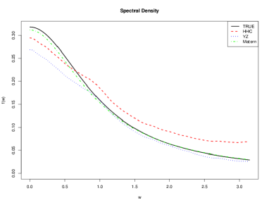
(a) Model Setup One with n=250.

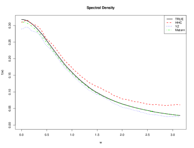
(b) Model Setup One with n=500.

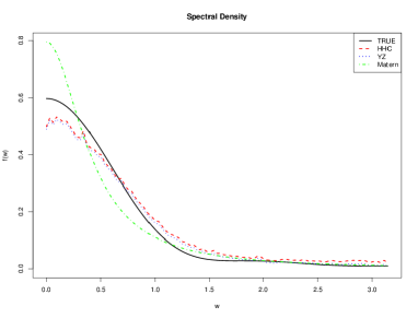
(c) Model Setup Two with n=250.

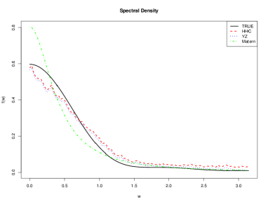
(d) Model Setup Two with n=500.

Figure 1: Spectral Density Estimation in Model Setup One and Two with n=250, 500. (a): Model Setup One with n=250; (b): Model Setup One with n=500; (c) Model Setup Two with n=250; (d) Model Setup Two with n=500. The black solid line is the true spectral density function; the red dashed line is HHC estimator; the blue dotted line is YZ estimator; and the green dashed line is the maximum likelihood estimator with a covariance model in a Matérn family..

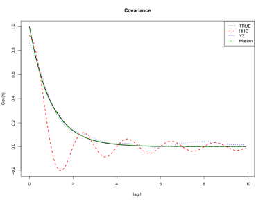
(a) Model Setup One with n=250.

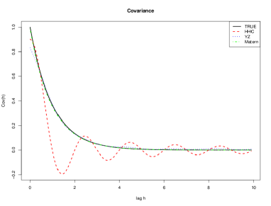
(b) Model Setup One with n=500.

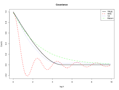
(c) Model Setup Two with n=250.

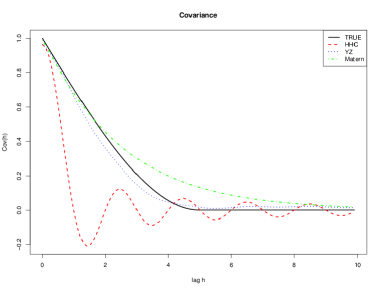
(d) Model Setup Two with n=500.

Figure 2: Covariance Function Estimation in Model Setup One and Two with n=250, 500. (a): Model Setup One with n=250; (b): Model Setup One with n=500; (c) Model Setup Two with n=250; (d) Model Setup Two with n=500. The black solid line is the true spectral density function; the red dashed line is HHC estimator; the blue dotted line is YZ estimator; and the green dashed line is the maximum likelihood estimator with a covariance model in a Matérn family..

Table 1: Monte Carlo Simulation Result in Model Setup One and Two. In Model Setup One, the data generating model uses Matérn Covariance. In Model Setup Two, the data generating model uses Spherical Covariance. The estimation methods include (1)HHC: the smoothing spline approach as proposed in HHC11b; (2)YZ: the proposed estimator in the paper (initial of the authors); (3) Matérn : maximum likelihood approach with a covariance model in a Matérn family. The evaluation measures include (A) ISE(f):the integrated squared error of spectral density function estimator; (B) ISE(C): the integrated squared error of covariance function estimator; (C) mIPE: the Monte Carlo median of the increase in prediction error .

			Model Setup One				Model Setup Two
			with Matérn Covariance				with Spherical Covariance
n			$ISE(f)$	$ISE(C)$	$mIPE$		$ISE(f)$	$ISE(C)$	$mIPE$
	HHC		0.0090	0.1201	56.650		0.0312	0.6880	89.480
250	YZ		0.0097	0.0501	0.1633		0.0214	0.0875	1.2081
	Matérn		0.0055	0.0226	0.1401		0.0388	0.1034	1.3944
	HHC		0.0078	0.0836	3.0119		0.0188	0.7420	13.5128
500	YZ		0.0075	0.0558	0.1133		0.0164	0.0866	0.9217
	Matérn		0.0039	0.0205	0.0550		0.0244	0.0967	0.9781
	HHC		0.0035	0.0827	1.3007		0.0103	0.7333	10.046
1000	YZ		0.0027	0.0242	0.1104		0.0091	0.0590	0.8001
	Matérn		0.0019	0.0118	1.5e-4		0.0245	0.0799	0.9123

5 Discussion Remarks

In this paper we proposed a semi-parametric method to estimate spectral densities of isotropic Gaussian processes observed at irregular locations on $\mathbb{R}^{1}$. The methodology can be adapted for spectral density estimation of spatial processes that are stationary or intrinsic random processes on $\mathbb{R}^{d}$ with $d>1$. Such extension will be addressed in a separate paper.

The proposed estimator is in a closed form, so it does not require heavy numerical computation. Therefore it is feasible for large-scale spatial data. It also allows us to derive asymptotic bounds for the bias and variance of the proposed estimator, and to prove the estimator is consistent in theory.

Our method builds on HHC estimator in HHC11b. The difference is that we additionally estimate the spectral density at high frequencies which has been ignored in HHC11b. The rationale is that the tail properties of the spectral function play a fundamental role in the prediction. Our simulation study shows that the proposed estimator outperforms HHC estimator in Kriging prediction.

This semi-parametric method allows modeling the spectral density at low frequencies, and therefore it is more flexible than the fully parametric approach.

Appendix A Proof of Theorem 1

Since in the estimator (13), we have involved log of the empirical variogram estimate instead of the empirical variogram estimate itself, we first derive the moment property for $\log u_{m}$. By Taylor expansion technique,

$$E\left[\log u_{m}\right] \simeq \log E\left[u_{m}\right]-\frac{1}{2\left(E\left[u_{m}\right]\right)^{2}}E\left[\left(u_{m}-E\left[u_{m}\right]\right)^{2}\right]$$

$$= \alpha_{0}\log h_{m}+O\left(h_{m}^{\alpha_{1}}\right)+O\left(N_{m}^{-1}\right).$$

The second equality follows from (12) and the approximated variance of $u_{m}$. Combining $M$ individual terms,

$$E\left[\sum_{m=1}^{M}\log u_{m}\left(\log h_{m}-\overline{\log h}_{M}\right)\right]$$

$$\simeq \sum_{m=1}^{M}\left\{\alpha_{0}\log h_{m}+O(h_{m}^{\alpha_{1}})+O\left(N_{m}^{-1}\right)\right\}\left(\log h_{m}-\overline{\log h}_{M}\right).$$

Therefore, the square bias term can be derived:

$$\left\{E\left(\hat{\alpha}_{0}-\alpha_{0}\right)\right\}^{2} = [\frac{\sum_{m=1}^{M}\left\{O(h_{m}^{\alpha_{1}})+O\left(N_{m}^{-1}\right)\right\}\left(\log h_{m}-\overline{\log h}_{M}\right)}{\sum_{m=1}^{M}\left(\log h_{m}-\overline{\log h}_{M}\right)^{2}}]^{2}$$

$$= O\left(N^{-2b\alpha_{1}}(\log N)^{-2}\right)+O\left(N^{2b^{\prime}-2}(\log N)^{-2}\right)$$

$$= O\left(\max(N^{-2b\alpha_{1}},N^{2b^{\prime}-2})(\log N)^{-2}\right),$$

and the variance term is

$$Var\left[\hat{\alpha}_{0}\right] = \frac{Var\left[\sum_{m=1}^{M}\log u_{m}\left(\log h_{m}-\overline{\log h}_{M}\right)\right]}{\left\{\sum_{m=1}^{M}\left(\log h_{m}-\overline{\log h}_{M}\right)^{2}\right\}^{2}}$$

$$= \frac{\sum_{m=1}^{M}\sum_{l=1}^{M}Cov\left(\log u_{m},\log u_{l}\right)\left(\log h_{m}-\overline{\log h}_{M}\right)\left(\log h_{l}-\overline{\log h}_{M}\right)}{\left\{\sum_{m=1}^{M}\left(\log h_{m}-\overline{\log h}_{M}\right)^{2}\right\}^{2}}$$

$$\simeq \frac{\sum_{m=1}^{M}\sum_{l=1}^{M}\frac{Cov\left(u_{m},u_{l}\right)}{E\left(u_{m}\right)E\left(u_{l}\right)}\left(\log h_{m}-\overline{\log h}_{M}\right)\left(\log h_{l}-\overline{\log h}_{M}\right)}{\left\{\sum_{m=1}^{M}\left(\log h_{m}-\overline{\log h}_{M}\right)^{2}\right\}^{2}}$$

$$\leq \frac{\sum_{m=1}^{M}\sum_{l=1}^{M}\frac{\sqrt{Var\left(u_{m}\right)Var\left(u_{l}\right)}}{E\left(u_{m}\right)E\left(u_{l}\right)}|(\log h_{m}-\overline{\log h}_{M})(\log h_{l}-\overline{\log h}_{M})|}{\left\{\sum_{m=1}^{M}\left(\log h_{m}-\overline{\log h}_{M}\right)^{2}\right\}^{2}}$$

$$\simeq \frac{\sum_{m=1}^{M}\sum_{l=1}^{M}\frac{2\gamma(h_{m})\gamma(h_{l})}{\sqrt{|N_{m}||N_{l}|}E\left(u_{m}\right)E\left(u_{l}\right)}|(\log h_{m}-\overline{\log h}_{M})(\log h_{l}-\overline{\log h}_{M})|}{\left\{\sum_{m=1}^{M}\left(\log h_{m}-\overline{\log h}_{M}\right)^{2}\right\}^{2}}$$

$$= O\left(N^{b^{\prime}-1}\left(\log N\right)^{-2}\right).$$

Combining the squared bias term and the variance term, we have

$$E\left[\left(\hat{\alpha}_{0}-\alpha_{0}\right)^{2}\right]=O\left(\max\left(N^{-2b\alpha_{1}},N^{b^{\prime}-1}\right)(\log N)^{-2}\right).$$

Appendix B Proof of Theorem 2

Write the spectral density based on the gridized data as

$$f_{\Delta}(\omega)=\frac{1}{\omega_{c}}\sum_{k=-\infty}^{\infty}\cos(\frac{k\pi\omega}{\omega_{c}})C(\frac{k\pi}{\omega_{c}}),$$

for $\omega\in[0,\omega_{c}]$. From the aliasing problem, we also have $f_{\Delta}(\omega)=\sum_{j=-\infty}^{\infty}f(\omega+2j\omega_{c})$.

Firstly, we consider the bias of the spectral density estimator at the cutoff value $\omega_{c}$. From (9),

$$|E[\hat{f}_{\Delta,\lambda}(\omega_{c})]-f_{\Delta}(\omega_{c})|$$ (23)

$$= \frac{1}{\omega_{c}}|C(0)+2\sum_{k=1}^{K}\frac{n_{k}}{n_{k}+k^{2}\lambda}\cos(k\pi)E[S_{k}]-\sum_{k=-\infty}^{\infty}\cos(k\pi)C(\frac{k\pi}{\omega_{c}})|.$$

By Taylor expansion technique,

$$E[S_{k}] = \sum_{(t_{i},t_{j})\in L_{k}}E[X(s_{i})X(s_{j})]$$

$$= \sum_{(t_{i},t_{j})\in L_{k}}C(|s_{i}-s_{j}|)$$

$$= \sum_{(t_{i},t_{j})\in L_{k}}\{C(\frac{k\pi}{\omega_{c}})+C^{(1)}(\xi_{i,j,k})(|s_{i}-s_{j}|-\frac{k\pi}{\omega_{c}})\}$$

where $\xi_{i,j,k}\in k\pi/\omega_{c}\pm\pi/\omega_{c}$. Therefore (23) becomes

$$|E[\hat{f}_{\Delta,\lambda}(\omega_{c})]-f_{\Delta}(\omega_{c})|$$ (24)

$$= \frac{1}{\omega_{c}}|C(0)+2\sum_{k=1}^{K}\frac{n_{k}}{n_{k}+k^{2}\lambda}\cos(k\pi)C(\frac{k\pi}{\omega_{c}})-\sum_{k=-\infty}^{\infty}\cos(k\pi)C(\frac{k\pi}{\omega_{c}})$$

$$+2\sum_{k=1}^{K}\frac{n_{k}}{n_{k}+k^{2}\lambda}\sum_{(t_{i},t_{j})\in L_{k}}C^{(1)}(\xi_{i,j,k})(|s_{i}-s_{j}|-\frac{k\pi}{\omega_{c}})|$$

$$\leq \frac{2}{\omega_{c}}\{\sum_{k=1}^{K}\frac{k^{2}\lambda}{n_{k}+k^{2}\lambda}|C(\frac{k\pi}{\omega_{c}})|+\sum_{k=K+1}^{\infty}|C(\frac{k\pi}{\omega_{c}})|$$

$$+ \sum_{k=1}^{K}\frac{n_{k}}{n_{k}+k^{2}\lambda}\sum_{(t_{i},t_{j})\in L_{k}}|C^{(1)}(\xi_{i,j,k})(|s_{i}-s_{j}|-\frac{k\pi}{\omega_{c}})|\}$$

$$\leq C\left\{\frac{\lambda\omega_{c}^{2}}{N}+\left(\frac{\omega_{c}}{N}\right)^{\alpha}\right\}+C\left\{\frac{2}{\omega_{c}}\sum_{k=K+1}^{\infty}\left(\frac{k\pi}{\omega_{c}}\right)^{-\alpha-1}\right\}+C\left\{\frac{1}{\omega_{c}}\right\}$$

$$\leq C\left\{\frac{\lambda\omega_{c}^{2}}{N}+\left(\frac{\omega_{c}}{N}\right)^{\alpha}+\left(\frac{\omega_{c}}{K}\right)^{\alpha}+\frac{1}{\omega_{c}}\right\}$$

$$\leq C\left\{\frac{\lambda\omega_{c}^{2}}{N}+\left(\frac{\omega_{c}}{N}\right)^{\alpha}+\frac{1}{\omega_{c}}\right\},$$

where the third term in the second last inequality follows from the third condition and

$$\sum_{k=1}^{K}\frac{n_{k}}{n_{k}+k^{2}\lambda}\sum_{(t_{i},t_{j})\in L_{k}}|C^{(1)}(\xi_{i,j,k})(|s_{i}-s_{j}|-\frac{k\pi}{\omega_{c}})|$$

$$\leq \frac{C}{\omega_{c}}\sum_{k=1}^{K}\frac{n_{k}}{n_{k}+k^{2}\lambda}Q(\frac{k\pi}{\omega_{c}})$$

$$= \frac{C}{\omega_{c}}\left\{\sum_{k<\omega_{C}}\frac{n_{k}}{n_{k}+k^{2}\lambda}Q(\frac{k\pi}{\omega_{c}})+\sum_{k\geq\omega_{C}}\frac{n_{k}}{n_{k}+k^{2}\lambda}Q(\frac{k\pi}{\omega_{c}})\right\}$$

$$\leq O(1).$$

So the bias of $\hat{\phi}$, which is the estimator of spectral density at the cut-off value can be derived as

$$|E[\hat{\phi}]-\phi| = |\frac{E\left[\hat{f}_{\Delta,\lambda}(\omega_{c})\right]}{\sum_{j=-\infty}^{\infty}|1+2j|^{-\gamma}}-f(\omega_{c})+O\left(\frac{\max(N^{-b\alpha_{1}},N^{b^{\prime}-1})}{\log N}\right)|$$ (25)

$$= |\frac{\left\{E\left[\hat{f}_{\Delta,\lambda}(\omega_{c})\right]-f_{\Delta}(\omega_{c})\right\}+\sum_{j=-\infty}^{\infty}f((1+2j)\omega_{c})}{\sum_{j=-\infty}^{\infty}|1+2j|^{-\gamma}}-f(\omega_{c})$$

$$+O\left(\frac{\max(N^{-b\alpha_{1}},N^{b^{\prime}-1})}{\log N}\right)|$$

$$\leq C\left\{\frac{\lambda\omega_{c}^{2}}{N}+\left(\frac{\omega_{c}}{N}\right)^{\alpha}+(\frac{1}{\omega_{c}})+\frac{\max(N^{-b\alpha_{1}},N^{b^{\prime}-1})}{\log N}\right\}$$

since $E[\hat{\gamma}]=\gamma+O\left(\max\left(N^{-b\alpha_{1}},N^{b^{\prime}-1}\right)(\log N)^{-1}\right)$ from Theorem 1 and $0<\sum_{j=-\infty}^{\infty}|1+2j|^{-\gamma}<\infty$.

Finally, to derive asymptotic bound for the bias of spectral density for $\omega\in[0,\omega_{c}]$, we decompose the bias into three terms as follows,

$$|bias\left(\hat{f}(\omega)\right)| = |E\left[\hat{f}(\omega)\right]-f(\omega)|$$

$$= |\left\{E[\hat{f}_{\Delta,\lambda}(\omega)]-f_{\Delta}(\omega)\right\}+\left\{f_{\Delta}(\omega)-\sum_{j=\infty}^{\infty}f(\omega+2j\omega_{c})\right\}$$

$$+\left\{\sum_{j\neq 0}f(\omega+2j\omega_{c})-E[\hat{\phi}]\sum_{j\neq 0}\left(\frac{|\omega+2j\omega_{c}|}{\omega_{c}}\right)^{-\gamma}\right\}|$$

$$\leq U_{1}+U_{2}+U_{3},$$

where

$$U_{1} = |E[\hat{f}_{\Delta,\lambda}(\omega)]-f_{\Delta}(\omega)|$$

$$\leq C\left\{\frac{\lambda\omega_{c}^{2}}{N}+\left(\frac{\omega_{c}}{N}\right)^{\alpha}+\frac{1}{\omega_{c}}\right\},$$

by the same argument in (24), $U_{2}=f_{\Delta}(\omega)-\sum_{j=\infty}^{\infty}f(\omega+2j\omega_{c})=0,$ and by (25)

$$U_{3} =| \sum_{j\neq 0}f(\omega+2j\omega_{c})-E[\hat{\phi}]\sum_{j\neq 0}\left(\frac{|\omega+2j\omega_{c}|}{\omega_{c}}\right)^{-\gamma}|$$

$$\leq C\left\{\frac{\lambda\omega_{c}^{2}}{N}+\left(\frac{\omega_{c}}{N}\right)^{\alpha}+\frac{1}{\omega_{c}}+\frac{\max(N^{-b\alpha_{1}},N^{b^{\prime}-1})}{\log N}\right\}.$$

Thus, we have the first part result in Theorem 2,

$$|bias\left(\hat{f}(\omega)\right)| \leq C\left\{\frac{\lambda\omega_{c}^{2}}{N}+\left(\frac{\omega_{c}}{N}\right)^{\alpha}+\frac{1}{\omega_{c}}+\frac{\max(N^{-b\alpha_{1}},N^{b^{\prime}-1})}{\log N}\right\}.$$

Since the bias of the spectral density estimator for $\omega\in(\omega_{c},\infty)$ is always less than the bias at $\omega=\omega_{c}$, the above bound can be applied for $\omega\in(\omega_{c},\infty)$.

To derive asymptotic bound for the variance of $\hat{f}(\omega)$ , we first consider the variance of $\hat{f}(\omega)$ when $\gamma$ is known. Let

$$a(\omega,\gamma)=\frac{\sum_{j\neq 0}\left(\frac{|\omega+2j\omega_{c}|}{\omega_{c}}\right)^{-\gamma}}{\sum_{j=-\infty}^{\infty}|1+2j|^{-\gamma}}.$$

Write

$$var\left(\hat{f}(\omega|\gamma)\right)=\sum_{k_{1}=0}^{K}\sum_{k_{2}=0}^{K}b_{k_{1}}b_{k_{2}}cov\left(S_{k_{1}},S_{k_{2}}\right),$$

where $b_{k}=\left(\cos(k\pi\omega/\omega_{c})-a(\omega)\cos(k\pi)\right)/\left(n_{k}+2(k\pi)^{2}\lambda\right)$. Note that for all $\omega\in[0,\omega]$, $|a(\omega)|<1$, use the same derivation in HHC11b , we have

$$var\left(\hat{f}(\omega|\gamma)\right)\leq\frac{C}{\sqrt{N\lambda}}.$$

Now consider variance of $\hat{f}(\omega)=\hat{f}(\omega|\hat{\gamma})$, since by Taylor expansion,

$$\hat{f}(\omega|\hat{\gamma})=\hat{f}(\omega|\gamma)+\frac{\partial}{\partial\gamma}\hat{f}(\omega|\gamma)|_{\gamma=\gamma^{\prime}}(\hat{\gamma}-\gamma),$$

where $\gamma^{\prime}$ is between $\gamma$ and $\hat{\gamma}$. Let $V_{1}=\partial\hat{f}(\omega|\gamma)/\partial\gamma|_{\gamma=\gamma^{\prime}}=C\hat{f}_{\Delta,\lambda}(\omega_{c})$, $V_{2}=\hat{\gamma}-\gamma$, when $V_{1}$ and $V_{2}$ are normally distributed, we have

$$Var(V_{1}V_{2}) = [E(V_{1})]^{2}Var(V_{2})+[E(V_{2})]^{2}Var(V_{1})$$

$$+2E(V_{1})E(V_{2})Cov(V_{1},V_{2})+Var(V_{1})Var(V_{2})+Cov(V_{1},V_{2})^{2}$$

$$\leq O\left(N^{b^{\prime}-1}\left(\log N\right)^{-2}\right)+O\left(\max(N^{-2b\alpha_{1}},N^{2b^{\prime}-2})(\log N)^{-2}(N\lambda)^{-1/2}\right)$$

$$+O\left(\max(N^{-b\alpha_{1}},N^{b^{\prime}-1})(\log N)^{-1}N^{(b^{\prime}-1)/2}\left(\log N\right)^{-1}(N\lambda)^{-1/4}\right)$$

$$+O\left(N^{b^{\prime}-1}\left(\log N\right)^{-2}(N\lambda)^{-1/2}\right)$$

$$\leq O\left(N^{b^{\prime}-1}\left(\log N\right)^{-2}\right)$$

$$+ O\left(\max(N^{-b\alpha_{1}},N^{b^{\prime}-1})(\log N)^{-2}N^{(b^{\prime}-1)/2}(N\lambda)^{-1/4}\right)$$

$$\leq O\left(N^{b^{\prime}-1}\left(\log N\right)^{-2}\right)+O\left(N^{-b\alpha_{1}}(\log N)^{-2}N^{(b^{\prime}-1)/2}(N\lambda)^{-1/4}\right)$$

Thus

$$Var\left(\hat{f}(\omega|\hat{\gamma})\right) = Var\left(\hat{f}(\omega|\gamma)+V_{1}V_{2}\right)$$

$$= Var(\hat{f}(\omega|\gamma))+2Cov(\hat{f}(\omega|\gamma),V_{1}V_{2})+Var(V_{1}V_{2}))$$

$$\leq C\left\{\frac{1}{\sqrt{N\lambda}}+\frac{N^{b^{\prime}-1}}{(\log N)^{2}}+\frac{N^{-b\alpha_{1}}N^{(b^{\prime}-1)/2}}{(\log N)^{2}(N\lambda)^{1/4}}\right\}.$$

References

References

• [1] D. Krige, A statistical approach to some mine valuation and allied problems on the witwatersrand: By dg krige, Ph.D. thesis, University of the Witwatersrand (1951).
• [2] N. Cressie, Fitting variogram models by weighted least squares, Journal of the International Association for Mathematical Geology 17 (5) (1985) 563–586.
• [3] K. V. Mardia, R. Marshall, Maximum likelihood estimation of models for residual covariance in spatial regression, Biometrika 71 (1) (1984) 135–146.
• [4] M. L. Stein, Z. Chi, L. J. Welty, Approximating likelihoods for large spatial data sets, Journal of the Royal Statistical Society: Series B (Statistical Methodology) 66 (2) (2004) 275–296.
• [5] A. M. Yaglom, Correlation theory of stationary and related random functions, Springer, 1987.
• [6] M. Abramowitz, I. A. Stegun, et al., Handbook of mathematical functions, Vol. 1, Dover New York, 1972.
• [7] G. Wahba, Automatic smoothing of the log periodogram, Journal of the American Statistical Association 75 (369) (1980) 122–132.
• [8] K. I. BeltraTo, P. Bloomfield, Determining the bandwidth of a kernel spectrum estimate, Journal of Time Series Analysis 8 (1) (1987) 21–38.
• [9] C. M. Hurvich, Data-driven choice of a spectrum estimate: extending the applicability of cross-validation methods, Journal of the American Statistical Association 80 (392) (1985) 933–940.
• [10] C. M. Hurvich, K. I. Beltrato, Cross-validatory choice of a spectrum estimate and its connections with aic, Journal of time series analysis 11 (2) (1990) 121–137.
• [11] Y. Pawitan, F. O’sullivan, Nonparametric spectral density estimation using penalized whittle likelihood, Journal of the American Statistical Association 89 (426) (1994) 600–610.
• [12] J. Fan, E. Kreutzberger, Automatic local smoothing for spectral density estimation, Scandinavian Journal of Statistics 25 (2) (1998) 359–369.
• [13] A. Shapiro, J. Botha, Variogram fitting with a general class of conditionally nonnegative definite functions, Computational Statistics & Data Analysis 11 (1) (1991) 87–96.
• [14] M. G. Genton, D. J. Gorsich, Nonparametric variogram and covariogram estimation with fourier–bessel matrices, Computational statistics & data analysis 41 (1) (2002) 47–57.
• [15] P. Hall, N. I. Fisher, B. Hoffmann, On the nonparametric estimation of covariance functions, The Annals of Statistics (1994) 2115–2134.
• [16] P. H. Garcıa-Soidán, M. Febrero-Bande, W. González-Manteiga, Nonparametric kernel estiion of an isotropic variogram, Journal of statistical planning and inference 121 (1) (2004) 65–92.
• [17] C. Huang, T. Hsing, N. Cressie, Spectral density estimation through a regularized inverse problem.
• [18] C. Huang, T. Hsing, N. Cressie, Nonparametric estimation of the variogram and its spectrum, Biometrika 98 (4) (2011) 775–789.
• [19] M. L. Stein, Interpolation of spatial data: some theory for kriging, Springer, 1999.
• [20] H. K. Im, M. L. Stein, Z. Zhu, Semiparametric estimation of spectral density with irregular observations, Journal of the American Statistical Association 102 (478) (2007) 726–735.
• [21] M. S. Bartlett, Periodogram analysis and continuous spectra, Biometrika (1950) 1–16.
• [22] U. Grenander, M. Rosenblatt, Statistical spectral analysis of time series arising from stationary stochastic processes, The Annals of Mathematical Statistics (1953) 537–558.
• [23] E. Parzen, On consistent estimates of the spectrum of a stationary time series, The Annals of Mathematical Statistics (1957) 329–348.
• [24] G. Jenkins, Dg watts, 1968: Spectral analysis and its applications.
• [25] C. C. Taylor, S. J. Taylor, Estimating the dimension of a fractal, Journal of the Royal Statistical Society. Series B (Methodological) (1991) 353–364.
• [26] A. Constantine, P. Hall, Characterizing surface smoothness via estimation of effective fractal dimension, Journal of the Royal Statistical Society. Series B (Methodological) (1994) 97–113.
• [27] P. Hall, On the effect of measuring a self-similar process, SIAM Journal on Applied Mathematics 55 (3) (1995) 800–808.
• [28] G. Chan, P. Hall, D. Poskitt, Periodogram-based estimators of fractal properties, The Annals of Statistics (1995) 1684–1711.
• [29] J. T. Kent, A. T. Wood, Estimating the fractal dimension of a locally self-similar gaussian process by using increments, Journal of the Royal Statistical Society. Series B (Methodological) (1997) 679–699.
• [30] J. Istas, G. Lang, Quadratic variations and estimation of the local hölder index of a gaussian process, in: Annales de l’Institut Henri Poincare (B) Probability and Statistics, Vol. 33, Elsevier, 1997, pp. 407–436.
• [31] Z. Zhu, M. L. Stein, Parameter estimation for fractional brownian surfaces, Statistica Sinica 12 (3) (2002) 863–884.
• [32] P. M. Broersen, R. Bos, Estimating time-series models from irregularly spaced data, Instrumentation and Measurement, IEEE Transactions on 55 (4) (2006) 1124–1131.
• [33] L. Eyer, P. Bartholdi, Variable stars: which nyquist frequency?, arXiv preprint astro-ph/9808176.
• [34] W. H. Press, W. Vetterling, S. A. Teukolsky, B. P. Flannery, E. Greenwell Yanik, Numerical recipes in fortran–the art of scientific computing, SIAM Review 36 (1) (1994) 149–149.
• [35] M. Villalobos, G. Wahba, Inequality-constrained multivariate smoothing splines with application to the estimation of posterior probabilities, Journal of the American Statistical Association 82 (397) (1987) 239–248.
• [36] N. Cressie, Statistics for spatial data, Terra Nova 4 (5) (1992) 613–617.
• [37] M. B. Priestley, Spectral analysis and time series.
• [38] U. Grenander, M. Rosenblatt, Statistical analysis of stationary time series.
• [39] K. Yu, J. Mateu, E. Porcu, A kernel-based method for nonparametric estimation of variograms, Statistica Neerlandica 61 (2) (2007) 173–197.