Taxicab Correspondence Analysis of Sparse Two-Way Contingency Tables;

Abstract

Visualization and interpretation of contingency tables by correspondence analysis (CA), as developed by Benzécri, have a rich structure based on Euclidean geometry. However, it is a well established fact that, often CA is very sensitive to sparse contingency tables, where we characterize sparsity as the existence of relatively high-valued counts, rare observations and zero-block structure. Our main aim in this paper is to highlight the above mentioned three interrelated points in two ways: First, we propose a 7-number summary of sparsity based on the minimal size of an equivalent contingency table, where the invariance property of CA and TCA (a L₁ variant of CA named taxicab) is used to construct the equivalence class of contingency tables; second, we compare the maps obtained by CA and TCA to explore under what conditions the CA and TCA maps produce similar, somewhat similar or dissimilar maps. Examples are provided.

Key words: Sparse contingency tables; correspondence analysis; taxicab correspondence analysis; interpretable maps; 7-number summary of sparsity.

1 Introduction

Correspondence analysis (CA), developed by Benzécri (1973) since 1960s, as a statistical method for different kinds of data sets, in particular for contingency tables, is embedded both in theory and in practice. The theory is based on the chi-square distance between the profiles; parallel to this beautiful theory, the practice is entrenched in the joint interpretation of the graphical displays based on the Euclidean geometry. Seeing this extreme fondness of the use and interpretation of the maps by the users of CA, Nishisato (1998) suggested the replacement of the adage “seeing is believing“ with “graphing is believing“ and stressed the importance of interpretable graphs. Additionally, we recall the often cited quip “a picture is worth a thousand words“, and via geometric interpretation of maps CA offers much to the analysis of complex multivariate data sets. So the philosophical question asked by Schlick (2000, part 5) ”Theory and Observation: Is seeing believing ?” is quite relevant here in the context of data analysis by CA.

It is well known that, CA is very sensitive to some particularities of a data set; further, how to identify and handle these is an open unresolved problem. Here, we enumerate three under the umbrella of sparse contingency tables: rare observations, zero-block structure and relatively high-valued cells. Rao (1995), among others, stressed the influence of rare observations (rows or columns that have relatively small marginal weights compared to others) and proposed an alternative to CA based on Hellinger distance ( a square-root transformation of counts). Greenacre (2013) refuted Rao’s assertion and argued that rare observations do not have an exaggerated influence in CA. Earlier Nowak and Bar-Hen (2005) developed a criterion based on the influence function to identify influential rare observations; and they arrived at the same conclusion as Greenacre in their analysis of a $207\times 15$ abundance data in ecology; however they observed that ”influential species are rare species that are concentrated in few plots”. A similar observation is found in Greenacre (2013) ”there is one exceptional situation where rare species would have a strong role in the solution, namely when a species is observed in a single sampling site and no or very few other species are observed there”. We describe this particular situation as the existence of a large zero-block structure. Often few relatively high-valued cells, including outlier counts, have detrimental effect on the CA outputs by emphasizing some aspects of the data, even though apparently the interpretation of the CA maps seems meaningful to the researchers. Our main aim in this paper is to highlight the above mentioned three points by comparing the maps obtained by CA with the maps obtained by taxicab correspondence analysis (TCA), where TCA is a L₁ variant of CA; and to explore under what conditions the CA and TCA maps produce similar, somewhat similar or dissimilar maps. Our main conclusion is that: First, CA and TCA maps enrich each other; second, for sparse contingency tables, there is a positive probability that CA and TCA maps are partially similar or dissimalar. To do this we organize the paper in six sections.

In section 2, we attempt to quantify the notion of sparsity in contingency tables by a 7-number summary based on the minimal size of an equivalent contingency table, where the invariance property of CA and TCA is used to construct the equivalence class of contingency tables. In section 3, we present a brief mathematical comparison of CA and TCA; in section 4 we present an empirical comparison using ten data sets; in section 5 we consider sparsest contingency tables; and we conclude in section 6.

The theory of CA can be found, among others, in Benzécri (1973, 1992), Greenacre (1984), Gifi (1990), Le Roux and Rouanet (2004), Murtagh (2005), and Nishisato (2007); the recent book, authored by Beh and Lombardi (2014), presents a panoramic review of CA and related methods. Since 2006, Choulakian and coauthors have studied mathematical properties of TCA applied to many kinds of non-negative data; in particular, TCA of contingency tables and their comparison with CA are studied in the following papers: Choulakian (2006), Choulakian et al. (2006), Choulakian (2008), and Choulakian, Simonetti and Gia (2014).

2 7-number summary of sparsity in contingency tables

Let ${\bf N=(}n_{ij})$ be a contingency table cross-classifying two nominal variables with $I$ rows and $J$ columns, where for $i=1,...,I$ and $j=1,...,J,$ $n_{ij}$ represents the frequency of statistical units having the $i$th category of the row variable and the $j$th category of the column variable. Thus, $n=\sum_{i=1}^{I}\sum_{j=1}^{J}n_{ij}$ represents the sample size. In the statistical literature, generally we see that the degree of sparsity of N are based on the following two quantities

$$ave({\bf N})=\frac{\sum_{i=1}^{I}\sum_{j=1}^{J}n_{ij}}{IJ},$$

the average value of counts; and

$$\%(0\in{\bf N})=\frac{\sum_{i=1}^{I}\sum_{j=1}^{J}1_{n_{ij}=0}}{IJ}100,$$

the percentage value of zero counts, where $1_{n_{ij}=0}$ is the indicator function: $1_{n_{ij}=0}=1$ for $n_{ij}=0$ and $1_{n_{ij}\neq 0}=0$ for $n_{ij}\geq 1.$

According to Agresti and Yang (1987), ${\bf N}$ is sparse if $ave({\bf N})$ is small such that the chi-squared approximations of the goodness-of-fit statistics are inaccurate. Radavicius and Samusenko (2012) characterize ${\bf N}$ as very sparse if the sample size ($n$) is less than the number of cells ($IJ$), that is, $ave({\bf N})<1$. Greenacre (2013) uses $\%(0\in{\bf N})$ as an index of sparsity.

Another qualitative definition of sparsity is used in the Ph.D thesis of Kraus (2012), based on Agresti (2002, p.391) ”contingency tables having small cell counts are said to be sparse”. A quantification of this definition will be given in subsection 2.3.

As we stated in the introduction, our concept of sparseness is broader, it also includes relatively large valued counts; to quantify this aspect of sparseness we consider the batch of nonzero counts of ${\bf N}$, and following Tukey (1977, ch.2 or p.80), we summarize them by the 5-number summary,

$$MH1=(min,Q1,Median,Q3,max);$$

where, $min$ represents the lowest value in the batch of the positive counts, $max$ the highest value, and, $Q1$, $Median$ and $Q3$ are the three quartiles ($Q1$ and $Q3$ are the two hinges in Tukey’s terminology). Thus, from the 7-number summary ($ave({\bf X}),\%(0\in{\bf X}),MH1),$ one gets an idea on the degree of sparsity concerning its different, but complementary, aspects in a contingency table ${\bf X}$.

2.1 Equivalence class of an observed contingency table

An important property of CA and TCA is that columns or rows with identical profiles (conditional probabilities) receive identical factor scores. The factor scores are used in the graphical displays. Moreover, merging of identical profiles does not change the results of the data analysis: This is named the principle of equivalent partitioning by Nishisato (1984); it includes the famous invariance property named principle of distributional equivalence, on which Benzécri (1973) developed CA. Formally, Nishisato’s principle of equivalent partitioning is based on the following

Definition 1: Let ${\bf N}$ be a contingency table of size $I\times J$, ${\bf x=(}x_{k})$ and ${\bf y=(}y_{k})$ are two rows or two columns of ${\bf N}$ such that they are proportional

$$\frac{{\bf x}}{\sum x_{i}}=\frac{{\bf y}}{{\bf\sum}y_{i}}\text{{\bf\ \ \ \ }or{\bf\ \ \ }}{\bf(\sum}y_{i}){\bf x=\ (}\sum x_{i}){\bf y}.$$

We construct a new contingency table, $N_{reduced}$, by replacing the two elements ${\bf x}$ and ${\bf y}$ in ${\bf N}$ by one element ${\bf x}+{\bf y}$, and keeping all the other columns and rows of ${\bf N}$ the same in $N_{reduced}$. Then we say that the contingency tables ${\bf N}$ and $N_{reduced}$ are equivalent, and we write ${\bf N}\sim N_{reduced}$.
Thus the equivalence class of contingency tables of ${\bf N}$ is given by

$$\Omega({\bf N)=}\left\{{\bf X}:{\bf X}\sim{\bf N}\right\}.$$

Given that, $\Omega({\bf N)}$ contains infinite number of contingency tables equivalent to a given ${\bf N}$, we define its representative element by the unique contingency table ${\bf M}$ of minimal size; that is, among all elements of $\Omega({\bf N)}$, ${\bf M}$ has minimum number of rows and columns. We can easily deduce the following inequalities: $ave({\bf N})\leq ave({\bf M})$ and $\max({\bf N})\leq\max({\bf M}).$

2.2 Artificial example and extreme sparsity

The following contrived example illustrates the idea. Let

$${\bf N}=\left(\begin{array}[]{cccc}1&2&0&0\\ 2&4&0&0\\ 0&0&1&2\\ 3&6&0&0\end{array}\right)$$

be a two-way contingency table of size $4\times 4$. Its 7-number summary of sparsity is

$$(ave({\bf N})=1.3125,\ \%(0\in{\bf N})=50,MH1=(1,\ 1.5,\ 2,\ 3.5,\ 6)).$$

We note that the first, second and fourth rows of ${\bf N}$ are proportional to each other, so they can be lumped together into one row, and we obtain the equivalent contingency table

$${\bf N}_{1}=\left(\begin{array}[]{cccc}6&12&0&0\\ 0&0&1&2\end{array}\right)$$

of size $2\times 4$; its 7-number summary of sparsity is $(2.6250,\ 50,\ (1,\ 1.5,\ 4,\ 9,\ 12))$. Similarly, we see that the third and fourth columns of ${\bf N}_{1}$ are proportional, so they can be added together, and we obtain equivalent contingency table

$${\bf N}_{2}=\left(\begin{array}[]{ccc}6&12&0\\ 0&0&3\end{array}\right)$$

of size $2\times 3$. Similarly, we see that the first and second columns of ${\bf N}_{2}$ are proportional, so they can be added together, and we obtain the unique representative equivalent contingency table

$${\bf M}=\left(\begin{array}[]{cc}18&0\\ 0&3\end{array}\right)$$

of minimal size $2\times 2.$ The four contingency tables ${\bf N}$, ${\bf N}_{1},$ ${\bf N}_{2}$ and ${\bf M}$ are equivalent, because they belong to $\Omega({\bf N):}$ CA and TCA of ${\bf N}$, ${\bf N}_{1},$ ${\bf N}_{2}$ and ${\bf M}$ produce identical maps, because they have identical geometries within the mathematical framework of CA and TCA. However, we have four different 7-number summaries of the sparsity: we consider the one obtained from ${\bf M}$ the most representative.

We note that M is a diagonal contingency table and sparsest (most sparse), based on the following lemma, whose proof is given in the appendix.

Lemma 1: $\%(0\in{\bf M})\leq 100(1-\frac{1}{\min(I,J)}).\vskip 12.0pt plus 4.0pt minus 4.0pt$

Definition 2: A contingency table is named sparsest if $\%(0\in{\bf M})=100(1-\frac{1}{\min(I,J)}),$ and extremely sparse if $\%(0\in{\bf M})$ is very near to $100(1-\frac{1}{\min(I,J)}).$

2.3 Examples of sparse contingency data sets

Table 1 enumerates ten contingency tables and their 7-number summaries calculated on ${\bf N}$ and on ${\bf M}$. Sections 4 and 5 provide further references to these data sets. The first data set is not sparse. For the last nine of them, which are considered to be sparse, we note that:

$$Q1\leq 2\ \ \ \ \ \text{and\ \ \ \ \ }Median\leq 5,$$

which is another quantification of sparsity describing ”contingency tables having small cell counts are said to be sparse”. Furthermore, comparison of $Q3$ and $max$ values highlights very long tails for sparse contingency tables, which represents the existence of relatively high-valued counts. Concerning the equivalent tables ${\bf N}$ and ${\bf M}$, we see noticeable changes in the 7-number summaries for the two data sets 6 (Barents) and 10 (Synoptic Gospels): these two contingency tables ${\bf N}$ and ${\bf M}$ are extremely tall: the number of columns is much smaller than the number of rows; so the merging of rows essentially happened for rows having very small marginal counts of 1 or 2. For these two data sets, ${\bf M}$ can be put in the following form

$${\bf M}=\left(\begin{array}[]{c}{\bf M}_{1}\\ {\bf D}\end{array}\right),$$

where ${\bf D}$ is a square diagonal matrix.

We classify the data sets in Table 1 into three large groups according to our concept of sparsity:

Non sparse tables: Data set 1 (TV programs) belongs to this group.

Extremely sparse tables: Data set 3 (Texel) belongs to this group. Note that $\%(0\in{\bf M})=96.3\%$ is very near to $100(1-1/220)=99.5455,$ the upper bound provided in Lemma 1.

Sparse tables: the remaining eight data sets belong to this group.

It is interesting to note that for Data set 10 (Synoptic Gospels): The upper bound in Lemma 1, $100(1-1/7)=85.7143$, is quite near to $\%(0\in{\bf N})=78.2\%$, but quite far from $\%(0\in{\bf M})=45\%.\$For this reason, we characterized it as sparse and not extremely sparse.

Table 1: 7-number summary of sparsity of ten two-way contingency tables.
	size	ave	%(0)	MH1					map
									similarity
1) TV									yes
programs
N=M	$13\times 7$	55.81	0%	(3	15	40	86	271)
2) Rodents									no
N	$28\times 9$	3.96	66.7%	(1	2	5	12.3	78)
M	$21\times 9$	5.3	58.7%	(1	2	4.5	14	78)
3) Texel									no
N	$285\times 220$	0.26	96.6%	(1	1	1	4.8	97)
M	$266\times 220$	0.28	96.3%	(1	1	1	7	97)
4) Macro									partial
N	$189\times 40$	6.1	84.8%	(1	2	3	14	1848)
M	$161\times 40$	7.47	81.9%	(1	2	3	14	1848)
5) Benthos									partial
N=M	$92\times 13$	8.02	39%	(1	1	3	8	992)
6) Barents									partial
N	$446\times 10$	2.91	78.4%	(1	1	2	8	798)
M	$221\times 10$	5.87	67.5%	(1	1	3	10	903)
7) Seashore									partial
N	$126\times 68$	0.14	88%	(1	1	1	1	5)
M	$106\times 65$	0.17	86.4%	(1	1	1	1	12)
8) Punta									no
Milazzese
N=M	$31\times 19$	0.83	58.1%	(1	1	1	2	12)
9) Iversfjord									no
N=M	$37\times 14$	2.643	60%	(1	1	2	6	64)
10) Synoptic									no
Gospels
N	$7097\times 7$	0.39	78.2%	(1	1	1	2	79)
M	$796\times 7$	3.59	45%	(1	1	2	4	2740)

3 Correspondence analysis and taxicab correspondence analysis: an overview

Let ${\bf P=N/}n=(p_{ij})$ be the associated correspondence matrix of N. We define as usual $p_{i\ast}=\sum_{j=1}^{J}p_{ij}$ , $p_{\ast j}=\sum_{i=1}^{I}p_{ij},$ the vector ${\bf r=(}p_{i\ast})\in\mathbf{R}^{I},$ the vector ${\bf c=(}p_{\ast j})\in\bf{R}^{J}$, and ${\bf D}_{r}=Diag({\bf r})$ the diagonal matrix having diagonal elements $p_{i\ast},$ and similarly ${\bf D}_{c}=Diag({\bf c}).$ We suppose that ${\bf D}_{r}$ and ${\bf D}_{c}$ are positive definite metric matrices of size $I\times I$ and $J\times J$, respectively; this means that the diagonal elements of ${\bf D}_{r}$ and ${\bf D}_{c}$ are strictly positive. Let $k=rank({\bf R}_{0}{\bf),}$ where

$${\bf R}_{0}=({\bf P}-{\bf rc}^{\top})$$

is the residual matrix with respect to the independence model. CA and TCA can be considered as principal components analysis for categorical data, where ${\bf P}$ or ${\bf R}_{0}$ is decomposed into a sum of bilinear terms shown in equation (1). Equation (1) is named the data reconstruction formula, and it is obtained by generalized singular value decomposition and its taxicab version with respect to the metric matrices ${\bf D}_{r}$ and ${\bf D}_{c}$, see in particular Choulakian, Simonetti and Gia (2014):

$${\bf P}={\bf D}_{r}({\bf 1}_{I}{\bf 1}_{J}^{{}^{\top}}+\sum_{\alpha=1}^{k}{\bf f}_{\alpha}{\bf g}_{\alpha}^{{}^{\top}}/\sigma_{\alpha}){\bf D}_{c},$$

or elementwise

$$p_{ij}=p_{i\ast}p_{\ast j}\left[1+\sum_{\alpha=1}^{k}f_{\alpha}(i)g_{\alpha}(j)/\sigma_{\alpha}\right],$$ (1)

where ${\bf f}_{\alpha}$ and ${\bf g}_{\alpha}$ represent the principal coordinate scores of rows and columns, and $\sigma_{\alpha}$ is the associated dispersion measure for  $\alpha=1,...,k.$ Note that in both methods ${\bf f}_{\alpha}$ and ${\bf g}_{\alpha}$ are ${\bf D}_{r}$ and ${\bf D}_{c}$ centered respectively; that is

$${\bf f}_{\alpha}^{{}^{\top}}{\bf D}_{r}{\bf 1}_{I} = {\bf g}_{\alpha}^{{}^{\top}}{\bf D}_{c}{\bf 1}_{J}$$ (2)

$$= 0,$$

where ${\bf 1}_{I}$ is a column vector of ones of size $I$.

In CA, ${\bf f}_{\alpha}$ and ${\bf g}_{\alpha}$ satisfy

$${\bf f}_{\alpha}^{{}^{\top}}{\bf D}_{r}{\bf f}_{\alpha}={\bf g}_{\alpha}^{{}^{\top}}{\bf D}_{c}{\bf g}_{\alpha}=\sigma_{\alpha}^{2}\text{ \ \ for\ \ }\alpha=1,...,k,$$ (3)

$${\bf f}_{\alpha}^{{}^{\top}}{\bf D}_{r}{\bf f}_{\beta}={\bf g}_{\alpha}^{{}^{\top}}{\bf D}_{c}{\bf g}_{\beta}=0\text{ \ \ for\ \ }\alpha\neq\beta.$$ (4)

Equation (3) says that the ${\bf D}_{r}$ weighted L₂ norm of ${\bf f}_{\alpha}$ is $\sigma_{\alpha};$ likewise, equation (4) says that ${\bf f}_{\alpha}$ is ${\bf D}_{r}$ orthogonal to ${\bf f}_{\beta}$  for  $\alpha\neq\beta$. In CA the standard coordinate scores are ${\bf f}_{\alpha}/\sigma_{\alpha}$ for column profiles and ${\bf g}_{\alpha}/\sigma_{\alpha}$ for row profiles.

In TCA, ${\bf f}_{\alpha}$ and ${\bf g}_{\alpha}$ satisfy

$${\bf f}_{\alpha}^{{}^{\top}}{\bf D}_{r}sgn({\bf f)}_{\alpha}={\bf g}_{\alpha}^{{}^{\top}}{\bf D}_{c}sgn({\bf g}_{\alpha})=\sigma_{\alpha}\text{ \ \ for\ \ }\alpha=1,...,k,$$ (5)

$${\bf f}_{\alpha}^{{}^{\top}}{\bf D}_{r}sgn({\bf f}_{\beta})={\bf g}_{\alpha}^{{}^{\top}}{\bf D}_{c}sgn({\bf g)}_{\beta}=0\text{ \ \ for\ \ }\alpha>\beta.$$ (6)

where $sgn({\bf g}_{\alpha})=[sgn(g_{\alpha}(1)),...,sgn(g_{\alpha}(J)]^{{}^{\top}},$ and $sgn(g_{\alpha}(j))=1$ if $g_{\alpha}(j)>0,$ $sgn(g_{\alpha}(j))=-1$ otherwise. Equation (5) says that the ${\bf D}_{r}$ weighted $L_{1}$ norm of ${\bf f}_{\alpha}$ is $\sigma_{\alpha};$ likewise, equation (6) says that ${\bf f}_{\alpha}$ is ${\bf D}_{r}$ orthogonal to $sgn{\bf(f}_{\beta})$  for  $\alpha>\beta$.

2.1: Remarks

• a) CA of ${\bf P}$ is equivalent to CA of ${\bf R}_{0}$, with diagonal weight matrices ${\bf D}_{r}$ and ${\bf D}_{c}.$ Analogously, TCA of ${\bf P}$ is equivalent to TCA of ${\bf R}_{0},$ with diagonal weight matrices ${\bf D}_{r}$ and ${\bf D}_{c}.$

• b) In CA, the principal coordinate scores ${\bf f}_{\alpha}$ and ${\bf g}_{\alpha}$ are functions of the eigenvectors of a similarity measure between the rows or columns and more importantly the similarity measure depends on the chosen metric ${\bf D}_{r}$ and ${\bf D}_{c}.$ We describe the computation of ${\bf f}_{\alpha}$ and ${\bf g}_{\alpha}$ in four steps:

  Step 1: we calculate the matrix of Pearson residuals,

  $${\bf S}={\bf D}_{r}^{-1/2}({\bf P}-{\bf rc}^{{}^{\top}}){\bf D}_{c}^{-1/2}.$$ (7)

  Step 2: we calculate the eigenvectors ${\bf x}_{\alpha}$ via the eigen-equation,

  $${\bf S}^{{}^{\top}}{\bf Sx}_{\alpha}=\sigma_{\alpha}^{2}{\bf x}_{\alpha}\text{ \ \ \ with \ }{\bf x}_{\alpha}^{{}^{\top}}{\bf x}_{\alpha}=1,$$ (8)

  where the $(i,j)$th element of ${\bf S}^{{}^{\top}}{\bf S}$ represents a similarity measure between the two column categories $i$ and $j$.

  Step 3: we calculate ${\bf f}_{\alpha}=\sigma_{\alpha}{\bf D}_{r}^{-1/2}{\bf x}_{\alpha}.$

  Step 4: we calculate ${\bf g}_{\alpha}$ via the transition formula (22).

• c) Compared to CA, TCA stays as close as possible to the original data: It directly acts on the correspondence matrix ${\bf P}$ or ${\bf R}_{0}$ in the largest sense that the basic taxicab decomposition is independent of the metrics ${\bf D}_{r}$ and ${\bf D}_{c}$: it is simply constructed from a sum of the signed columns or rows of the residual correspondence matrix, for further details see Choulakian (2006, 2016); only the relative direction of the rows or columns is taken into account without calculating a similarity (or dissimilarity) measure between the rows or columns.

  The optimization criterion is based on the famous Grothendieck problem, see Pisier  (2012). The steps for the computation of the principal coordinate scores ${\bf f}_{\alpha}$ and ${\bf g}_{\alpha}$ are done iteratively for$\ \alpha=1,...,k:$

Step 1: we compute the principal axis

$${\bf u}_{\alpha}=\arg\max_{{\bf u\in}\left\{-1,1\right\}^{J}}||{\bf R}_{\alpha-1}{\bf u}||_{1},$$

where ${\bf R}_{0}={\bf P}-{\bf rc}^{{}^{\top}}$   and $\ {\bf R}_{\alpha}={\bf P}-{\bf rc}^{{}^{\top}}-\sum_{\beta=1}^{\alpha}{\bf D}_{r}{\bf f}_{\beta}{\bf g}_{\beta}^{{}^{\top}}{\bf D}_{c}/\sigma_{\beta}$ for  $\alpha=1,...,k$.

Step 2: we compute the principal coordinate scores ${\bf f}_{\alpha}={\bf D}_{r}^{-1}{\bf R}_{\alpha-1}{\bf u}_{\alpha}$.

Step 3: we calculate ${\bf g}_{\alpha}$ via the transition formula (15),

$${\bf g}_{\alpha}={\bf D}_{c}^{-1}{\bf R}_{\alpha-1}^{{}^{\top}}sgn({\bf f}_{\alpha})$$

.

Step 4: we update ${\bf R}_{\alpha+1}={\bf P}-{\bf rc}^{{}^{\top}}-\sum_{\beta=1}^{\alpha+1}{\bf D}_{r}{\bf f}_{\beta}{\bf g}_{\beta}^{{}^{\top}}{\bf D}_{c}/\sigma_{\beta}.$

• d) An interesting and useful property of the taxicab dispersion measures, $\sigma_{\alpha}$ for $\alpha\geq 1,$ is the following result well known in theoretical computer science, see Khot and Naor (2013):

  Lemma 2:

  $$\sigma_{\alpha} = \frac{||{\bf R}_{\alpha-1}{\bf u}||_{1}}{||{\bf u}||_{\infty}}\ \ \ \ \ \text{for \ \ \ }\alpha\geq 1$$

  $$= \max_{{\bf u\in}\left\{-1,1\right\}^{J}}||{\bf R}_{\alpha-1}{\bf u}||_{1}$$

  $$= 4\ ||{\bf R}_{\alpha-1}||_{cut},$$

  where the cut norm of the matrix ${\bf R}_{\alpha-1}$ is defined as

  $$||{\bf R}_{\alpha-1}||_{cut}=\max_{S\times T}\ |\sum_{(i,j)\in S\times T}{\bf R}_{\alpha-1}(i,j)|\text{\ \ where\ }\\ S\subseteq\left\{1,...,I\right\}$$

  $$\text{ and }T\subseteq\left\{1,...,J\right\}.$$

  We know that taxicab principal axes have values $\pm 1,$ that is,$\ {\bf u}_{\alpha}{\bf\in}\left\{-1,1\right\}^{J}$ and ${\bf v}_{\alpha}{\bf\in}\left\{-1,1\right\}^{I}$ for $\alpha\geq 1$. So we can represent ${\bf u}_{\alpha}={\bf u}_{\alpha+}+{\bf u}_{\alpha-},$ and similarly, ${\bf v}_{\alpha}={\bf v}_{\alpha+}+{\bf v}_{\alpha-}$, where

  $${\bf u}_{\alpha+} = ({\bf 1}_{J}+{\bf u}_{\alpha})/2$$

  $${\bf u}_{\alpha-} = ({\bf u}_{\alpha}-{\bf 1}_{J})/2.$$

  Lemma 2 can be named 4-quadrants balancing property, because the taxicab dispersion measure $\sigma_{\alpha}$ for $\alpha\geq 1$ is divided into 4 equal parts having the common value of the cut norm of ${\bf R}_{\alpha-1}$:

  $$\sigma_{\alpha}/4 = {\bf v}_{\alpha+}^{\prime}{\bf R}_{\alpha-1}{\bf u}_{\alpha+}$$

  $${\bf=} {\bf v}_{\alpha-}^{\prime}{\bf R}_{\alpha-1}{\bf u}_{\alpha-}$$

  $$= |{\bf v}_{\alpha-}^{\prime}{\bf R}_{\alpha-1}{\bf u}_{\alpha+}|$$

  $$= |{\bf v}_{\alpha+}^{\prime}{\bf R}_{\alpha-1}{\bf u}_{\alpha-}|.$$

  As a corollary to this fact, we have: In TCA of ${\bf P}$ both principal coordinate scores ${\bf f}_{\alpha}$ and ${\bf g}_{\alpha}$ for$\ \ \alpha=1,...,k$ satisfy the equivariability property, see Choulakian (2008b). This means that ${\bf f}_{\alpha}$ and ${\bf g}_{\alpha}$ are equally balanced in the sense that

  $$\frac{\sigma_{\alpha}}{2} = \sum_{i\in I_{\alpha+}}p_{i\ast}f_{\alpha}(i),$$ (9)

  $$= -\sum_{i\in I_{\alpha-}}p_{i\ast}f_{\alpha}(i),$$

  $$= \sum_{j\in J_{\alpha+}}p_{\ast j}g_{\alpha}(j),$$

  $$= -\sum_{j\in J_{\alpha-}}p_{\ast j}g_{\alpha}(j),$$

  where $I_{\alpha+}=\left\{i|f_{\alpha}(i)>0\right\}$, $I_{\alpha-}=\left\{i|f_{\alpha}(i)<0\right\},$ $J_{\alpha+}=\left\{j|g_{\alpha}(j)>0\right\}$ and $J_{\alpha-}=\left\{j|g_{\alpha}(j)<0\right\}.$ This easily follows from the fact that the principal coordinate scores ${\bf f}_{\alpha}$ and ${\bf g}_{\alpha}$ are ${\bf D}_{r}$ and ${\bf D}_{c}$ centered, they satisfy equation (2). An informal illustrative interpretation of the equivariability property is that TCA pulls inside potential influential observations and pushes outside points around the origin, thus providing a more balanced and robust view of data.

We note that in CA the principal coordinate scores ${\bf f}_{\alpha}$ and ${\bf g}_{\alpha}$ do not satisfy the equivariability property, because they are unequally balanced in the sense that

$$A = \sum_{i\in I_{\alpha+}}p_{i\ast}f_{\alpha}(i),$$

$$= -\sum_{i\in I_{\alpha-}}p_{i\ast}f_{\alpha}(i),$$

$$B = \sum_{j\in J_{\alpha+}}p_{\ast j}g_{\alpha}(j),$$

$$= -\sum_{j\in J_{\alpha-}}p_{\ast j}g_{\alpha}(j),$$

and in general,

$$A\neq B;$$

furthermore, $A$ and $B$ are not related to the dispersion measure $\sigma_{\alpha},$ because CA maximizes the variance of the principal coordinate scores.

• e) Given that the approach in CA and TCA is geometric, influence measure of a point (a column or a row) to the $\alpha$th factor is provided by the contribution of that point to the dispersion measure of the $\alpha$th factor in per 1000 units.

  In CA, based on (3), this corresponds to:

  $$C_{\alpha}(i)=1000\frac{p_{i\ast}f_{\alpha}^{2}(i)}{\sigma_{\alpha}^{2}}\text{ \ \ and \ \ \ }C_{\alpha}(j)=1000\frac{p_{j\ast}g_{\alpha}^{2}(j)}{\sigma_{\alpha}^{2}}\text{.}$$ (10)

  In TCA, based on (5), we have the signed contribution

  $$SC_{\alpha}(i)=1000\frac{p_{i\ast}f_{\alpha}(i)}{\sigma_{\alpha}}\text{ \ \ and \ \ \ }SC_{\alpha}(j)=1000\frac{p_{j\ast}g_{\alpha}(j)}{\sigma_{\alpha}}\text{.}$$ (11)

  It is important to note that, in CA,

  $$0<C_{\alpha}(point)<1000\text{;}$$ (12)

  while in TCA, from (9) we get,

  $$-500\leq SC_{\alpha}(point)\leq 500.$$ (13)

• f) In both methods the maps or joint displays are obtained by plotting (${\bf f}_{\alpha},{\bf f}_{\beta})$ and (${\bf g}_{\alpha},{\bf g}_{\beta})$ for $\alpha\neq\beta.$ Both CA and TCA have common residual transition formulas, see Choulakian (2006),

  $$f_{\alpha}(i)=p_{i\ast}^{-1}\sum_{j=1}^{J}R_{\alpha-1}(i,j)u_{\alpha}(j))\text{ \ \ for \ \ }\alpha=1,...,k,$$ (14)

  and

  $$g_{\alpha}(j)=p_{\ast j}^{-1}\sum_{i=1}^{I}R_{\alpha-1}(i,j)v_{\alpha}(i)\text{ \ \ for \ \ }\alpha=1,...,k,$$ (15)

  where R_α is the residual correspondence matrix, and ${\bf u}_{\alpha}$ and ${\bf v}_{\alpha}$ for   $\alpha=1,...,k$ are the normed principal axes and related to the principal coordinate scores ${\bf g}_{\alpha}$ and ${\bf f}_{\alpha}$ for   $\alpha=1,...,k$ in the following way. In both methods

  $${\bf R}_{\alpha}={\bf P}-{\bf rc}^{{}^{\top}}-\sum_{\beta=1}^{\alpha}{\bf D}_{r}{\bf f}_{\beta}{\bf g}_{\beta}^{{}^{\top}}{\bf D}_{c}/\lambda_{\beta}.$$ (16)

  In TCA

  $${\bf u}_{\alpha}=sgn({\bf g}_{\alpha})\text{ \ and \ }{\bf v}_{\alpha}=sgn({\bf f}_{\alpha})\text{ \ \ for \ \ }\alpha=1,...,k,$$ (17)

  so equations (14) and (15) become

  $$f_{\alpha}(i)=p_{i\ast}^{-1}\sum_{j=1}^{J}R_{\alpha-1}(i,j)sgn(g_{\alpha}(j))\text{ \ \ for \ \ }\alpha=1,...,k,$$ (18)

  and

  $$g_{\alpha}(j)=p_{\ast j}^{-1}\sum_{i=1}^{I}R_{\alpha-1}(i,j)sgn(f_{\alpha}(i))\text{ \ \ for \ \ }\alpha=1,...,k.$$ (19)

  Equations (18) and (19) help us to interpret the joint TCA maps in the following way: $f_{\alpha}(i),$ the coordinate of point $i$ on the $\alpha$th axis is the signed centroid of the residual correspondence matrix within the $p_{i\ast}^{-1}$ constant. Analogous interpretation applies to $g_{\alpha}(j),$ the coordinate of point $j$ on the $\alpha$th axis.

In CA

$${\bf u}_{\alpha}={\bf g}_{\alpha}/\sigma_{\alpha}\text{ \ and \ }{\bf v}_{\alpha}={\bf f}_{\alpha}/\sigma_{\alpha}\text{ \ \ for \ \ }\alpha=1,...,k.$$ (20)

The joint interpretation of column and row categories in the CA map is based on the well known transition formulas

$$f_{\alpha}(i)=\sum_{j=1}^{J}\Pr(j|i)g_{\alpha}(j)/\sigma_{\alpha}\text{ \ \ for \ \ }\alpha=1,...,k,$$ (21)

and

$$g_{\alpha}(j)=\sum_{i=1}^{I}\Pr(i|j)f_{\alpha}(i)/\sigma_{\alpha}\text{ \ \ for \ \ }\alpha=1,...,k,$$ (22)

where $\Pr(j|i)=p_{ij}/p_{i\ast},$ the conditional probability of observing $j$ given $i$. Note that (21, 22) can be obtained from (14, 15) via (3, 4, 20). In (21), the principal coordinate score $f_{\alpha}(i)$ is the weighted average (centroid) of the principal coordinate scores $g_{\alpha}(j)$ within the $\lambda_{\alpha}^{-1}$ constant. Analogous interpretation applies to $g_{\alpha}(j),$ the coordinate of point $j$ on the $\alpha$th axis.

4 Data analysis

Here we carry out CA and TCA on three data sets mentioned in Table 1, and comment on the remaining. The visual comparison of CA and TCA maps shows that we can have three distinct cases: similar maps, dissimilar maps, and partially similar maps.

4.1 TV programs data set

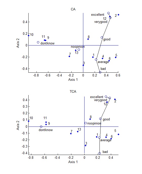
Figure 1: CA and TCA biplots of TV Programs data.

Table 2 presents a contingency table of size $13\times 7$ taken from Benzécri (1976), where a sample of 400 individuals evaluate 13 TV programs on a likert scale from 1(excellent) to 5 (bad); also two other categories of response are included noopinion on the program and dontknow the program. The data set is not sparse. Figure 1 displays CA and TCA maps, where we see that both maps are similar and produce the same interpretation. The % of explained variation for CA (resp. for TCA) of the first two dimensions are 70.7  (resp. 78%) and 21.6 (resp (16.7); with almost equivalent cumulative value of 92.4% for CA and 94.7 for TCA. The interpretation of the first two dimensions in Figure 1 will be based on two principles: principle of dichotomy and principle of gradation.

4.1.1: Interpretation of the 1st axis

We note that $C_{1}(dontknow)=700$ and $SC_{1}(dontknow)=-500$ as given at the bottom of Table 2; so the first axis represents the dichotomy between ignorance and knowledge: where the response category dontknow opposes to the 5 likert response scales; noopinion is near the origin.

4.1.2: Interpretation of the 2nd axis

The 5 Likert response categories are ordered from excellent to bad.

4.1.3: Interpretation of the TV programs

Programs 2 and 12 are considered excellent and verygood; programs 10, 11 and 9 are mostly unknown, and so on.

It is important to note that, the response category dontknow is very influential in both methods CA and TCA, and it reveals a central important feature of the data: in TCA, the category $dontknow$ contributes only to the first axis, because it attains the maximum value of its contribution, $|SC|=500$, see equation (9); but this is not the case in CA.

4.2 Rodent species abundance data set

Table 2 displays abundance data (N) of size $28\times 9$ (equivalent to M of size $21\times 9)$, where 9 species of rodents have been counted at each of 28 sites in California. For the interested reader, we identify the 9 rodents by their scientific names: rod1=Rt.rattus, rod2=Mus.musculus, rod3=Pm.californicus, rod4=Pm.eremicus, rod5=Rs.megalotis, rod6=N.fuscipes, rod7 =N.lepida,
rod8=Pg.fallax, and rod9=M.californicus. Genus abbreviations are: Rt (Rattus), Rs (Reithrodontomys), Mus (Mus), Pm (Peromyscus), Pg (Perognathus), N (Neotoma) and M (Microtus). Rattus and Mus, rodents 1 and 2, are invasive species, whereas the others are native. This data set is very interesting, because we see that it has, in particular, three specificities which characterize our concept of sparsity: rare observations, a zero-block structure and relatively high-valued cells. It is sparse based on the 7-number summary calculated in Table 1. It was proposed in 2014 as an exercise in a course on an ecology workshop in UBC in Canada; the workshop site mentions that the data set is downloaded from the web site of Quinn and Keough (2002), and it can be found at

https://www.zoology.ubc.ca/~bio501/R/workshops/workshops-
multivariate-methods/

The instructor of the course suggested the analysis of this data set by CA in two rounds:

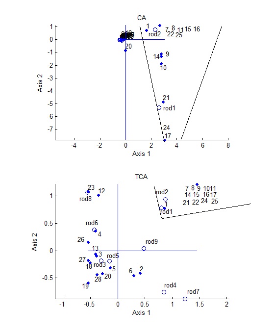
Figure 2: CA and TCA biplots of Rodents data.

In round 1 the invasive species dominate, see the CA map in Figure 2. This fact is confirmed by looking at the contibutions in Table 2, where we find $C_{1}(rod2)=750,$ so the first axis in the CA map is dominated by rodent 2; $C_{2}(rod1)=854$, so the second axis is dominated by rodent 1. The highlighted subset of sites, 7-11, 14-17, 21-22, 24-25, which are completely associated only with the invasive rodents 1 and 2, characterizes the CA solution; their total weight is $84/1002=8.38\%.$ The minimal matrix ${\bf M}$ has a zero-block structure and it can be reexpressed as

$${\bf M}=\left(\begin{array}[]{cc}{\bf M}_{1}&{\bf M}_{2}\\ {\bf M}_{3}&{\bf 0}\end{array}\right),$$

where

$${\bf M}_{3}=\left(\begin{array}[]{cc}0&59\\ 3&8\\ 1&2\\ 1&3\\ 4&0\\ 2&1\end{array}\right),$$

and the submatrix $(\begin{array}[]{cc}{\bf M}_{3}&{\bf 0}\end{array})$ represents the 13 highlighted sites. We conclude that the combination of the high count cell 59 (representing 7 rare sites), the last five rows in ${\bf M}_{3}\$(representing 6 rare sites), and the large zero-block in ${\bf M}$, created this particular CA solution.

In round 2 the instructor suggested eliminating rodents 1 and 2 and their associated sites, and carrying out a second application of CA on the reduced data set representing only the native species (the CA map is not shown).

Figure 2 displays the principal maps produced by CA and TCA, where the two invasive species and their associated sites are fenced by linear segments: they are completely different. It is evident that for this data the TCA map is much more informative than the corresponding CA map; further, one TCA map is as informative as two CA maps obtained from the two rounds.

4.2.1  Interpretation of the TCA map

Let us interpret the TCA biplot, the lower diagram in Figure 2. We note that the two invasive species are grouped and found in the first quadrant of the TCA map; further, they are associated with the 13 highlighted subset of sites that we enumerated above. The contibutions to dimensions 1 and 2 of the rodents, $SC_{1}$ and $SC_{2}$ displayed in Table 2, show that the TCA map is dominated by the four most frequent species: rodents 2, 6, 3 and 4; and each of them occupy a quadrant in the TCA map.

Let us interpret the most frequent ($freq$) species rodent 3 ( $freq=467$ out of $1002$): it dominates the third quadrant, and it is associated with site3 ($freq=36$), site5 ($freq=63$), site13 ($freq=39$), site18 ($freq=78$), site27 ($freq=29$) and site28 ($freq=10$). Rod3 is also associated with rod5, their positions are quite near on Figure 2; looking at the entries in the column of rod5, we see that its high frequency sites are site27 ($freq=10$), site18 ($freq=10$), site6 ($freq=12$), site5 ($freq=11$); further these high frequency sites 27, 18, 6 and 5 also characterize rod3. We also note that site6 is associated with both species rod3 ($freq=48$) and rod4 ($freq=35$), and its position is in between rod3 and rod4; however it is found in quadrant 3, because $(35/125)>48/467$.

4.2.2 Comparison

By comparing the first two principal dimensions in CA and TCA, we note the following two facts:

a) Rodent 2, with nonnegligeable weight (around 10%), has a very high influence on the first principal axis in CA ($C_{1}(rod2)=750);$ but it distributes its influence onto the first two principal axes in TCA ($SC_{1}(rod2)=-196$ and $SC_{2}(rod2)=-238)$.

b) Rodent 1 is a rare influential point in CA ($weight=1.4\%$ and
$C_{2}(rod1)=854$); but is no more influential in TCA
($SC_{1}(rod1)=-23$ and $SC_{2}(rod1)=-26)$.

We conclude that in Figure 2, the CA map emphasized some particular aspects of the data set; while the TCA map revealed the central abundances in Table 2.

4.3 Macro abundance data set

This macroinvertebrate sparse abundance data set of size $197\times 40$ was also considered by Greenacre (2013). Figures 3 and 4 display the CA and TCA maps: The first dimension has almost the same separation of the 40 sites, so the same interpretation; while the second dimension seems somewhat different. For this reason we labeled the map similarity partial in Table 1.

4.4 Remaining data sets

Here, we just give references for the remaining data sets listed in Table 1.

The five ecology abundance data sets numbered 3 to 7 are available in Greenacre (2013) and he discussed them in his essay.

Mallet-Gauthier and Choulakian (2015) analyse Punta Milazesse and Iverjsford abundance data in archeolgy; they reproduce the data sets, provide CA and TCA maps and their interpretations.

Choulakian et al. (2006) is the reference for the Synoptic Gospels textual count data; they provide CA and TCA maps and discuss their stability.

5 Sparsest contingency tables

Sparsest contingency tables are diagonal contingency tables, as we defined in section 2. Here, we show that CA and TCA results are completely different.

5.1 CA of sparsest contingency tables

Let ${\bf N}$ be a diagonal contingency table of size ${\it I}$, then it is well known, see for instance Benzécri (1973, p. 188) that CA of ${\bf N}$ produces $(I-1)$ dispersion measures of 1; that is, $\sigma_{\alpha}^{CA}=1$ for $\alpha=1,...,I-1.$ So, CA shows that ${\bf N}$ is composed of $I$ diagonal blocks. A similar result is known in spectral clustering as Fiedler’s theorem, see Choulakian and de Tibeiro (2013).

5.2 TCA of sparsest contingency tables

Let ${\bf P}_{{\bf N}}=diag(p_{1},...,p_{I})$ be the correspondence matrix of a diagonal contingency table ${\bf N.}$ Then we have the following easily proven result:

Corollary to Lemma 2: $\sigma_{1}^{TCA}=1$ if and only if there is a subset $S\subset\left\{1,...,I\right\}$ such that $\sum_{i\in S}p_{i}=0.5.$

proof: By Lemma 2,

$$\sigma_{1}^{TCA} = 4\ {\bf v}_{1+}^{\prime}{\bf R}_{0}{\bf u}_{1+}$$

$$= 4\ {\bf u}_{1+}^{\prime}{\bf R}_{0}{\bf u}_{1+}\text{, \ for }{\bf R}_{0}\text{ is symmetric}$$

$$= 4\ \sum_{i\in S}p_{i}(1-\sum_{i\in S}p_{i}),$$

where $S=\left\{i:{\bf u}_{1+}(i)=1\text{ for }1,...,I\right\}$, and the required result follows.

5.3 Examples

We present three exemples, two contrived and one real.

5.3.1. Example 1

Let ${\bf N=Diag(}1,\ 2,\ 3,\ 4,\ 6);$ then CA produces identical singular values $\sigma_{1}^{CA}=\sigma_{2}^{CA}=\sigma_{3}^{CA}=\sigma_{4}^{CA}=\ 1;$ while TCA produces $\sigma_{1}^{TCA}=1$ for $2+6=1+3+4,\$and the remaining dispersion measures are

$$\sigma_{\alpha}^{TCA}=0.875,\ 0.85714\ \ \$$

and$\ \ 0.18750.$

5.3.2. Example 2

Let ${\bf N=Diag(}1,\ 2,\ 3,\ 4,\ 5);$ then CA produces $\sigma_{1}^{CA}=\sigma_{2}^{CA}=\sigma_{3}^{CA}=\sigma_{4}^{CA}=\ 1;$ while TCA produces dispersion measures

$$\sigma_{\alpha}^{TCA}=0.99556,\ 0.95714,\ 0.95522\ \ \mbox{and}\ \ 0.17778.$$

5.3.3. Texel abundance data set

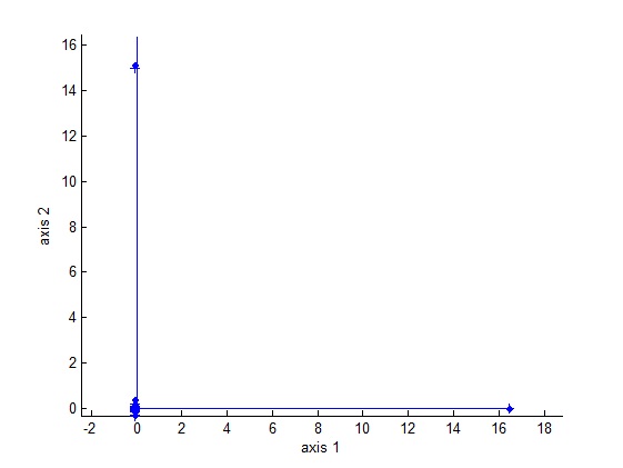
Figure 5: CA map of Texel data.

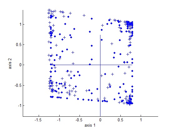
Figure 6: TCA map of Texel data.

Greenacre (2013) described this data set of size $285\times 220$ ”as large and very sparse table of vegetation abundances on a coastal sand dune area on the island of Texel, the Netherlands”. CA is of no help for the analysis of this table, because according to Greenacre CA needs as much as 71 dimensions. This is evident by looking at the sequence of CA singular values: The first five singular values are: $\sigma_{\alpha}^{CA}=\ 1,$ $0.9932,$ $0.9908,$ $0.9798$ and $0.9761;$ $\sigma_{\alpha}^{CA}=\ 1$ means that by permuting rows and columns of the data set, the data can be represented in two diagonal blocks. The corresponding TCA dispersion measures are: $\sigma_{\alpha}^{TCA}=0.8026,\ 0.7768,\ 0.7331,\ 0.7106\$and $0.7012$. Figures 5 and 6 display the CA and TCA maps, which are completely different. We leave the interpretation of the TCA map, if there is any, to the ecologists.

6 Conclusion

The fundamental aim of CA and TCA is to produce interpretable maps that reflect central contents in a data set. In this paper, first we provided a 7-number quantification of sparsity; then we showed that for sparse contingency tables CA and TCA maps can differ with positive probability, because a map produced by CA or TCA is dependent on the underlying geometry, Euclidean or Taxicab. Based on our experience, we suggest the analysis of a data set by both methods CA and TCA: Like a cubist painting where an object is painted from different angles, sometimes the views are similar, and at other times dissimilar or partially similar.

Acknowledgements.

This research has been supported by NSERC of Canada. The detailed comments of M. Greenacre and two anonymous reviewers improved the presentation of this essay significantly.

Appendix

Lemma 1: $\%(0\in{\bf N})\leq 100(1-\frac{1}{\min(I,J)}).$

The proof is very easy by considering 2 distinct cases of data sets, square $(I=J)$ and rectangular $(J>I)$.

Case 1: If ${\bf M}$ is diagonal and has exactly $I$ nonzero cells, then by permuting some rows and columns, it can be rearranged into a diagonal contingency table; thus

$$\%(0 \in {\bf M})=100(I^{2}-I)/I^{2}$$

$$= 100(1-1/I),$$

which is the upper bound. If ${\bf M}$ is a square contingency table but not diagonal, by permuting some rows and columns, it can be rearranged into a square contingency table with all diagonal cells nonzero plus some, say, $\alpha$ number of nondiagonal nonzero cells. Then it is evident that

$$\%(0 \in {\bf M})=100(I^{2}-I-\alpha)/I^{2}$$

$$\leq 100(1-1/I).$$

Case 2: ${\bf M}$ is rectangular and $(J>I)$. Then ${\bf M}=({\bf M}_{1}|{\bf M}_{2})$, where ${\bf M}_{1}$ is square with nonzero diagonal elements of size $I\times I$ and has $\alpha$ number of nondiagonal nonzero cells ; ${\bf M}_{2}$ is rectangular of size $I\times(J-I),$ such that each column of ${\bf M}_{2}$ has exactly $\beta_{i}$ nonzero cells for $i=1,...,(J-I)$ and $2\leq$ $\beta_{i}\leq I.\$Then

$$\%(0 \in {\bf M})=\frac{100\left[(IJ-I-\alpha-\sum_{i=1}^{J-I}\beta_{i})\right]}{IJ}$$

$$\leq 100(1-1/I),$$

because $\sum_{i=1}^{J-I}\beta_{i}\geq 2(J-I).\vskip 12.0pt plus 4.0pt minus 4.0pt$

References

Agresti, A. (2002). Categorical Data Analysis. New Jersey: John Wiley & Sons, 2nd edition.

Agresti, A. and Yang, M.C. (1987). An empirical investigation of some effects of sparseness in contingency tables. Computational Statistics & Data Analysis, 5, 9–21.

Beh, E. and Lombardo, R. (2014). Correspondence Analysis: Theory, Practice and New Strategies. N.Y: Wiley.

Benzécri, J.P. (1976). Sur le codage réduit d’un vecteur de description en analyse des correspondances. Les Cahiers de l’analyse des données, 1(2), 127-136.

Benzécri, J.P. (1973). L’Analyse des Données: Vol. 2: L’Analyse des Correspondances. Paris: Dunod.

Benzécri, J.P (1992). Correspondence Analysis Handbook. N.Y: Marcel Dekker.

Choulakian, V. (2006). Taxicab correspondence analysis. Psychometrika, 71, 333-345

Choulakian, V. (2008). Taxicab correspondence analysis of contingency tables with one heavyweight column. Psychometrika, 73, 309-319.

Choulakian, V., Kasparian, S., Miyake, M., Akama, H., Makoshi, N., Nakagawa, M. (2006). A statistical analysis of synoptic gospels. JADT’2006, pp. 281-288.

Choulakian, V. and de Tibeiro, J. (2013). Graph partitioning by correspondence analysis and taxicab correspondence analysis. Journal of Classification, 30, 397-427.

Choulakian, V., Allard, J. and Simonetti, B. (2013). Multiple taxicab correspondence analysis of a survey related to health services. Journal of Data Science, 11(2), 205-229.

Choulakian, V., Simonetti, B. and Gia, T.P. (2014). Some further aspects of taxicab correspondence analysis. Statistical Methods and Applications, available online.

Choulakian, V. (2016). Matrix factorizations based on induced norms.
Statistics, Optimization and Information Computing, 4, 1-14.

Gifi, A. (1990). Nonlinear Multivariate Analysis. N.Y:  Wiley.

Greenacre, M. (1984). Theory and Applications of Correspondence Analysis. Academic Press, London.

Greenacre, M. (2013). The contributions of rare objects in correspondence analysis. Ecology, 94(1), 241-249.

Khot, S. ans Naor, A. (2012). Grothendieck-type inequalities in combinatorial optimization. Communications in Pure and Applied Mathematics, 65 (7), 992-1035.

Kraus, K. (2012). On the Measurement of Model Fit for Sparse Categorical Data. Ph.D thesis, Acta Universitatis Upsaliensis, Uppsala.

Le Roux, B. and Rouanet, H. (2004). Geometric Data Analysis. From Correspondence Analysis to Structured Data Analysis. Dordrecht: Kluwer–Springer.

Mallet-Gauthier, S. and Choulakian, V. (2015). Taxicab correspondence analysis of abundance data in archeology: three case studies revisited. Archeologia e Calcolatori, 26, 77-94.

Murtagh, F. (2005). Correspondence Analysis and Data Coding with Java and R. Boca Raton, FL., Chapman & Hall/CRC.

Nishisato, S. (1984). Forced classification: A simple application of a quantification method. Psychometrika, 49(1), 25-36.

Nishisato, S. (2007). Mutidimensional nonlinear descriptive analysis. Chapman & Hall/CRC, Boca Raton.

Nishisato, S. (1998). Graphing is believing: interpretable graphs for dual scaling. In Blasius, J. and Greenacre, M. (eds.), ”Visualization of Categorical Data”, Academic Press, NY, 185-196.

Nowak, E. and Bar-Hen, A. (2005). Influence function and correspondence analysis. Journal of Statistical Planning and Inference, 134, 26-35.

Pisier, G. (2012). Grothendieck’s theorem, past and present. Bulletin of the American Mathematical Society, 49 (2), 237-323.

Quinn, G. and Keough, M. (2002). Experimental Design and Data Analysis for Biologists. Cambridge Univ. Press, Cambridge, UK.

Radavicius, M. and Samusenko, P. (2012). Goodness-of-fit tests for sparse nominal data based on grouping. Nonlinear Analysis: Modelling and Control, 17 (4), 489–501.

Rao, C.R. (1995). A review of canonical coordinates and an alternative to correspondence analysis. Qüestiió, 19, 23-63.

Schlick, Th. (2000). Readings in the philosophy of Science: from positivism to post modernism.
Mayfield Publishing Company, Mountain View, California.

Tukey, J. (1977). Exploratory Data Analysis.
Addison-Wesley, Massachusetts.

Table 2: TV progams data.
programs	excellent	verygood	good	average	bad	noopinion	dontknow
1	9	28	89	124	51	19	71
2	31	87	165	63	24	4	17
3	7	21	65	103	83	8	103
4	3	26	121	142	45	11	43
5	17	40	117	111	83	16	7
6	8	35	115	119	78	6	28
7	4	22	73	56	77	12	147
8	15	44	102	83	32	25	90
9	5	18	63	61	15	9	219
10	8	15	40	37	8	12	271
11	5	16	64	54	15	17	220
12	29	87	140	62	24	9	40
13	12	18	89	95	41	9	127
total	153	457	1243	1110	576	157	1383
$C_{1}$	24	83	106	45	40	1	700
$C_{2}$	128	285	63	181	330	2	11
$SC_{1}$	-28	-96	-165	-137	-73	-2	500
$SC_{2}$	-82	-235	-173	222	278	-10	0

Table 3: Rodent species abundance data.
Sites	rod1	rod2	rod3	rod4	rod5	rod6	rod7	rod8	rod9
1		13	3	1	1	2
2		1	57	65	9	16	8	2	3
3		4	36		2	9
4		4	53	1	5	30		18	3
5		2	63	21	11	16
6		1	48	35	12	8	12	2	2
7		11
8		16
9	3	8
10	1	2
11		9
12		3	1		5	16		7
13		4	39		4	12
14	1	3
15		11
16		4
17	3
18		2	78		10	14		4
19			1
20	3		27	1
21	2	1
22		3
23					2	8		2
24	1
25		5
26			22			11		2
27			29		10	9		1
28			10	1		1
total	14	107	467	125	71	152	20	38	8
$\sigma_{\alpha}^{TCA}$	0.478	0.422	0.347	0.138	0.120	0.091	0.061	0.010
$\sigma_{\alpha}^{CA}$	0.864	0.678	0.536	0.391	0.189	0.157	0.107	0.045
$C_{1}$	127	750	59	29	9	15	5	4	2
$C_{2}$	854	140	3	0	0	2	0	1	0
$SC_{1}$	-23	-196	298	-221	22	135	-51	44	-8
$SC_{2}$	-26	-238	202	224	32	-139	42	-95	-1

Figure 3: CA map of Macro data.

Figure 4: TCA map of Macro data.