Voltage quench dynamics of a Kondo system
Abstract
We examine the dynamics of a correlated quantum dot in the mixed valence regime. We perform numerically exact calculations of the current after a quantum quench from equilibrium by rapidly applying a bias voltage in a wide range of initial temperatures. The current exhibits short equilibration times and saturates upon the decrease of temperature at all times, indicating Kondo behavior both in the transient regime and in steady state. The time-dependent current saturation temperature matches the Kondo temperature at small times or small voltages; a substantially increased value is observed outside of linear response. These signatures are directly observable by experiments in the time-domain.
pacs:
73.63.Kv,72.15.Qm,02.70.Ss,05.60.GgThe Kondo effect is an intrinsically many-body phenomenon in which localized and itinerant electrons form a strongly correlated state Kondo (1964); Abrikosov (1965); Suhl (1965) which shows signatures in thermodynamic, spectral, and linear response transport properties Costi et al. (1994); Konik et al. (2001). Originally introduced to describe the low-temperature properties of magnetic impurities embedded in a non-magnetic bulk Kondo (1964), it has since been observed in a wide variety of correlated electron systems ranging from impurities adsorbed on surfaces Madhavan (1998); Knorr et al. (2002) to molecular transistors Park et al. (2002), heavy fermion materials Gegenwart et al. (2008), and mesoscopic quantum wires Schopfer et al. (2003). Kondo behavior is also observed in semiconducting quantum dot heterostructures, where a confined interacting region is coupled to non-interacting leads Goldhaber-Gordon et al. (1998); Kouwenhoven and Glazman (2001); Jeong et al. (2001); De Franceschi et al. (2002). Gating of these systems allows to study Kondo physics over a wide parameter rangeGoldhaber-Gordon et al. (1998).
Kondo correlations only emerge at low temperature. Their onset is characterized by the Kondo temperature that can be defined as the temperature at which the zero-bias conductance reaches half of its low-temperature value Costi et al. (1994). In thermal equilibrium, the Kondo problem is well understood and quantitatively described by a range of analytical and numerical methods Wilson (1975); Hewson (1993); Bulla et al. (2008); Schollwöck (2005); Hirsch and Fye (1986); Gull et al. (2011a); Rubtsov et al. (2005); Werner et al. (2006).
When a Kondo system is driven out of equilibrium, additional phenomena appear. For instance, the application of a (time-independent) bias voltage splits the Kondo peak Meir et al. (1993); De Franceschi et al. (2002); Fujii and Ueda (2003); Plihal et al. (2005); Han and Heary (2007); Fritsch and Kehrein (2010); Dirks et al. (2010); Mitra and Rosch (2011); Dorda et al. (2014); Cohen et al. (2014a) and shows signatures in the double occupancy and magnetization Dirks et al. (2013). At large voltages the voltage dependence of the conductance decreases on an energy scale comparable to Rosch et al. (2005); Kaminski et al. (2000); Kretinin et al. (2012); Smirnov and Grifoni (2013) and its temperature dependence saturates at temperatures above Wingreen and Meir (1994); Kretinin et al. (2011); Reininghaus et al. (2014).
How observables evolve in time after a rapid change of parameters Latta et al. (2011); Türeci et al. (2011) and how they decay to their steady state limit is an open question. Recent experimental progress in the measurement of time-dependent quantities on ever faster time scales has enabled experimental studies of such transient dynamics Nunes and Freeman (1993); Loth et al. (2010); Terada et al. (2010); Yoshida et al. (2014), making a theoretical description of quenches from correlated initial states important.
In this paper we provide numerically exact results for the real time evolution of a Kondo system following a bias voltage quench from a correlated equilibrium ensemble to a non-equilibrium steady state. We show results for transient and steady state currents and populations at temperatures ranging from to , which have not previously been accessible in numerical calculations. Our results, enabled by recent advances in numerically exact QMC methods, illustrate the time evolution of the current and its saturation temperature from the equilibrium Kondo temperature to the increased steady state value and predict experimentally observable signatures of many-body correlations far from linear response.
Quenches of initially uncorrelated systems have been examined by a variety of state of the art theoretical methods. In such systems, electronic correlations are gradually established as time progresses. Studies by the iterative path integral approach (ISPI) Weiss et al. (2008); Segal et al. (2010); Eckel et al. (2010); Becker et al. (2012); Hützen et al. (2012); Weiss et al. (2013), real-time renormalization group Schoeller (2009); Andergassen et al. (2011); Kennes and Meden (2012), hierarchical equations of motion (HEOM) Zheng et al. (2009); Härtle and Millis (2014); Härtle et al. (2015), flow-equation methods Wang and Kehrein (2010), exact solutions in solvable limits Heyl and Kehrein (2010); Ratiani and Mitra (2010), perturbation theory Hara et al. (2015), time-dependent Gutzwiller approach Schiró and Fabrizio (2010); Lanatà and Strand (2012), DMRG White and Feiguin (2004); Daley et al. (2004), NRG Anders and Schiller (2006), continuous time quantum Monte Carlo (QMC) Schmidt et al. (2008); Werner et al. (2009); Mühlbacher et al. (2011); Koga (2013); Dirks et al. (2013) and bold-QMC Gull et al. (2010, 2011b); Cohen et al. (2014b, 2013, a) have shown the dynamical build-up of Kondo correlations on exponentially long time scales, the time-dependent Kondo cloud formation in the leads Lechtenberg and Anders (2014); Nuss et al. (2015), and characterized in detail the steady state properties, including the current-voltage characteristics, voltage-split spectral functions and temperature dependence of the conductance.
Quenches from a strongly correlated initial state pose a greater challenge, as the initial solution of an equilibrium many-body problem is required. At high temperature , the dynamics following the voltage quench has been described by QMC Werner et al. (2010); Schiró (2010) and HEOM Härtle et al. (2013); Ye et al. (2015); Härtle et al. (2015). These simulations have demonstrated time-dependent currents and spectral functions and related current oscillations to the applied voltage Cheng et al. (2015). At these results are complemented by DMRG Kirino et al. (2008); Heidrich-Meisner et al. (2009); Kirino and Ueda (2011) and NRG Anders and Schiller (2006); Anders (2008); Eidelstein et al. (2012) simulations, recently extended to finite temperature Nghiem and Costi (2014), which show transient dynamics between the ground and steady states. Semi-analytic techniques, including NCA and OCA Plihal et al. (2005); Goker et al. (2010); Oguri and Sakano (2013); Eckstein and Werner (2010); Aoki et al. (2014) and the time-dependent Gutzwiller approach Schiró and Fabrizio (2010); Lanatà and Strand (2012) provide approximate results for all values of voltage and temperature. Their precision requires careful assessment Haule et al. (2001); Tosi et al. (2011). In principle, QMC simulations can cover the full parameter range of the system. However, so far these calculations were limited to high temperature and short times by sign problems. We have overcome the first limitation in this work by successively normalizing to a sequence of reference systems at progressively higher expansion order, allowing us to gradually reach temperatures an order of magnitude below .
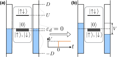
Model. We consider a quantum dot attached to two metallic leads, schematically shown in Fig. 1. Both the quantum dot and the leads are initially in thermal equilibrium at temperature . We describe the system by an Anderson impurity model
| (1a) | ||||
| (1b) | ||||
| (1c) | ||||
and label electrons in the leads and on the dot, respectively, is the spin index, labels the left and right lead. is the tunneling matrix element between impurity and leads, is the lead dispersion, the impurity level spacing, and the impurity electronic repulsion strength (charging energy). The chemical potential is set to at equilibrium, the instantaneous (quenched) application of voltage at time changes it to .
The leads are non-interacting and are described by a flat density of states with half-bandwidth and a smooth cutoff at the band edges Werner et al. (2010). The coupling of the dot and leads is described by the effective coupling parameter and the hybridization function
| (2) |
denotes the integral over the L-shaped Keldysh contour with an imaginary branch added to take into account the initial correlated conditions Rammer and Smith (1986), and is the Fermi function.
We describe the evolution of the system by a hybridization expansion in the tunneling term , which we stochastically sum to all orders using diagrammatic continuous-time Monte Carlo (CT-HYB) on the full Keldysh contour Werner et al. (2006, 2009); Schiró (2010). We perform an expansion for the partition function of the problem , where every perturbation order of expansion in is characterized by configurations consisting of operators distributed on the contour and the impurity state . Summing the series stochastically allows one to extract the time-dependence of the quantum dot charge Gull et al. (2011b) as , where , is the Monte Carlo sign of every configuration and is the average sign. The sign is equal to in equilibrium, but decays exponentially with real time. In practice we resolve times of order of . Calculations at larger times are exponentially more expensive.
The main observable of interest is the current passing through the dot. The QMC procedure should be modified for current calculations by replacing with and sampling the imaginary part of the weight of every configuration, yielding Werner et al. (2009). From this we extract the quantity and, by dividing by , the current.
In order to evaluate the current separate measurements of and are required. These quantities are not directly accessible by QMC, but are instead inferred from a normalization procedure, yielding
| (3) |
where and are the partition function and the current of a reference system, which are obtained separately. Each of the fractions in Eq. (3) is obtained in a CT-HYB calculation as
| (4) |
The choice of the reference system is important: small ratios of and results in large relative error bars. As temperature is decreased, the average perturbation order increases , and the normalization to the first order of expansion in Werner et al. (2009) becomes unreliable. We improve the algorithm in several ways: first, at high temperatures (perturbation orders ) the reference system is a finite order NCA/OCA expansion. At lower temperatures (larger pertubation orders) we perform a series of calculations, progressively increasing the perturbation order until convergence is achieved, yielding
| (5) |
with the order of the NCA expansion and as either or to maintain ratios at every step. We emphasize that our results are exact within the stochastic error bars for any choice of reference system; the choice affects only the computational cost.
Results. We present results for the dynamics of a quantum dot in the mixed valence regime, . The Kondo temperature is on the order of the coupling Goldhaber-Gordon et al. (1998), and observables are expected to equilibrate within times , accessible by QMC calculations Werner et al. (2009); Gull et al. (2010, 2011b). For convenient comparison to experiment we set the unit of energy close to meV. Time is then given in meV ps. We parametrize the setup with a coupling of , a charging energy () and a half-bandwidth () similar to Ref. Keller et al., 2013. Band cutoff effects at are expected not to play a role in the dynamics Werner et al. (2010); Hewson (1993).
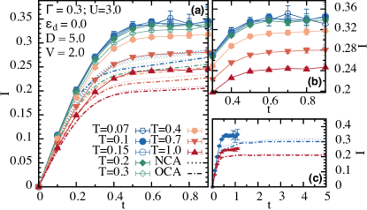
Fig. 2 shows the behavior of the current after a voltage quench. In panel (a) we show as a function of time following a voltage quench from to for a set of temperatures (between and K). Results from semi-analytical approximations are shown as fine dotted lines (NCA) and dash-dotted lines (OCA) for comparison Aoki et al. (2014); Eckstein and Werner (2010). We observe that for all temperatures the current equilibrates at time ( ps) well within reachable times of ( ps). As temperature is lowered from ( K) to ( K) the current at fixed times and in steady state increases. Further reducing by a factor of five yields no additional increase of current, illustrated by panel (b). We attribute the fast equilibration time to the high Kondo temperature of this mixed valence system Gull et al. (2011b).
Results from NCA and OCA correctly capture the short-time behavior and the overall shape of the current but underestimate both the transient and the steady state value by . This is known for systems with Haule et al. (2001), although the quality of these methods will presumably improve in the strong interaction limit and by including vertex corrections in OCA Tosi et al. (2011). Both results are shown in panel (c) for times much longer than presently accessible by QMC. No additional time-dependence is visible, illustrating that our calculations are able to reach steady state.
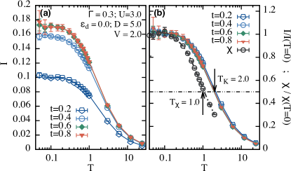
The temperature dependence of the current is analyzed in Fig. 3. The saturation of the low- current is clearly visible in panel (a), where different traces show the transient current obtained at different times. We identify the saturation of the current in the low- regime with Kondo behavior and the temperature at which the current reaches half of its saturated low- value as the Kondo temperature Hewson (1993); Costi et al. (1994).
Fig. 3b shows the temperature dependence of the current and equilibrium magnetic susceptibility normalized to the respective zero-temperature values. The magnetic susceptibility, defined as a response to the infinitesimal local magnetic field , saturates at low temperatures Hewson (1993); Hanl and Weichselbaum (2014), similarly to the current. For all normalized current values for different times collapse on a single curve. This shows that Kondo behavior can be detected based purely on short-time transient dynamics. The Kondo temperature determined by the current is time-independent and occurs at around twice the value of as defined from the point where the equilibrium magnetic susceptibility reaches half of its zero- value, as expected in a mixed-valence regime Goldhaber-Gordon et al. (1998); Yoshida et al. (2009); Smirnov and Grifoni (2013).
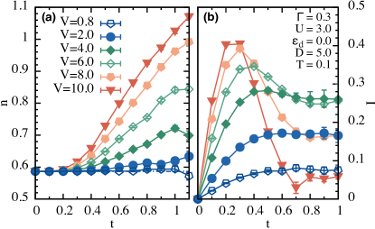
We proceed with studying the impact of the magnitude of the applied bias voltage. Fig. 4 shows the time dependence of the quantum dot occupancy (a) and current (b) at a range of voltages between and . At voltages (linear response) the occupancy retains its equilibrium value and the current shows a monotonic rise and saturation to the steady state value, which increases with the applied voltage. Larger voltages demonstrate linear response behavior only at small times . At larger times the nonlinear behavior is visible: the current decreases to the steady state value, which becomes smaller with applied , illustrating the breakdown of conductance at large voltages 111At the current decays to zero and oscillates with the period (not shown). .
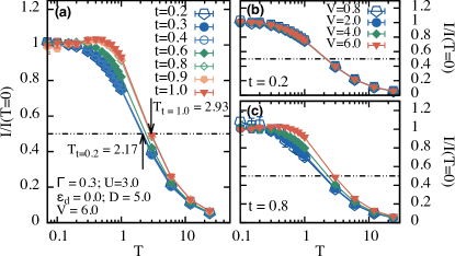
The temperature dependence of the current outside of the linear response regime is analyzed in Fig. 5. Panel (a) shows at as a function of temperature . Different traces show different transient times, between ( ps) and ( ps). Similarly to the linear response case (Fig. 3), the current exhibits the low temperature saturation at all times. The Kondo effect is therefore visible in transient dynamics for all voltages. Outside linear response, the temperature at which the current saturates is strongly time-dependent. We denote the characteristic saturation temperature as and define as before . At short times (panel (b)) is the Kondo temperature for all voltages. As time increases increases by and reaches its steady state value of for (c). Further increase of the voltage results in a non-monotonic temperature dependence of the current Reininghaus et al. (2014) (not shown).
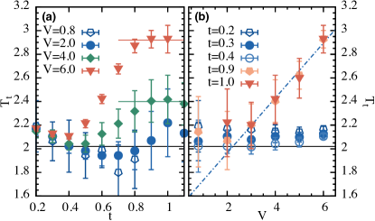
In Fig. 6 we show the time (a) and voltage (b) evolution of . For small voltages, there is no time-dependence of . In contrast, as is increased up to , rapidly rises and equilibrates. Estimates of the steady-state as defined by the value at which the current reaches half of its low- value for are given by the horizontal lines. Fig. 6b shows a separation of short- and long-time behavior: no change in is observed for short times ( ps), whereas in the steady state is found to be increasing with for in agreement with experiments Kretinin et al. (2011) and predictions from the real time renormalization group Reininghaus et al. (2014).
Conclusions. We have described the transient dynamics of a quantum dot in the mixed valence regime following the instantaneous application of a bias voltage in a range of temperatures below and above the Kondo temperature . We have observed the full dynamics of the system from equilibrium to steady state. At all times and all voltages below the lead bandwidth, the current saturates at low temperature, exhibiting Kondo behavior. In linear response the saturation temperature at which the current reaches half of its zero-temperature value is the Kondo temperature . Outside of the linear response regime has a strong time dependence and connects the equilibrium Kondo temperature to the increased steady state value Reininghaus et al. (2014); Kretinin et al. (2011). The temperature describes the interplay of non-equilibrium (applied voltage) and strong correlations in the system.
The results presented here are exact within the error-bars and the current and time-dependent are directly accessible in time-resolved experiments Nunes and Freeman (1993); Loth et al. (2010). The dynamics of the mixed valence system is fast - the equilibration occurs on a picosecond scale. We believe that the same physics can be observed at much larger time scales by lowering the level spacing and, consequently, entering the Kondo regime, thereby decreasing and exponentially increasing the relaxation time Gull et al. (2011b).
Acknowledgements.
The authors acknowledge helpful discussions with Lucas Peeters, Guy Cohen, James P. F. LeBlanc, H. Terletska, and Pedro Ribeiro, and thank DOE ER 46932 for financial support. We have used ALPSCore Bauer et al. (2011); Gaenko et al. (2015) and GFTools libraries Antipov (2015) for the programming development. This research used resources of the National Energy Research Scientific Computing Center, a DOE Office of Science User Facility supported by the Office of Science of the U.S. Department of Energy under Contract No. DE-AC02-05CH11231.References
- Kondo (1964) J. Kondo, Prog. Theor. Phys. 32, 37 (1964).
- Abrikosov (1965) A. A. Abrikosov, Sov. Phys. JETP 21, 660 (1965).
- Suhl (1965) H. Suhl, Phys. Rev. 138, A515 (1965).
- Costi et al. (1994) T. A. Costi, A. C. Hewson, and V. Zlatic, J. Phys. Condens. Matter 6, 2519 (1994).
- Konik et al. (2001) R. M. Konik, H. Saleur, and A. W. W. Ludwig, Phys. Rev. Lett. 87, 236801 (2001).
- Madhavan (1998) V. Madhavan, Science 280, 567 (1998).
- Knorr et al. (2002) N. Knorr, M. A. Schneider, L. Diekhöner, P. Wahl, and K. Kern, Phys. Rev. Lett. 88, 096804 (2002).
- Park et al. (2002) J. Park, A. N. Pasupathy, J. I. Goldsmith, C. Chang, Y. Yaish, J. R. Petta, M. Rinkoski, J. P. Sethna, H. D. Abruña, P. L. McEuen, and D. C. Ralph, Nature 417, 722 (2002).
- Gegenwart et al. (2008) P. Gegenwart, Q. Si, and F. Steglich, Nat. Phys. 4, 186 (2008).
- Schopfer et al. (2003) F. Schopfer, C. Bäuerle, W. Rabaud, and L. Saminadayar, Phys. Rev. Lett. 90, 056801 (2003).
- Goldhaber-Gordon et al. (1998) D. Goldhaber-Gordon, J. Göres, M. A. Kastner, H. Shtrikman, D. Mahalu, and U. Meirav, Phys. Rev. Lett. 81, 5225 (1998).
- Kouwenhoven and Glazman (2001) L. Kouwenhoven and L. Glazman, Phys. World 14, 33 (2001).
- Jeong et al. (2001) H. Jeong, A. M. Chang, and M. R. Melloch, Science 293, 2221 (2001).
- De Franceschi et al. (2002) S. De Franceschi, R. Hanson, W. G. van der Wiel, J. M. Elzerman, J. J. Wijpkema, T. Fujisawa, S. Tarucha, and L. P. Kouwenhoven, Phys. Rev. Lett. 89, 156801 (2002).
- Wilson (1975) K. G. Wilson, Rev. Mod. Phys. 47, 773 (1975).
- Hewson (1993) A. C. Hewson, The Kondo Problem to Heavy Fermions (Cambridge University Press, New York, N.Y., 1993).
- Bulla et al. (2008) R. Bulla, T. A. Costi, and T. Pruschke, Rev. Mod. Phys. 80, 395 (2008).
- Schollwöck (2005) U. Schollwöck, Rev. Mod. Phys. 77, 259 (2005).
- Hirsch and Fye (1986) J. E. Hirsch and R. M. Fye, Phys. Rev. Lett. 56, 2521 (1986).
- Gull et al. (2011a) E. Gull, A. J. Millis, A. I. Lichtenstein, A. N. Rubtsov, M. Troyer, and P. Werner, Rev. Mod. Phys. 83, 349 (2011a).
- Rubtsov et al. (2005) A. N. Rubtsov, V. V. Savkin, and A. I. Lichtenstein, Phys. Rev. B 72, 035122 (2005).
- Werner et al. (2006) P. Werner, A. Comanac, L. de’ Medici, M. Troyer, and A. J. Millis, Phys. Rev. Lett. 97, 076405 (2006).
- Meir et al. (1993) Y. Meir, N. S. Wingreen, and P. A. Lee, Phys. Rev. Lett. 70, 2601 (1993).
- Fujii and Ueda (2003) T. Fujii and K. Ueda, Phys. Rev. B 68, 155310 (2003).
- Plihal et al. (2005) M. Plihal, D. C. Langreth, and P. Nordlander, Phys. Rev. B 71, 165321 (2005).
- Han and Heary (2007) J. E. Han and R. J. Heary, Phys. Rev. Lett. 99, 236808 (2007).
- Fritsch and Kehrein (2010) P. Fritsch and S. Kehrein, Phys. Rev. B 81, 035113 (2010).
- Dirks et al. (2010) A. Dirks, P. Werner, M. Jarrell, and T. Pruschke, Phys. Rev. E 82, 026701 (2010).
- Mitra and Rosch (2011) A. Mitra and A. Rosch, Phys. Rev. Lett. 106, 106402 (2011).
- Dorda et al. (2014) A. Dorda, M. Nuss, W. von der Linden, and E. Arrigoni, Phys. Rev. B 89, 165105 (2014).
- Cohen et al. (2014a) G. Cohen, E. Gull, D. R. Reichman, and A. J. Millis, Phys. Rev. Lett. 112, 146802 (2014a).
- Dirks et al. (2013) A. Dirks, S. Schmitt, J. E. Han, F. Anders, P. Werner, and T. Pruschke, Europhys. Lett. 102, 37011 (2013).
- Rosch et al. (2005) A. Rosch, J. Paaske, J. Kroha, and P. Wölfle, J. Phys. Soc. Japan 74, 118 (2005).
- Kaminski et al. (2000) A. Kaminski, Y. V. Nazarov, and L. I. Glazman, Phys. Rev. B 62, 18 (2000).
- Kretinin et al. (2012) A. V. Kretinin, H. Shtrikman, and D. Mahalu, Phys. Rev. B 85, 201301 (2012).
- Smirnov and Grifoni (2013) S. Smirnov and M. Grifoni, Phys. Rev. B 87, 121302 (2013).
- Wingreen and Meir (1994) N. S. Wingreen and Y. Meir, Phys. Rev. B 49, 11040 (1994).
- Kretinin et al. (2011) A. V. Kretinin, H. Shtrikman, D. Goldhaber-Gordon, M. Hanl, A. Weichselbaum, J. von Delft, T. Costi, and D. Mahalu, Phys. Rev. B 84, 245316 (2011).
- Reininghaus et al. (2014) F. Reininghaus, M. Pletyukhov, and H. Schoeller, Phys. Rev. B 90, 085121 (2014).
- Latta et al. (2011) C. Latta, F. Haupt, M. Hanl, A. Weichselbaum, M. Claassen, W. Wuester, P. Fallahi, S. Faelt, L. Glazman, J. von Delft, H. E. Türeci, and A. Imamoglu, Nature 474, 627 (2011).
- Türeci et al. (2011) H. E. Türeci, M. Hanl, M. Claassen, A. Weichselbaum, T. Hecht, B. Braunecker, A. Govorov, L. Glazman, A. Imamoglu, and J. von Delft, Phys. Rev. Lett. 106, 107402 (2011).
- Nunes and Freeman (1993) G. Nunes and M. R. Freeman, Science 262, 1029 (1993).
- Loth et al. (2010) S. Loth, M. Etzkorn, C. P. Lutz, D. M. Eigler, and A. J. Heinrich, Science 329, 1628 (2010).
- Terada et al. (2010) Y. Terada, S. Yoshida, O. Takeuchi, and H. Shigekawa, Nat. Photonics 4, 869 (2010).
- Yoshida et al. (2014) S. Yoshida, Y. Aizawa, Z.-H. Wang, R. Oshima, Y. Mera, E. Matsuyama, H. Oigawa, O. Takeuchi, and H. Shigekawa, Nat. Nanotechnol. 9, 588 (2014).
- Weiss et al. (2008) S. Weiss, J. Eckel, M. Thorwart, and R. Egger, Phys. Rev. B 77, 195316 (2008).
- Segal et al. (2010) D. Segal, A. J. Millis, and D. R. Reichman, Phys. Rev. B 82, 205323 (2010).
- Eckel et al. (2010) J. Eckel, F. Heidrich-Meisner, S. G. Jakobs, M. Thorwart, M. Pletyukhov, and R. Egger, New J. Phys. 12, 043042 (2010).
- Becker et al. (2012) D. Becker, S. Weiss, M. Thorwart, and D. Pfannkuche, New J. Phys. 14, 073049 (2012).
- Hützen et al. (2012) R. Hützen, S. Weiss, M. Thorwart, and R. Egger, Phys. Rev. B 85, 121408 (2012).
- Weiss et al. (2013) S. Weiss, R. Hützen, D. Becker, J. Eckel, R. Egger, and M. Thorwart, Phys. Status Solidi B 250, 2298 (2013).
- Schoeller (2009) H. Schoeller, Eur. Phys. J. Spec. Top. 168, 179 (2009).
- Andergassen et al. (2011) S. Andergassen, M. Pletyukhov, D. Schuricht, H. Schoeller, and L. Borda, Phys. Rev. B 83, 205103 (2011).
- Kennes and Meden (2012) D. M. Kennes and V. Meden, Phys. Rev. B 85, 245101 (2012), arXiv:arXiv:1204.2100v1 .
- Zheng et al. (2009) X. Zheng, J. Jin, S. Welack, M. Luo, and Y. Yan, J. Chem. Phys. 130, 164708 (2009).
- Härtle and Millis (2014) R. Härtle and A. J. Millis, Phys. Rev. B 90, 245426 (2014).
- Härtle et al. (2015) R. Härtle, G. Cohen, D. R. Reichman, and A. J. Millis, (2015), arXiv:1505.01283 .
- Wang and Kehrein (2010) P. Wang and S. Kehrein, Phys. Rev. B 82, 125124 (2010).
- Heyl and Kehrein (2010) M. Heyl and S. Kehrein, J. Phys. Condens. Matter 22, 345604 (2010).
- Ratiani and Mitra (2010) Z. Ratiani and A. Mitra, Phys. Rev. B 81, 125110 (2010).
- Hara et al. (2015) B. Hara, A. Koga, and T. Aono, Phys. Rev. B 92, 081103 (2015).
- Schiró and Fabrizio (2010) M. Schiró and M. Fabrizio, Phys. Rev. Lett. 105, 076401 (2010).
- Lanatà and Strand (2012) N. Lanatà and H. U. R. Strand, Phys. Rev. B 86, 115310 (2012).
- White and Feiguin (2004) S. R. White and A. E. Feiguin, Phys. Rev. Lett. 93, 076401 (2004).
- Daley et al. (2004) A. J. Daley, C. Kollath, U. Schollwoeck, and G. Vidal, J. Stat. Mech. Theory Exp. 2004, 27 (2004).
- Anders and Schiller (2006) F. B. Anders and A. Schiller, Phys. Rev. B 74, 245113 (2006).
- Schmidt et al. (2008) T. L. Schmidt, P. Werner, L. Mühlbacher, and A. Komnik, Phys. Rev. B 78, 235110 (2008).
- Werner et al. (2009) P. Werner, T. Oka, and A. J. Millis, Phys. Rev. B 79, 035320 (2009).
- Mühlbacher et al. (2011) L. Mühlbacher, D. F. Urban, and A. Komnik, Phys. Rev. B 83, 075107 (2011).
- Koga (2013) A. Koga, Phys. Rev. B 87, 115409 (2013).
- Gull et al. (2010) E. Gull, D. R. Reichman, and A. J. Millis, Phys. Rev. B 82, 075109 (2010).
- Gull et al. (2011b) E. Gull, D. R. Reichman, and A. J. Millis, Phys. Rev. B 84, 085134 (2011b).
- Cohen et al. (2014b) G. Cohen, D. R. Reichman, A. J. Millis, and E. Gull, Phys. Rev. B 89, 115139 (2014b).
- Cohen et al. (2013) G. Cohen, E. Gull, D. R. Reichman, A. J. Millis, and E. Rabani, Phys. Rev. B 87, 195108 (2013).
- Lechtenberg and Anders (2014) B. Lechtenberg and F. B. Anders, Phys. Rev. B 90, 045117 (2014).
- Nuss et al. (2015) M. Nuss, M. Ganahl, E. Arrigoni, W. von der Linden, and H. G. Evertz, Phys. Rev. B 91, 085127 (2015).
- Werner et al. (2010) P. Werner, T. Oka, M. Eckstein, and A. J. Millis, Phys. Rev. B 81, 035108 (2010).
- Schiró (2010) M. Schiró, Phys. Rev. B 81, 085126 (2010).
- Härtle et al. (2013) R. Härtle, G. Cohen, D. R. Reichman, and A. J. Millis, Phys. Rev. B 88, 235426 (2013).
- Ye et al. (2015) L. Ye, D. Hou, X. Zheng, Y. Yan, and M. Di Ventra, Phys. Rev. B 91, 205106 (2015).
- Cheng et al. (2015) Y. Cheng, W. Hou, Y. Wang, Z. Li, J. Wei, and Y. Yan, New J. Phys. 17, 033009 (2015).
- Kirino et al. (2008) S. Kirino, T. Fujii, J. Zhao, and K. Ueda, J. Phys. Soc. Japan 77, 084704 (2008).
- Heidrich-Meisner et al. (2009) F. Heidrich-Meisner, A. E. Feiguin, and E. Dagotto, Phys. Rev. B 79, 235336 (2009).
- Kirino and Ueda (2011) S. Kirino and K. Ueda, Ann. Phys. 523, 664 (2011).
- Anders (2008) F. B. Anders, Phys. Rev. Lett. 101, 066804 (2008).
- Eidelstein et al. (2012) E. Eidelstein, A. Schiller, F. Güttge, and F. B. Anders, Phys. Rev. B 85, 075118 (2012).
- Nghiem and Costi (2014) H. T. M. Nghiem and T. A. Costi, Phys. Rev. B 89, 075118 (2014).
- Goker et al. (2010) A. Goker, Z. Y. Zhu, A. Manchon, and U. Schwingenschlögl, Phys. Rev. B 82, 161304 (2010).
- Oguri and Sakano (2013) A. Oguri and R. Sakano, Phys. Rev. B 88, 155424 (2013).
- Eckstein and Werner (2010) M. Eckstein and P. Werner, Phys. Rev. B 82, 115115 (2010).
- Aoki et al. (2014) H. Aoki, N. Tsuji, M. Eckstein, M. Kollar, T. Oka, and P. Werner, Rev. Mod. Phys. 86, 779 (2014).
- Haule et al. (2001) K. Haule, S. Kirchner, J. Kroha, and P. Wölfle, Phys. Rev. B 64, 155111 (2001).
- Tosi et al. (2011) L. Tosi, P. Roura-Bas, A. M. Llois, and L. O. Manuel, Phys. Rev. B 83, 073301 (2011).
- Rammer and Smith (1986) J. Rammer and H. Smith, Rev. Mod. Phys. 58, 323 (1986).
- Keller et al. (2013) A. J. Keller, S. Amasha, I. Weymann, C. P. Moca, I. G. Rau, J. A. Katine, H. Shtrikman, G. Zaránd, and D. Goldhaber-Gordon, Nat. Phys. 10, 145 (2013).
- Hanl and Weichselbaum (2014) M. Hanl and A. Weichselbaum, Phys. Rev. B 89, 075130 (2014).
- Yoshida et al. (2009) M. Yoshida, A. C. Seridonio, and L. N. Oliveira, Phys. Rev. B 80, 235317 (2009).
- Note (1) At the current decays to zero and oscillates with the period (not shown).
- Bauer et al. (2011) B. Bauer, L. D. Carr, H. G. Evertz, A. Feiguin, J. Freire, S. Fuchs, L. Gamper, J. Gukelberger, E. Gull, S. Guertler, A. Hehn, R. Igarashi, S. V. Isakov, D. Koop, P. N. Ma, P. Mates, H. Matsuo, O. Parcollet, G. Pawłowski, J. D. Picon, L. Pollet, E. Santos, V. W. Scarola, U. Schollwöck, C. Silva, B. Surer, S. Todo, S. Trebst, M. Troyer, M. L. Wall, P. Werner, and S. Wessel, J. Stat. Mech. Theory Exp. 2011, P05001 (2011).
- Gaenko et al. (2015) A. Gaenko, A. E. Antipov, and E. Gull, “ALPSCore : Libraries for Physics Simulations,” (2015).
- Antipov (2015) A. E. Antipov, “GFTools : a domain-specific language for Green’s function calculations,” (2015).