Order and excitations in large-$S$ kagomé-lattice antiferromagnets

Abstract

We systematically investigate the ground-state and the spectral properties of antiferromagnets on a kagomé lattice with several common types of the planar anisotropy: $XXZ$, single-ion, and out-of-plane Dzyaloshinskii-Moriya. Our main focus is on the role of nonlinear, anharmonic terms, which are responsible for the quantum order-by-disorder effect and for the corresponding selection of the ground-state spin structure in many of these models. The $XXZ$ and the single-ion anisotropy models exhibit a quantum phase transition between the ${\bf q}\!=\!0$ and the $\sqrt{3}\times\!\sqrt{3}$ states as a function of the anisotropy parameter, offering a rare example of the quantum order-by-disorder fluctuations favoring a ground state which is different from the one selected by thermal fluctuations. The nonlinear terms are also shown to be crucial for a very strong near-resonant decay phenomenon leading to the quasiparticle breakdown in the kagomé-lattice antiferromagnets whose spectra are featuring flat or weakly dispersive modes. The effect is shown to persist even in the limit of large spin values and should be common to other frustrated magnets with flat branches of excitations. Model calculations of the spectrum of the $S=5/2$ Fe-jarosite with Dzyaloshinskii-Moriya anisotropy provide a convincing and detailed characterization of the proposed scenario.

I Introduction

Kagomé-lattice antifferomagnets are iconic in the field of frustrated magnets, comprising a number of model systems whose classical ground states are massively degenerate, giving rise to an extreme sensitivity to subtle symmetry breaking effects,Huse92 ; Chalker92 to fractional magnetization plateaus, MZH02 ; Capponi13 to a strongly amplified role of secondary interactions,Harris92 and to an emergent hierarchy of energy scales in their dynamics.Taillefumier14 A crucial role of the non-linear, anharmonic terms in the so-called order-by-disorder ground-state selection by thermalReimers93 or quantum fluctuationsChubukov92 in the kagomé-lattice antifferomagnets has been recognized for some time. Recently, an accurate, systematic treatment of the quantum order-by-disorder effect in the anisotropic versions of the model has received a significant development.ChZh14 ; Gotze15 However, much less is known about the role of such terms in the excitation spectra of frustrated magnets and only recently a rather dramatic picture has begun to emerge. Ch15

Usually, the nonlinear terms in antiferromagnets are necessary to describe interactions of magnons and, while their role is, generally, more significant when frustration is present,RMP13 ; triPRB09 they still lead to effects that are relatively minor in the large-$S$ limit, i.e., constitute a $1/S$ contribution compared with the classical energy scale $JS$. However, in a wide class of highly-frustrated systems, including the kagomé-lattice antiferromagnets, the non-linear anharmonic terms are responsible for the phenomena that are much more dramatic.

First effect concerns systems in which contenders for the ground state form a highly degenerate, extensive manifold of states, and neither the classical energetics nor the harmonic fluctuations are able to select a unique ground state from that manifold.Chalker92 ; Chubukov92 ; Harris92 In that case, the selection role is passed onto the nonlinear terms providing a variant of the quantum order by disorder effect. Such is the case of the three models considered in this work, Heisenberg, $XXZ$,ChZh14 and single-ion anisotropy models, while in the case of the Dzyaloshinskii-Moriya (DM) anisotropy, a unique state is selected already on the classical level.Cepas08

The second effect is less-studied, but is equally striking. We demonstrate, that the nonlinear terms lead to spectacularly strong quantum effects in the dynamical response of the flat-band frustrated magnets, even in the ones that are assumed nearly classical.Ch15 The resultant spectral features invoke parallels with the quasiparticle breakdown signatures in quantum spin- and Bose-liquids,Zaliznyak ; Zheludev which exhibit termination points and broad continua where single-particle excitations are no longer well-defined. In the present case, the origin of such features is in the near-resonant decay into pairs of the flat modes, facilitated by the nonlinear couplings. The effect is strongly amplified by the density of states of the flat modes and can be shown to persist even in the large-$S$ limit, defying the usual $1/S$ suppression trend and challenging a conventional wisdom that such drastic phenomena can only occur in an inherently quantum system.

In the present study, we expand the analysis of our previous worksChZh14 ; Ch15 and offer an exposé of the $1/S$ formalism for several common anisotropic extensions of the nearest-neighbor Heisenberg model on the kagomé lattice that are also relevant to real materials. The presented approach to the nonlinear spin-wave theory can be applicable to the other, more complicated forms of the kagomé-lattice Hamiltonians as well as to a broader class of frustrated spin systems on the non-Bravais lattices. We also provide a useful extension of our approach to the perturbative treatment of small perturbations to the main Hamiltonian, such as the next-nearest superexchanges $J_{2}$.

For the ground-state consideration, we demonstrate a quantum phase transition between the ${\bf q}\!=\!0$ and the $\sqrt{3}\times\!\sqrt{3}$ states as a function of anisotropy parameter in two models: $XXZ$ model, studied previously,ChZh14 and the single-ion anisotropy model. While the effect is similar in both models, the energy scale associated with it is shown to be different, in agreement with the understanding that the degeneracy-lifting interaction is associated with a high-order topologically-nontrivial spin-flip processes, which are different in the two models. Nevertheless, both model cases present a rare example of the ground-state selection that is different from the choice of the thermal fluctuations, which favor the $\sqrt{3}\times\!\sqrt{3}$ structure for any value of the anisotropy parameter. Harris92 ; Reimers93 ; Henley09 ; Huse92 ; Korshunov02 ; Rzchowski97 ; ChZh14 ; Gotze15

For the spectral properties of the kagomé-lattice antiferromagnets, we offer a detailed consideration of the decay-induced effects in the DM anisotropy model with $J_{2}$, the model that closely describes the $S=5/2$ Fe-jarosite.Matan06 ; Yildirim06 We also present a general analysis of the near-resonant decays in the flat-band frustrated antiferromagnets, which suggests that the dramatic modifications in the spectrum due to this phenomenon must persist in the large-$S$ limit. While the core of our presentation is aimed at a common and realistic extension of the nearest-neighbor Heisenberg kagomé-lattice antiferromagnet, we argue that the spectacularly strong quantum effect of the quasiparticle breakdown in an almost classical system should be applicable to a variety of other flat-band frustrated spin systems. Petrenko ; Matan14 ; Balents_honeycomb ; Georgii15 We also remark on a useful ${\bf q}$-dependence of the dynamical structure factor, which is characteristic to the non-Bravais lattices and allows to select spectral contributions of specific branches in the portions of the ${\bf q}$-space.

The paper is organized as follows. In Sec. II we present a consideration of the harmonic theory for several common anisotropic models on the kagomé lattice, explicate details of the diagonalization procedure, and show results of a representative calculation within the harmonic approximation. In Sec. III, anharmonic terms of the models are derived and the results of the ground-state selection calculations are presented. The spectral properties of the kagomé-lattice antiferromagnets are also given a detailed exposition. Technical aspects of the derivation of the quartic terms are given in Appendix A.

II Linear spin-wave theory

To set the stage, we provide the linear spin-wave consideration of the isotropic nearest-neighbor antiferromagnetic Heisenberg model on the kagomé lattice following the approach of Ref. Harris92, . We continue with various extensions of the model, which are either relevant to real materials or allow to explore the role of quantum effects in a wider parameter space. These extensions include the anisotropic $XXZ$ model, models with the single-ion and the out-of-plane Dzyaloshinskii-Moria anisotropies, and additional further-neighbor exchange terms. Subsequently, the important steps of the diagonalization procedure that will be essential for the non-linear terms considered in Sec. III are exposed. In the end of this Section, results of the calculations of the on-site magnetization within the linear spin-wave theory for the $XXZ$ model are presented as an example.

II.1 Nearest-neighbor Heisenberg model

Within the spin-wave treatment, nearest-neighbor Heisenberg antiferromagnet on the kagomé lattice with the Hamiltonian

$$\hat{\cal H}=J\sum_{\langle ij\rangle}{\bf S}_{i}\cdot{\bf S}_{j}\ ,$$ (1)

is assumed to be in an ordered state with spins forming a coplanar 120^∘ structure. Summation is over bonds and $i,j$ are the sites of the lattice. Aligning the $z$-axis on each site along the direction of the ordered moment and directing the $y$-axes out of the ordering plane transforms the Hamiltonian (1) to a local spin basis

$$\hat{\cal H} = J\sum_{\langle ij\rangle}\Bigl{(}S_{i}^{y}S_{j}^{y}+\cos\theta_{ij}\left(S_{i}^{x}S_{j}^{x}+S_{i}^{z}S_{j}^{z}\right)$$ (2)

$$+\sin\theta_{ij}\left(S_{i}^{z}S_{j}^{x}-S_{i}^{x}S_{j}^{z}\right)\Bigr{)}=J\sum_{\langle ij\rangle}{\bf S}_{i}\otimes{\bf S}_{j}\ ,$$

where $\theta_{ij}=\theta_{i}-\theta_{j}$ is an angle between two neighboring spins and we have introduced “matrix” product $\otimes$ of spins with the matrix

$$\otimes=\left(\begin{array}[]{ccc}\cos\theta_{ij}&0&-\sin\theta_{ij}\\ 0&1&0\\ \sin\theta_{ij}&0&\cos\theta_{ij}\end{array}\right)\,$$ (3)

as a shorthand notation.

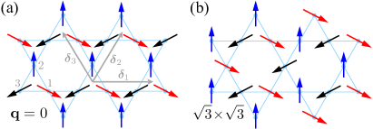
Figure 1: (Color online) (a) ${\bf q}\!=\!0$ and (b) $\sqrt{3}\times\!\sqrt{3}$ spin configurations. In (a), primitive vectors of the kagomé lattice and numbering of sites within the unit cell are shown.

We choose the unit cell of the kagomé lattice as an up-triangle, see Fig. 1, and the primitive vectors of the corresponding triangular Bravais lattice as

$$\bm{\delta}_{1}=(1,0)\,,\ \bm{\delta}_{2}=\biggl{(}\frac{1}{2},\frac{\sqrt{3}}{2}\biggr{)}\,,\ \bm{\delta}_{3}=\bm{\delta}_{2}-\bm{\delta}_{1}\,,$$ (4)

all in units of $2a$ where $a$ is the interatomic distance. The atomic coordinates within the unit cell are $\bm{\rho}_{1}=0$, $\bm{\rho}_{2}=\frac{1}{2}\bm{\delta}_{3}$, and $\bm{\rho}_{3}=-\frac{1}{2}\bm{\delta}_{1}$.

Then, changing summation over bonds to summation over unit cells and the atomic index, $i\rightarrow\{\alpha,\ell\}$, with $\alpha=1$–3 enumerating atoms within the unit cell, the Hamiltonian (2) becomes

$$\hat{\cal H} = J\sum_{\ell}{\bf S}_{1,\ell}\otimes\left({\bf S}_{2,\ell}+{\bf S}_{2,\ell-3}\right)$$

$$+{\bf S}_{1,\ell}\otimes\left({\bf S}_{3,\ell}+{\bf S}_{3,\ell+1}\right)+{\bf S}_{2,\ell}\otimes\left({\bf S}_{3,\ell}+{\bf S}_{3,\ell+2}\right)\,,$$

where the product ${\bf S}_{\alpha,\ell}\otimes{\bf S}_{\alpha^{\prime},\ell^{\prime}}$ is according to (2), and $\ell\pm n\equiv{\bf R}_{\ell}\pm\bm{\delta}_{n}$ with the coordinate of the unit cell ${\bf R}_{\ell}=m_{1}\bm{\delta}_{1}+m_{2}\bm{\delta}_{2}$.

II.2 Harmonic spin-wave approximation

It should be noted that although a coplanar state with spins on each triangle in a 120^∘ structure minimizes the classical energy of (1), such a state is not unique and the manifold of them is extensive.Baxter70 However, it is also clear from the Hamiltonian in the local basis (2) that the linear spin-wave theory is the same for any state from this degenerate manifold,Chalker92 because $\cos\theta_{ij}=-1/2$ for any pair of spins in such state and $S^{x}S^{z}$ terms do not contribute to the harmonic order of the $1/S$ expansion.

Thus, we introduce Holstein-Primakoff representation for spin operators

$$S_{\alpha,\ell}^{z}=S-a^{\dagger}_{\alpha,\ell}a^{\phantom{{\dagger}}}_{\alpha,\ell}\ ,\ \ S_{\alpha,\ell}^{-}=a_{\alpha,\ell}^{\dagger}\sqrt{2S-a^{\dagger}_{\alpha,\ell}a^{\phantom{{\dagger}}}_{\alpha,\ell}}$$ (6)

into (II.1) and, keeping only quadratic terms, obtain a harmonic Hamiltonian for three species of bosons

$$\hat{\cal H}_{2} = 2JS\sum_{\ell}\biggl{\{}\Bigl{[}a_{1,\ell}^{\dagger}a^{\phantom{{\dagger}}}_{1,\ell}+a_{2,\ell}^{\dagger}a^{\phantom{{\dagger}}}_{2,\ell}+a_{3,\ell}^{\dagger}a^{\phantom{{\dagger}}}_{3,\ell}\Bigr{]}$$

$$+ \frac{1}{8}\Bigl{[}a_{1,\ell}^{\dagger}\bigl{(}a^{\phantom{{\dagger}}}_{2,\ell}+a^{\phantom{{\dagger}}}_{2,\ell-3}\bigr{)}+a_{1,\ell}^{\dagger}\bigl{(}a^{\phantom{{\dagger}}}_{3,\ell}+a^{\phantom{{\dagger}}}_{3,\ell+1}\bigr{)}$$

$$\phantom{\frac{1}{8}\Bigl{[}}+\,a_{2,\ell}^{\dagger}\bigl{(}a^{\phantom{{\dagger}}}_{3,\ell}+a^{\phantom{{\dagger}}}_{3,\ell+2}\bigr{)}+\textrm{h.c.}\Bigr{]}$$

$$- \frac{3}{8}\Bigl{[}a^{\phantom{{\dagger}}}_{1,\ell}\bigl{(}a^{\phantom{{\dagger}}}_{2,\ell}+a^{\phantom{{\dagger}}}_{2,\ell-3}\bigr{)}+a^{\phantom{{\dagger}}}_{1,\ell}\bigl{(}a^{\phantom{{\dagger}}}_{3,\ell}+a^{\phantom{{\dagger}}}_{3,\ell+1}\bigr{)}$$

$$\phantom{\frac{3}{8}\Bigl{[}}+\,a^{\phantom{{\dagger}}}_{2,\ell}\bigl{(}a^{\phantom{{\dagger}}}_{3,\ell}+a^{\phantom{{\dagger}}}_{3,\ell+2}\bigr{)}+\textrm{h.c.}\Bigr{]}\biggr{\}}\ .$$

Performing the Fourier transformation according to

$$a^{\phantom{{\dagger}}}_{\alpha,\ell}=\frac{1}{\sqrt{N}}\sum_{\bf k}a^{\phantom{{\dagger}}}_{\alpha,\bf k}\,e^{i{\bf k}{\bf r}_{\alpha,\ell}},$$ (8)

where ${\bf r}_{\alpha,\ell}\!=\!{\bf R}_{\ell}\!+\!\bm{\rho}_{\alpha}$ and $N$ is the number of unit cells, we obtain the linear spin-wave theory Hamiltonian

$$\hat{\cal H}_{2} = 2JS\sum_{{\bf k},\alpha\beta}\biggl{\{}\Bigl{[}\delta_{\alpha\beta}+\frac{1}{4}\,\Lambda^{\alpha\beta}_{\bf k}\Bigr{]}a_{\alpha,\bf k}^{\dagger}a^{\phantom{{\dagger}}}_{\beta,\bf k}$$ (9)

$$\phantom{2J\sum_{{\bf k},\alpha\beta}\biggl{\{}}-\frac{3}{8}\,\Lambda^{\alpha\beta}_{\bf k}\bigl{(}a_{\alpha,\bf k}^{\dagger}a^{\dagger}_{\beta,-\bf k}+\textrm{h.c.}\bigr{)}\biggr{\}},$$

with the matrix

$$\hat{\bm{\Lambda}}_{\bf k}=\left(\begin{array}[]{ccc}0&c_{3}&c_{1}\\ c_{3}&0&c_{2}\\ c_{1}&c_{2}&0\end{array}\right)\,,$$ (10)

and shorthand notations $c_{n}=\cos(q_{n})$ with $q_{n}\!=\!{\bf k}\cdot\bm{\delta}_{n}/2$.

One can rewrite this Hamiltonian as

$$\hat{\cal H}_{2}=\sum_{\mathbf{k}>0}\hat{X}^{\dagger}_{\bf k}\hat{\bf H}_{\bf k}\hat{X}_{\bf k}-3JS\,,$$ (11)

with the vector operator

$$\hat{X}^{\dagger}_{\bf k}\!=\!\bigl{(}a_{1,\bf k}^{\dagger},a_{2,\bf k}^{\dagger},a_{3,\bf k}^{\dagger},a^{\phantom{{\dagger}}}_{1,-\bf k},a^{\phantom{{\dagger}}}_{2,-\bf k},a^{\phantom{{\dagger}}}_{3,-\bf k}\bigr{)}$$ (12)

and the $6\!\times\!6$ matrix $\hat{\bf H}_{\bf k}$

$$\hat{\bf H}_{\bf k}=2JS\left(\begin{array}[]{cc}\hat{\bf A}_{\bf k}&-\hat{\bf B}_{\bf k}\\ -\hat{\bf B}_{\bf k}&\hat{\bf A}_{\bf k}\end{array}\right)\,,$$ (13)

where

$$\hat{\bf A}_{\bf k}=\hat{\bf I}+\frac{1}{4}\,\hat{\bm{\Lambda}}_{\bf k},\ \ \hat{\bf B}_{\bf k}=\frac{3}{4}\,\hat{\bm{\Lambda}}_{\bf k}\,,$$ (14)

and $\hat{\bf I}$ is the identity matrix.

For a moment, we will confine ourselves to the eigenvalue problem of $\hat{\cal H}_{2}$. Because of an obvious commutativity of the matrices $\hat{\bf A}_{\bf k}$ and $\hat{\bf B}_{\bf k}$, the eigenvalues of $\hat{\bf H}_{\bf k}$ are straightforwardly related to their eigenvalues, and, in turn, are determined by the eigenvalues $\lambda_{\nu,\bf k}$ of the matrix $\hat{\bm{\Lambda}}_{\bf k}$, so that the spin-wave excitation energies are

$$\varepsilon_{\nu,\bf k}=2JS\sqrt{A_{\nu,\bf k}^{2}-B_{\nu,\bf k}^{2}}=2JS\omega_{\nu,\bf k}\ ,$$ (15)

with the frequencies $\omega_{\nu,\bf k}=\sqrt{(1-\lambda_{\nu,\bf k}/2)(1+\lambda_{\nu,\bf k})}$ and

$$A_{\nu,\bf k}=1+\frac{1}{4}\,\lambda_{\nu,\bf k},\ B_{\nu,\bf k}=\frac{3}{4}\,\lambda_{\nu,\bf k}\,.$$ (16)

Thus, the problem of the diagonalization of $\hat{\cal H}_{2}$ in (9) is reduced to the eigenvalue problem of $\hat{\bm{\Lambda}}_{\bf k}$ in (10). From the characteristic equation for $\hat{\bm{\Lambda}}_{\bf k}$ one finds

$$|\hat{\bm{\Lambda}}_{\bf k}-\lambda|=\left(\lambda+1\right)\left(\lambda^{2}-\lambda-2\gamma_{\bf k}\right)=0\ ,$$ (17)

where $\gamma_{\bf k}\equiv c_{1}c_{2}c_{3}$ is introduced and factorization is performed with the help of a useful identity

$$c_{1}^{2}+c_{2}^{2}+c_{3}^{2}=1+2c_{1}c_{2}c_{3}\,,$$

which holds once the cosine arguments satisfy $q_{2}=q_{1}+q_{3}$. Thus, the $\lambda_{\nu,\bf k}$ eigenvalues are

$$\lambda_{1}=-1\ ,\quad\lambda_{2(3),{\bf k}}=\frac{1}{2}\,\left(1\pm\sqrt{1+8\gamma_{\bf k}}\right)\,.$$ (18)

Of the resultant spin-wave excitations one is completely dispersionless and has zero energy, referred to as the “flat mode,” and two are “normal,” i.e. dispersive modes, which are degenerate in the Heisenberg limit

$$\varepsilon_{1,\bf k}=0,\ \ \ \varepsilon_{2(3),\bf k}=2JS\sqrt{1-\gamma_{\bf k}}\ .$$ (19)

The nature of the flat mode has been discussed previously.Chubukov92 ; Harris92 ; Chalker92 Generally, such modes owe their origin to both the topological structure of the underlying lattices that facilitate spin frustration and the insufficient constraint on the manifold of spin configurations. Physically, they correspond to the localized, alternating out-of-plane fluctuations of spins around elementary hexagons,Chalker92 ; Harris92 which do not experience a restoring force in the harmonic order in the Heisenberg limit, hence their energy is zero. In the following, various anisotropies lift the energy of such a flat mode, but preserve its flatness.

II.3 $XXZ$ model

Next, we consider an extension of the Heisenberg model on the kagomé lattice to the $XXZ$ model with anisotropy of the easy-plane type, $0\leq\Delta\leq 1$. The original motivation for this extension, see Ref. ChZh14, , was that the degeneracy among the $120^{\circ}$ coplanar states in this model remains the same as in the Heisenberg model. This has allowed us to extend the parameter space and to study the effect of quantum fluctuations in the ground-state selection without lifting degeneracy of the classical ground-state manifold, see Sec. III for more detail.ChZh14

In the case of the $XXZ$ model, the plane for the coplanar 120^∘ structure is chosen by the anisotropy. In the local spin basis of (2) with $y$-axis out of the ordering plane, the $XXZ$ addition to the Heisenberg model reads as

$$\delta\hat{\cal H}=J(\Delta-1)\sum_{\langle ij\rangle}S^{y}_{i}\,S^{y}_{j}\,.$$ (20)

A now straightforward spin-wave algebra of (20) leaves the structure of the harmonic Hamiltonian in (9) intact, yielding corrections to the Hamiltonian matrix in (13)

$$\delta\hat{\bf A}_{\bf k}=\delta\hat{\bf B}_{\bf k}=\frac{\left(\Delta-1\right)}{2}\,\hat{\bm{\Lambda}}_{\bf k}\,.$$ (21)

The spin-wave energies for the $XXZ$ model in (15) are now with $\omega_{\nu,\bf k}=\sqrt{(1-\lambda_{\nu,\bf k}/2)(1+\Delta\lambda_{\nu,\bf k})}$ and give

$$\varepsilon_{1,\bf k}=2JS\sqrt{3(1-\Delta)/2}\,,$$ (22)

for the flat mode, which is now at a finite energy, and

$$\varepsilon_{2(3),\bf k}=2JS\sqrt{1-\Delta\gamma_{\bf k}-(1-\Delta)\bigl{(}1\pm\sqrt{1+8\gamma_{\bf k}}\,\bigr{)}/4}\,.$$

for the dispersive modes.

II.4 Single-ion anisotropy

Instead of the $XXZ$ correction (20), an alternative way of generating easy-plane anisotropy is to add a positive single-ion term

$$\delta\hat{\cal H}=D\sum_{i}\big{(}S_{i}^{y}\big{)}^{2}\ ,$$ (23)

where $y$ is the out-of-plane axis in the local spin basis of (2) as before. This term, in a complete similarity to the $XXZ$ case, gives zero contribution to the classical energy, does not affect cubic anharmonicity, and does not contribute to the degeneracy lifting of the 120^∘ manifold through the quartic terms.ChZh14 Its contribution to the harmonic Hamiltonian (13) is also simple

$$\delta\hat{\bf A}_{\bf k}=\delta\hat{\bf B}_{\bf k}=\frac{d}{2}\,\hat{\bf I}\,,$$ (24)

where $d\!=\!D/J$ and $\hat{\bf I}$ is the identity matrix. Thus, once again, the eigenvalue problem of $\hat{\cal H}_{2}$ reduces to the eigenvalue problem of $\hat{\bm{\Lambda}}_{\bf k}$, resulting in the spin-wave frequencies $\omega_{\nu,\bf k}=\sqrt{\left(1-\lambda_{\nu,\bf k}/2\right)\left(1+d+\lambda_{\nu,\bf k}\right)}$, and the spin-wave energy of the flat mode

$$\varepsilon_{1,\bf k}=2JS\sqrt{3d/2}\,,$$ (25)

while energies of the dispersive modes are

$$\varepsilon_{2(3),\bf k}=2JS\sqrt{1+d-\gamma_{\bf k}-d\bigl{(}1\pm\sqrt{1+8\gamma_{\bf k}}\,\bigr{)}/4}\,,$$ (26)

which should be compared to the $XXZ$ results above.

There is a high degree of similarity of the single-ion anisotropy model (23) and its results to the $XXZ$ case, the most important being no degeneracy lifting among the 120^∘ manifold of classical states at the harmonic level of approximation. However, there is also an important difference. If analyzed in real space in the local basis (2), the structure of the spin-flip terms is different in the two models. In particular, the single-ion term (23) creates spin flips that are purely local while the spin-flip hopping and other amplitudes responsible for degeneracy-lifting remain independent of anisotropy $D$. Therefore, from the point of view of the real-space perturbation theory, described in Ref. ChZh14, , the minimal order in which an effective degeneracy-lifting interaction is generated is different in the two models.Zh_RSunpub We will address this difference in Section III in more detail.

II.5 Dzyaloshinskii-Moria interaction

Important correction to the Heisenberg spin model (1) that commonly occurs in real magnetic materials with the kagomé structure is the anisotropic Dzyaloshinskii-Moriya (DM) interaction.

The out-of-plane DM term, see Fig. 2, is the main perturbation to the Heisenberg Hamiltonian of the $S=5/2$ kagomé-lattice antiferromagnet Fe-jarosite,Matan06 ; Yildirim06 $S=1/2$ materials herbertsmithiteZorko08 and vesignieite,Yoshida12 and other systems.francisite15 This anisotropy differs from the ones considered above in a number of aspects, but allows for a very similar analytical treatment, mainly because of its nearest-neighbor nature.

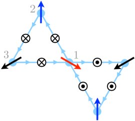
Figure 2: (Color online) Directions of the out-of-plane DM vectors. Arrows on the bonds show the ordering of the ${\bf S}_{i}$ and ${\bf S}_{j}$ operators in the vector-product in (27).

The antisymmetric Dzyaloshinskii-Moriya interaction is generally written as

$$\delta\hat{\cal H}_{DM}=\sum_{\langle ij\rangle}{\bf D}_{ij}\cdot({\bf S}_{i}\times{\bf S}_{j})\,.$$ (27)

In order to determine the DM vectors ${\bf D}_{ij}$ one has to specify the order of sites in the vector product, which may be represented by the bond direction from the first to the second spin in each pair. A convenient choice consists of ordering spins uniformly along the chains, see Fig. 2. Then, the symmetry analysis yields a unique pattern of the DM vectors orthogonal to the kagomé plane as shown in Fig. 2. Elhajal02 ; Cepas08 ; Sachdev10 Note, that the in-plane components of the DM vectors are strictly forbidden once the the kagomé plane coincides with a mirror crystal plane. Elhajal02

Apparent alternation of the DM vectors between up triangles with ${\bf D}_{ij}\!=\!(0,0,-D_{z})$ and down triangles with ${\bf D}_{ij}\!=\!(0,0,D_{z})$ is partly fictitious, because it is a consequence of the chosen bond gauge, in which the two types of triangles are circumvented oppositely, Fig. 2. The DM interactions on the two triangles favor the same sense of spin rotation or chirality. Hence, for a given sign of $D_{z}$, the DM term (27) selects one of the two ${\bf q}\!=\!0$ structures with positive ($D_{z}\!>\!0$) or negative ($D_{z}\!<\!0$) chiralities, yielding energy gain $E_{\rm cl}\!=\!-\sqrt{3}|D_{z}|S^{2}$ per site. On the other hand, for the $\sqrt{3}\times\!\sqrt{3}$ state contributions from up and down triangles come with opposite sign and cancel out. In the following, we assume $D_{z}\!>\!0$ and, consequently, perform the spin-wave expansion around the ${\bf q}\!=\!0$ state with positive chiralities, see Fig. 2. It is also straightforward to see that the DM term does not induce additional canting and preserves the 120^∘ magnetic structure in the $x$–$y$ plane.

Consider the DM term (27) on the $(1,2)$ bond in Fig. 2 written in the rotating local spin basis (2)

$$\hat{\cal H}^{(1,2)} = D_{z}\sin\theta_{12}\left(S_{2}^{z}S_{1}^{z}+S_{2}^{x}S_{1}^{x}\right)$$ (28)

$$+D_{z}\cos\theta_{12}\left(S_{2}^{z}S_{1}^{x}-S_{2}^{x}S_{1}^{z}\right)\,,$$

where $\theta_{ij}\!=\!\theta_{i}\!-\!\theta_{j}$, and the first term contributes to the classical, harmonic, and quartic orders of the $1/S$ expansion, while the second contributes in the cubic order.

Since the DM term concerns only the nearest-neighbor pairs of spins and because in the ${\bf q}\!=\!0$ state all DM bonds contribute identically, the overall structure of the harmonic part of the Hamiltonian remains the same as in (9). Then, some algebra yields the harmonic Hamiltonian $\hat{\cal H}_{2}$ in the form (13) with the DM contributions

$$\delta\hat{\bf A}_{\bf k}=d_{M}\left(\hat{\bf I}-\frac{1}{4}\,\hat{\bm{\Lambda}}_{\bf k}\right),\ \ \ \delta\hat{\bf B}_{\bf k}=\frac{d_{M}}{4}\,\hat{\bm{\Lambda}}_{\bf k}\,,$$ (29)

where $d_{M}\!=\!\sqrt{3}D_{z}/J$ and $\hat{\bm{\Lambda}}_{\bf k}$ is unchanged from (10), again reducing the eigenvalue problem of the harmonic spin-wave theory to the one of $\hat{\bm{\Lambda}}_{\bf k}$, already solved in (17) and (18). Then, the spin-wave frequencies for the problem with the out-of-plane DM interaction (27) are $\omega_{\nu,\bf k}=\sqrt{\left(1+d_{M}\right)\left(1-\lambda_{\nu,\bf k}/2\right)\left(1+d_{M}+\lambda_{\nu,\bf k}\right)}$. With $\lambda_{\nu,\bf k}$ from (18), the flat mode energy is

$$\varepsilon_{1,\bf k}=2JS\sqrt{3d_{M}\left(1+d_{M}\right)/2}\,,$$ (30)

and the energies of the dispersive modes are

$$\varepsilon_{2(3),\bf k}=2JS\sqrt{1+d_{M}}$$ (31)

$$\phantom{\varepsilon_{2(3),\bf k}}\times\sqrt{1+d_{M}-\gamma_{\bf k}-d_{M}\bigl{(}1\pm\sqrt{1+8\gamma_{\bf k}}\,\bigr{)}/4}\,,\ \ \ \$$

which are similar to the $XXZ$ (22) and the single-ion (25), (26) results and are in agreement with Ref. Yildirim06, . The energies of the magnon modes $\varepsilon_{\nu,\bf k}$ are illustrated in Fig. 3 for the DM term $D_{z}/J\!=\!0.06$, a value relevant to the Fe-jarosite.Matan06 ; Yildirim06

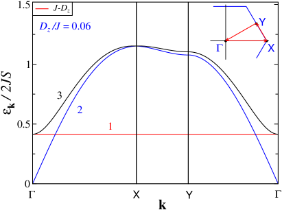
Figure 3: (Color online) Energies of the three magnon modes for the $J$–$D_{z}$ spin model with the out-of-plane DM interaction $D_{z}/J=0.06$ along a representative path in the Brillouin zone.

Opposite to the previous extensions, the DM term contributes to the cubic anharmonicities, see (28). Using the second term in (28) for one bond and extending it to the entire lattice we find for the ${\bf q}\!=\!0$ state

$$\hat{\cal H}_{3}=\frac{d_{M}}{3}\,J\sqrt{\frac{S}{2}}\sum_{i,j}\sin\theta_{ij}\bigl{(}a_{i}^{\dagger}a_{j}^{\dagger}a^{\phantom{{\dagger}}}_{j}+\textrm{h.c.}\bigr{)}\,,$$ (32)

whose structure is identical to the cubic term from the $J$-part of the Hamiltonian (47) considered in Sec. III. Thus, the out-of-plane DM interaction in the ${\bf q}\!=\!0$ state simply renormalizes cubic vertices by a factor $(1+d_{M}/3)$.

II.6 Small-$J_{2}$ expansion

In the Heisenberg kagomé-lattice antiferromagnet, additional next-nearest-neighbor coupling $J_{2}$ lifts the degeneracy of the 120^∘ manifold of classical states and selects between the ${\bf q}\!=\!0$ and $\sqrt{3}\times\!\sqrt{3}$ ground states.Harris92 ; Chubukov92 It also introduces a dispersion into the “flat mode” energy and thus was invoked to reproduce experimentally observed ${\bf k}$-dependence of such mode in Fe-jarosite.Yildirim06 We note, however, that quantum fluctuations beyond the harmonic order also generate effective $J_{2}$ interactions,Chubukov92 ; ChZh14 and thus could be the source of the same ${\bf k}$-dependence. As we show in Sec. III, the dispersion of the flat mode is particularly important for the quasi-resonant spin-wave decays. Below, we consider the effect of small $J_{2}$ perturbatively. Other types of small interactions can be taken into account in a similar fashion.

We first point out that the network of the second-neighbor bonds forms three independent kagomé lattices. Second, these bonds connect only spins from different sublattices of the original lattice, see Fig. 1. Therefore, contribution of the $J_{2}$ term to the harmonic spin-wave Hamiltonian has the same structure as the nearest-neighbor Hamiltonian (9)

$$\delta\hat{\cal H}^{\prime}_{2} = 2J_{2}S\sum_{{\bf k},\alpha\beta}\biggl{\{}\Bigl{[}\delta_{\alpha\beta}+\frac{1}{4}\,\Lambda^{\prime\,\alpha\beta}_{\bf k}\Bigr{]}a_{\alpha,\bf k}^{\dagger}a^{\phantom{{\dagger}}}_{\beta,\bf k}$$ (33)

$$\phantom{2J_{2}S}-\frac{3}{8}\,\Lambda^{\prime\,\alpha\beta}_{\bf k}\bigl{(}a_{\alpha,\bf k}^{\dagger}a^{\dagger}_{\beta,-\bf k}+\textrm{h.c.}\bigr{)}\biggr{\}},$$

where instead of $\hat{\bm{\Lambda}}_{\bf k}$ the matrix is

$$\hat{\bm{\Lambda}}^{\prime}_{\bf k}=\left(\begin{array}[]{ccc}0&c^{\prime}_{3}&c^{\prime}_{1}\\ c^{\prime}_{3}&0&c^{\prime}_{2}\\ c^{\prime}_{1}&c^{\prime}_{2}&0\end{array}\right)\,,$$ (34)

and we use the shorthand notations $c^{\prime}_{1}\!=\!\cos(q_{3}\!+\!q_{2})$, $c^{\prime}_{2}\!=\!\cos(q_{3}\!-\!q_{1})$, $c^{\prime}_{3}\!=\!\cos(q_{1}\!+\!q_{2})$ with $q_{n}\!=\!{\bf k}\cdot\bm{\delta}_{n}/2$.

Therefore, the diagonalization of the harmonic part of the $J-J_{2}$ Hamiltonian requires diagonalization of the matrix $\widetilde{\bm{\Lambda}}_{\bf k}\!=\!\hat{\bm{\Lambda}}_{\bf k}+j_{2}\hat{\bm{\Lambda}}^{\prime}_{\bf k}$, where $j_{2}\!=\!J_{2}/J$. Generally, this can be done numerically, the approach taken in Ref. Yildirim06, in the analysis of the Fe-jarosite spectrum, with the analytical results given only for the high-symmetry points. However, having in mind the problem of spin-wave excitation in large-$S$ kagomé-lattice antiferromagnet, for the physical range of interest $J_{2}\!\ll\!J$ one can make analytical progress using an expansion in $j_{2}$.

Figure 4: (Color online) Evolution of the “flat mode” upon switching on additional interactions with parameters shown in the legend. Solid lines: energies of the “flat mode” for the $J-J_{2}$ Heisenberg (lower curve) and out-of-plane DM models (upper curve), using approximate expressions in Eqs. (37) and (II.6). Dashed lines are the energies for the same models at $J_{2}=0$. Dotted lines (virtually indistinguishable from solid lines) are exact results, without using the expansion in $J_{2}$.

Because the most important qualitative effect of $J_{2}$ is the dispersion of the flat band, we will ignore small corrections to the “normal” modes. Expanding characteristic equation for the matrix $\widetilde{\bm{\Lambda}}_{\bf k}$ in $j_{2}$ we obtain

$$\left(\lambda+1\right)\left(\lambda^{2}-\lambda-2\gamma_{\bf k}\right)=2j_{2}\left(\lambda f_{1}({\bf k})+f_{2}({\bf k})\right),\ \ \$$ (35)

$$\mbox{where}\ \ \ f_{1}({\bf k})=c_{1}^{\prime}c_{1}+c_{2}^{\prime}c_{2}+c_{3}^{\prime}c_{3}\,,$$

$$\phantom{\mbox{where}\ \ \ }f_{2}({\bf k})=c_{1}^{\prime}c_{2}c_{3}+c_{2}^{\prime}c_{1}c_{3}+c_{3}^{\prime}c_{1}c_{2}\,.$$

Then, the “flat mode” $\lambda_{1}\!=\!-1$ eigenvalue is modified as

$$\widetilde{\lambda}_{1,{\bf k}}=\lambda_{1}+j_{2}\lambda^{(1)}_{1,{\bf k}}\,,\ \ \lambda^{(1)}_{1,{\bf k}}=\left(\frac{f_{2}({\bf k})-f_{1}({\bf k})}{1-\gamma_{\bf k}}\right)\,.$$ (36)

Corrections to $\lambda_{2}$ and $\lambda_{3}$ can be obtained similarly.

Having this perturbative correction to $\lambda_{1}$ in (36) allows us to obtain the flat mode energies in various models. We list some of the answers below.

(i) $J-J_{2}$ Heisenberg model:

$$\varepsilon_{1,\bf k}=2JS\sqrt{3j_{2}(1+\lambda^{(1)}_{1,{\bf k}})/2}+{\cal O}(j_{2}^{3/2})\,.$$ (37)

(ii) $J-J_{2}$ $XXZ$ model. Here we assume that the anisotropy $\Delta$ is the same in both exchanges:

$$\varepsilon_{1,\bf k} = 2JS\sqrt{3/2+j_{2}(1-\lambda^{(1)}_{1,{\bf k}}/2)}$$

$$\times\sqrt{1-\Delta+j_{2}(1+\lambda^{(1)}_{1,{\bf k}})}+{\cal O}(j_{2}^{2})\,.$$

(iii) $J-J_{2}$ out-of-plane DM model.

$$\varepsilon_{1,\bf k} = 2JS\sqrt{3(1+d_{M})/2+j_{2}(1-\lambda^{(1)}_{1,{\bf k}}/2)}\ \ \$$

$$\times\sqrt{d_{M}+j_{2}(1+\lambda^{(1)}_{1,{\bf k}})}+{\cal O}(j_{2}^{2})\,,$$

where $d_{M}\!=\!\sqrt{3}D_{z}/J$ as before. This is the model which was used to describe the spectrum of Fe-jarosite.Yildirim06 Our results agree exactly with the expressions for the high-symmetry points provided in Ref. Yildirim06, . The advantage of our approach is that it is fully analytical in the entire Brillouin zone.

Effects of the second-neighbor exchange $J_{2}$ and the DM coupling $D_{z}$ on the dispersion of the “flat mode” $\varepsilon_{1,\bf k}$ are summarized in Fig. 4 for representative values $J_{2}/J\!=\!0.03$ and $D_{z}/J\!=\!0.06$ that are motivated by the experimental data for Fe-jarosite; Matan06 ; Yildirim06 the $J_{2}\!=\!0$ energies are also shown. In the same figure the energies obtained via numerical diagonalization of the matrix $\widetilde{\bm{\Lambda}}_{\bf k}$ are shown. The corresponding results are indistinguishable from the approximate results of Eqs. (37) and (II.6) on the scale of our plot.

II.7 Two-step diagonalization

For the above three cases, the $XXZ$, the single-ion, and the out-of-plane DM models, the harmonic spin-wave theory includes diagonalization of the same matrix $\hat{\bm{\Lambda}}_{\bf k}$. Here we elaborate on details of this general procedure and provide the formalism, which is essential for treating the non-linear terms in all these models and is identical for all considered cases.

Following Ref. Harris92, , diagonalization of $\hat{\bm{\Lambda}}_{\bf k}$ implies a two-step diagonalization procedure of $\hat{\cal H}_{2}$ in the form (13). Its eigenvectors ${\bf w}^{\dagger}_{\nu}=\left(w_{\nu,1}({\bf k}),w_{\nu,2}({\bf k}),w_{\nu,3}({\bf k})\right)$ obey

$$\hat{\bm{\Lambda}}_{\bf k}{\bf w}_{\nu}=\lambda_{\nu,\bf k}{\bf w}_{\nu}$$ (40)

and can be found explicitlyHarris92 ; ChZh14

$${\bf w}_{\nu}({\bf k})=\frac{1}{r_{\nu}}\,\left(\begin{array}[]{c}c_{1}c_{2}+\lambda_{\nu}c_{3}\\ \lambda_{\nu}^{2}-c_{1}^{2}\\ c_{1}c_{3}+\lambda_{\nu}c_{2}\end{array}\right)\,,$$ (41)

with $r_{\nu}=\sqrt{(c_{1}c_{2}+\lambda_{\nu}c_{3})^{2}\!+(\lambda_{\nu}^{2}-c_{1}^{2})^{2}\!+(c_{1}c_{3}\!+\lambda_{\nu}c_{2})^{2}}$.

These eigenvectors define a unitary transformation of the original Holstein-Primakoff bosons to the new ones

$$a^{\phantom{{\dagger}}}_{\alpha,\bf k}=\sum_{\nu}w_{\nu,\alpha}({\bf k})\,d^{\phantom{{\dagger}}}_{\nu,\bf k}\,,\ \ d^{\phantom{{\dagger}}}_{\nu,\bf k}=\sum_{\alpha}w_{\nu,\alpha}({\bf k})\,a^{\phantom{{\dagger}}}_{\alpha,\bf k}\,,$$ (42)

such that the harmonic Hamiltonian $\hat{\cal H}_{2}$ in the form of (9) with $\hat{\bf A}_{\bf k}$’s and $\hat{\bf B}_{\bf k}$’s from (14) with (21), (24), or (29) is turned into three independent Hamiltonians

$$\hat{\cal H}_{2}=2JS\sum_{\nu,\bf k}\Bigl{[}A_{\nu,\bf k}d_{\nu,\bf k}^{\dagger}d^{\phantom{{\dagger}}}_{\nu,\bf k}-\frac{B_{\nu,\bf k}}{2}\bigl{(}d^{\dagger}_{\nu,\bf k}d^{\dagger}_{\nu,-\bf k}+\textrm{h.\,c.}\bigr{)}\Bigr{]}.$$

The final step is the conventional Bogolyubov transformation for each individual species of the $d$-bosons

$$d^{\phantom{{\dagger}}}_{\nu,\bf k}=u_{\nu\bf k}b^{\phantom{{\dagger}}}_{\nu,\bf k}+v_{\nu\bf k}b^{\dagger}_{\nu,-\bf k}\,,$$ (43)

with $u_{\nu\bf k}^{2}-v_{\nu\bf k}^{2}=1$ and

$$v_{\nu\bf k}^{2}=\frac{1}{2}\Bigl{(}\frac{A_{\nu,\bf k}}{\omega_{\nu,\bf k}}-1\Bigr{)},\quad 2u_{\nu\bf k}v_{\nu\bf k}=\frac{B_{\nu,\bf k}}{\omega_{\nu,\bf k}}\,,$$ (44)

where the eigenvalues $\omega_{{\nu,\bf k}}$, $A_{\nu,\bf k}$, and $B_{\nu,\bf k}$ were obtained for each of the models in previous sections. The importance of this two-step procedure will be apparent in the discussions of the non-linear terms in Sec. III.

II.8 Ordered magnetic moment

Here we discuss the dependence of the ordered magnetic moment on anisotropy parameter and on the value of the spin $S$. While we only consider the $XXZ$ model,ChZh14 the results are expected to be similar for the other anisotropies considered above. It should be noted that this calculation can only qualitatively estimate the stability of the Neél order, because it only includes the “diagonal” quantum fluctuation for a given state, completely neglecting the “off-diagonal” tunneling processes between different states within the manifold. On the other hand, such processes should be exponentially suppressed for larger spins. Henley93

Within the linear spin-wave theory, magnetic moment on a site that belongs to the sublattice $\alpha$ is reduced by zero-point fluctuations: $\langle S\rangle_{\alpha}=S-\langle a_{\alpha,\ell}^{\dagger}a^{\phantom{{\dagger}}}_{\alpha,\ell}\rangle$. Converting $a_{\alpha}$ to $d_{\mu}$ and then to $b_{\mu}$ using unitary (42) and Bogolyubov (43) transformations one arrives to

$$\langle S\rangle_{\alpha}=S-\frac{1}{N}\sum_{\mu,{\bf k}}w^{2}_{\mu,\alpha}({\bf k})\,v^{2}_{\mu{\bf k}}\,.$$ (45)

Since all three sublattices are equivalent, symmetrization of (45) gives

$$\langle S\rangle=S-\frac{1}{3N}\sum_{\mu,{\bf k}}v^{2}_{\mu{\bf k}}\,,$$ (46)

with $v^{2}_{\mu{\bf k}}$ from (44). Calculations of the magnetization $M\!=\!\langle S\rangle/S$ and the $\langle S\rangle\!=\!0$ Neél order boundary in the $S\!-\!\Delta$ plane are performed taking the 2D integrals in (46) numerically using (44) for the $XXZ$ model.

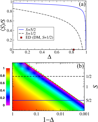
Figure 5: (Color online) (a) Magnetization $M\!=\!\langle S\rangle/S$ vs $\Delta$ for $S\!=\!1/2$ and $S\!=\!5/2$. Square is the ED result for $S\!=\!1/2$ with the DM interaction. (b) Intensity plot of the magnitude of $M$. Solid line is the $\langle S\rangle\!=\!0$ Neél order phase boundary in the $S\!-\!\Delta$ plane on the log-log scale, dashed line is the asymptotic approximation for it, see text.

Quantum suppression of the ordered moment vs anisotropy $\Delta$ is shown in Fig. 5(a) for two values of spin. Linear spin-wave theory suggests a disordered state near the Heisenberg limit for all spin values because quantum correction diverges for $\Delta\to 1$ due to vanishing energy of the “flat mode.” The critical value $1\!-\!\Delta_{c}\!\approx\!0.047$ for $S\!=\!1/2$ is compared in Fig. 5(a) with the result for the DM coupling $D_{z,c}\!=\!0.1$ (rescaling $1\!-\!\Delta_{c}\!\Leftrightarrow\!\sqrt{3}D_{z,c}$), found by exact diagonalization (ED). Cepas08 ; Messio10 Since the DM term suppresses tunneling processes within the manifold, it is reasonable to compare ED with spin-wave theory results to evaluate the accuracy of the Neél order boundary. One can see a qualitative agreement with ED and a quantitative exaggeration of the extent of the ordered phase, expected for the spin-wave approach.

Near the Heisenberg limit, one can neglect non-divergent terms in (46) and find an asymptotic expression for the Neél order boundary from $\langle S\rangle\!=\!0\!\approx\!S\!-\!A_{1}/6\omega_{1}$, where $A_{1}=3/4$, see (16), and $\omega_{1}=\sqrt{3(1-\Delta)/2}$, see (22), leading to $1\!-\!\Delta_{c}\!\approx\!1/96S^{2}$, which is shown in Fig. 5(b) together with the result of the numerical integration in (46) and demonstrates an exceedingly close agreement with it.

III Non-linear Spin-wave theory

In Sec. II we have considered three anisotropic models of the kagomé-lattice antiferromagnets in the harmonic approximation and outlined the approach to taking into account other terms, such as further-neighbor exchanges, perturbatively. In this Section, we derive the nonlinear, cubic and quartic terms of the spin-wave $1/S$ expansion and then exemplify their role in the ground-state selection and in the spectral properties of the kagomé-lattice antiferromagnets using representative cases.

Below, we first obtain cubic and quartic terms of the spin-wave expansion to conclude the formal development of the theory. Then the cubic vertices for ${\bf q}\!=\!0$ and $\sqrt{3}\times\!\sqrt{3}$ states allow us to proceed with calculating order-by-disorder fluctuating corrections to their ground-state energies for the $XXZ$ and single-ion anisotropy models. Both models demonstrate a quantum phase transition between the ${\bf q}\!=\!0$ and the $\sqrt{3}\times\!\sqrt{3}$ states as a function of anisotropy parameter. Hence, both cases present rare examples of the quantum order-by-disorder favoring a different state from the one selected by thermal fluctuations, the latter choosing the $\sqrt{3}\times\!\sqrt{3}$ structure regardless of the anisotropy. Harris92 ; Reimers93 ; Henley09 ; Huse92 ; Korshunov02 ; Rzchowski97 ; ChZh14 ; Gotze15

We then proceed with a calculation of the decay-induced effects in the structure-factor ${\cal S}({\bf q},\omega)$ within the DM model with $J_{2}$. While this calculation is aimed at giving a detailed account of the spectral properties of a specific kagomé-lattice antiferromagnet described by this model, $S=5/2$ Fe-jarosite, the outlined scenario should be applicable to a wide variety of the other flat-band frustrated spin systems. Petrenko ; Matan14 ; Balents_honeycomb ; Georgii15 We also note that the structure factor ${\bf q}$-dependence allows to “filter out” spectral contributions of specific modes in the portions of the ${\bf q}$-space while highlighting the others; a useful phenomenon characteristic to the non-Bravais lattices.

III.1 Cubic terms

In the $XXZ$, single-ion anisotropy, and Heisenberg models, (2) with or without the anisotropies in (20) and (23), the terms that lead to the cubic anharmonic coupling of the spin waves are identical and originate from the $S_{i}^{x}S_{j}^{z}$ part of (2). These terms are also the only ones that are able to distinguish between different 120^∘ spin configurations in these models by virtue of containing $\sin\theta_{ij}\!=\!\pm\sqrt{3}/2$ for the clockwise or counterclockwise spin rotation. In the bosonic representation they yield

$$\hat{\cal H}_{3}=J\sqrt{\frac{S}{2}}\sum_{i,j}\sin\theta_{ij}\bigl{(}a_{i}^{\dagger}a_{j}^{\dagger}a_{j}+\textrm{h.c.}\bigr{)}\,,$$ (47)

where $\theta_{ij}=\theta_{i}-\theta_{j}$ is the angle between two neighboring spins as before. Clearly, the spin-wave interaction resulting from this term has different amplitude for different spin patterns. For the DM model, the DM term (27) also contributes to the cubic anharmonicity, but its structure for the ${\bf q}\!=\!0$ state is identical to (47), see (32), so it gives a simple change of the overall factor in the vertex $J\!\rightarrow\!J\!+\!D_{z}/\sqrt{3}$.

Using (47), we now detail the derivation of the cubic vertices for the main contenders for the ground state, the ${\bf q}\!=\!0$ and the $\sqrt{3}\times\!\sqrt{3}$ states. We begin with the ${\bf q}\!=\!0$ pattern, for which $\hat{\cal H}_{3}$ in (47) can be rewritten as

$$\hat{\cal H}_{3}=-J\sqrt{\frac{3S}{2N}}\sum_{\alpha\beta,\bf k,q}\epsilon^{\alpha\beta\gamma}\cos(q_{\beta\alpha})a^{\dagger}_{\alpha,\bf q}a^{\dagger}_{\beta,\bf k}a_{\beta,\bf p}+\textrm{h.\,c.},$$ (48)

where $\epsilon^{\alpha\beta\gamma}$ is the Levi-Civita antisymmetric tensor, ${\bf p}={\bf k}+{\bf q}$, $q_{\beta\alpha}={\bf q}\cdot\bm{\rho}_{\beta\alpha}$, and $\bm{\rho}_{\beta\alpha}=\bm{\rho}_{\beta}-\bm{\rho}_{\alpha}$.

The unitary transformation (42) in (48) yields

$$\hat{\cal H}_{3}=-J\sqrt{\frac{3S}{2N}}\sum_{\bf k,q}\sum_{\nu\mu\eta}F^{\nu\mu\eta}_{\bf qkp}\,d_{\nu,\bf q}^{\dagger}d_{\mu,\bf k}^{\dagger}d_{\eta,\bf p}+\textrm{h.c.},$$ (49)

where ${\bf p}={\bf k}+{\bf q}$ and the amplitude is

$$F^{\nu\mu\eta}_{\bf qkp}=\sum_{\alpha\beta}\epsilon^{\alpha\beta\gamma}\cos(q_{\beta\alpha})\,w_{\nu,\alpha}({\bf q})w_{\mu,\beta}({\bf k})w_{\eta,\beta}({\bf p}).$$ (50)

Finally, the Bogolyubov transformation (43) gives

$$\hat{\cal H}_{3}=\frac{1}{3!}\frac{1}{\sqrt{N}}\sum_{\bf k,q}\sum_{\nu\mu\eta}V^{\nu\mu\eta}_{\bf qkp}\,b_{\nu,\bf q}^{\dagger}b_{\mu,\bf k}^{\dagger}b^{\dagger}_{\eta,\bf-p}+\textrm{h.c.},\quad\quad$$ (51)

$$\phantom{\hat{\cal H}_{3}\ \ }+\frac{1}{2!}\frac{1}{\sqrt{N}}\sum_{\bf k,q}\sum_{\nu\mu\eta}\Phi^{\nu\mu\eta}_{\bf qk;p}\,b_{\nu,\bf q}^{\dagger}b_{\mu,\bf k}^{\dagger}b_{\eta,\bf p}+\textrm{h.c.},\ \ \ \ \$$ (52)

with the vertices for the “source” and the “decay” terms

$$V^{\nu\mu\eta}_{\bf qkp}=-J\sqrt{\frac{3S}{2}}\;\widetilde{V}^{\nu\mu\eta}_{\bf qkp}\,,\ \ \Phi^{\nu\mu\eta}_{\bf qk;p}=-J\sqrt{\frac{3S}{2}}\;\widetilde{\Phi}^{\nu\mu\eta}_{\bf qk;p}\,,$$ (53)

where the symmetrized dimensionless vertices are

$$\widetilde{V}^{\nu\mu\eta}_{\bf qkp} = F^{\nu\mu\eta}_{\bf qkp}(u_{\nu\bf q}+v_{\nu\bf q})(u_{\mu\bf k}v_{\eta\bf p}+v_{\mu\bf k}u_{\eta\bf p})$$

$$\mbox{}+F^{\mu\eta\nu}_{\bf kpq}(u_{\mu\bf k}+v_{\mu\bf k})(u_{\nu\bf p}v_{\eta\bf q}+v_{\nu\bf p}u_{\eta\bf q})\qquad$$

$$\mbox{}+F^{\eta\nu\mu}_{\bf pqk}(u_{\eta\bf p}+v_{\eta\bf p})(u_{\nu\bf q}v_{\mu\bf k}+v_{\nu\bf q}u_{\mu\bf k})\,,$$

and

$$\widetilde{\Phi}^{\nu\mu\eta}_{\bf qk;p} = F^{\nu\mu\eta}_{\bf qkp}(u_{\nu\bf q}+v_{\nu\bf q})(u_{\mu\bf k}u_{\eta\bf p}+v_{\mu\bf k}v_{\eta\bf p})$$

$$\mbox{}+F^{\mu\eta\nu}_{\bf kpq}(u_{\mu\bf k}+v_{\mu\bf k})(u_{\nu\bf p}u_{\eta\bf q}+v_{\nu\bf p}v_{\eta\bf q})\qquad$$

$$\mbox{}+F^{\eta\nu\mu}_{\bf pqk}(u_{\eta\bf p}+v_{\eta\bf p})(u_{\nu\bf q}v_{\mu\bf k}+v_{\nu\bf q}u_{\mu\bf k})\,,$$

where we have used the symmetry property $F^{\nu\mu\eta}_{\bf qkp}\!=\!F^{\nu\eta\mu}_{\bf qpk}$.

Repeating the same calculation for the $\sqrt{3}\times\sqrt{3}$ state we obtain identical expressions for the cubic spin-wave Hamiltonian and corresponding vertices, but with different amplitudes $F^{\nu\mu\eta}_{\bf qkp}$ expressed as

$$F^{\nu\mu\eta}_{\bf qkp}=i\sum_{\alpha\beta}\epsilon^{\alpha\beta\gamma}\sin(q_{\beta\alpha})\,w_{\nu,\alpha}({\bf q})w_{\mu,\beta}({\bf k})w_{\eta,\beta}({\bf p}).$$ (56)

Explicit expressions for the unitary transformation eigenvectors $w_{\nu,\alpha}({\bf q})$ of the matrix $\hat{\bm{\Lambda}}_{\bf k}$ and of the parameters of the Bogolyubov transformation are instrumental in deriving analytic expressions of the cubic anharmonic terms. We also note that for all models considered here, the functional form of the cubic vertices (III.1) and (III.1) is identical, with all the differences hidden in the expressions of the Bogolyubov parameters $u_{\mu{\bf k}}$ and $v_{\mu{\bf k}}$ from (44).

The role of the cubic terms in the ground-state selection and in the spectrum of the kagomé-lattice antiferromagnets is discussed below in Sec. III.3 and Sec. III.4.

III.2 Quartic terms

In the Holstein-Primakoff bosonic representation of spin models, quartic terms originate from the $S_{i}^{x}S_{j}^{x}$, $S_{i}^{y}S_{j}^{y}$, and $S_{i}^{z}S_{j}^{z}$ parts of the Hamiltonian. In the models considered here, quartic terms do not help to differentiate between different states of the 120^∘ manifold, but lead to the overall ground-state energy shift and to the Hartree-Fock corrections to the spin-wave energies. Because of the coplanar 120^∘ spin configuration, the formal expressions for these contribution show a close similarity to the ones for the triangular-lattice Heisenberg model, see Ref. triPRB09, . Therefore, we simply list the quartic parts of the Hamiltonians of the $XXZ$ model and the DM term together with the expressions for the ground-state energy shift in the former model and for the spin-wave energy correction for the latter model. Technical details are offered in Appendix A.

The quartic terms in the $XXZ$ model, (2) and (20), are

$$\hat{\cal H}_{4}=\frac{J}{2}\sum_{\langle ij\rangle}\>\biggl{(}\frac{2\Delta+1}{8}\bigl{(}(n_{i}+n_{j})a_{i}a_{j}+{\rm h.c.}\bigr{)}$$ (57)

$$\phantom{\hat{\cal H}_{4}=\frac{J}{2}}-\frac{2\Delta-1}{8}\>\bigl{(}a^{\dagger}_{j}(n_{i}+n_{j})a_{i}+{\rm h.c.}\bigr{)}-n_{i}n_{j}\biggr{)},$$

where $n_{i}=a^{\dagger}_{i}a_{i}$ and we omitted the $\alpha$ indices of the bosonic variables for brevity.

The quartic contribution from the DM term (27) is

$$\hat{\cal H}_{4,DM}=\frac{D_{z}\sqrt{3}}{2}\sum_{\langle ij\rangle}\>\biggl{(}\frac{1}{8}\bigl{(}(n_{i}+n_{j})a_{i}a_{j}+{\rm h.c.}\bigr{)}$$ (58)

$$\phantom{\hat{\cal H}_{4,DM}=\frac{D_{z}\sqrt{3}}{2}}+\frac{1}{8}\>\bigl{(}a^{\dagger}_{j}(n_{i}+n_{j})a_{i}+{\rm h.c.}\bigr{)}-n_{i}n_{j}\biggr{)}.$$

By means of the Hartree-Fock decouplingOguchi60 outlined in Appendix A, one can obtain contribution of the quartic terms to the $1/S$ series expansion of the ground-state energy of any non-collinear spin model

$$E=E_{\rm cl}+\delta E^{(2)}+\delta E^{(3)}+\delta E^{(4)},$$ (59)

where the first term is the classical energy of order ${\cal O}(S^{2})$, the second is the harmonic correction from $\hat{\cal H}_{2}$, ${\cal O}(S)$, and the last two are from the nonlinear cubic and quartic terms, both ${\cal O}(1)$. While we discuss the cubic part of this expression later, the classical and harmonic energy terms (per spin) of the series in (59) for the $XXZ$ model are

$$E_{\rm cl}+\delta E^{(2)}=-JS^{2}-JS\bigg{(}1-\frac{1}{3N}\sum_{\mu,{\bf k}}\omega_{\mu,{\bf k}}\bigg{)},$$ (60)

with the frequencies from (22). The quartic member of the series (59) for the same model is

$$\delta E_{4}=-J\Big{[}n^{2}+m^{2}+\bar{\Delta}^{2}$$ (61)

$$\ -(2\Delta+1)\Big{(}n\bar{\Delta}+\frac{m\delta}{2}\Big{)}+(2\Delta-1)\Big{(}nm+\frac{\bar{\Delta}\delta}{2}\Big{)}\Big{]},$$

where the Hartree-Fock averages are introduced in a standard manner

$$n=\langle a^{\dagger}_{i}a_{i}\rangle,\ \ m=\langle a^{\dagger}_{i}a_{j}\rangle,\ \ \bar{\Delta}=\langle a_{i}a_{j}\rangle,\ \ \delta=\langle a^{2}_{i}\rangle,$$ (62)

and are given in Appendix A.

In the same order of expansion, quartic terms lead to the Hartree-Fock corrections to the linear spin-wave Hamiltonian

$$\delta\hat{\cal H}_{2}=2J\sum_{\nu,\bf k}\delta A_{\nu,\bf k}d_{\nu,\bf k}^{\dagger}d^{\phantom{{\dagger}}}_{\nu,\bf k}-\frac{\delta B_{\nu,\bf k}}{2}\bigl{(}d^{\dagger}_{\nu,\bf k}d^{\dagger}_{\nu,-\bf k}+\textrm{h.\,c.}\bigr{)},$$

which yields the Hartree-Fock part of the $1/S$ contribution to the spin-wave energy

$$\varepsilon^{(4)}_{\nu,\bf k}=2J\>\frac{A_{\nu,\bf k}\delta A_{\nu,\bf k}-B_{\nu,\bf k}\delta B_{\nu,\bf k}}{\omega_{\nu,\bf k}}\,.$$ (63)

Here we give expressions for $\delta A_{\nu,\bf k}$ and $\delta B_{\nu,\bf k}$ for the Heisenberg model (2) with the DM anisotropy (27) as an example

$$\delta A_{\nu,\bf k}=\widetilde{C}_{1}+\frac{\widetilde{C}_{2}\lambda_{\nu,\bf k}}{2},\ \ \delta B_{\nu,\bf k}=-2\widetilde{C}_{4}-\frac{\widetilde{C}_{3}\lambda_{\nu,\bf k}}{2},$$ (64)

where $\widetilde{C}_{i}=C_{i}-d_{M}D_{i}$ and the constants are the linear combinations of the binary Hartree-Fock averages in (62) and can be found in Appendix A. We note that since the “flat-mode” eigenvalue $\lambda_{1,\bf k}=-1$, the quartic $1/S$ correction to its energy, $\varepsilon^{(4)}_{1,\bf k}$ in (63), is also necessarily momentum-independent in all models considered here. Therefore, it is a contribution of the cubic terms which is going to introduce a fluctuation-induced dispersion in the flat mode in the same order of the $1/S$ expansion.

III.3 Ground state selection

Here, we discuss the role of cubic terms (51) in the ground-state selection in the $XXZ$ and the single-ion anisotropy models. As was mentioned above, in the case of these models, (2) with (20) and (23), classical and harmonic terms are not able to lift the degeneracy in the manifold of coplanar 120^∘ structures. It is also easy to see from (2) that the quartic terms are also unable to differentiate between 120^∘ states, leaving the cubic term as a sole source of the quantum order-by-disorder effect to this order in $1/S$. The same is also true for the single-ion term in (23).

The second-order energy correction from the cubic terms (51) resulting in $\delta E^{(3)}$ in (59) is represented by the diagram in the lower inset of Fig. 6 and is given by

$$\delta E^{(3)}=-\frac{1}{18N^{2}}\sum_{\nu\mu\eta}\sum_{{\bf q},{\bf k}}\frac{|V^{\nu\mu\eta}_{{\bf q},{\bf k},-{\bf k}-{\bf q}}|^{2}}{\varepsilon_{\nu,\bf q}+\varepsilon_{\mu,\bf k}+\varepsilon_{\eta,-{\bf k}-{\bf q}}}\,,$$ (65)

where the energy is per spin and $N$ is the number of unit cells. Summation over magnon branches $\mu,\nu,\eta$ gives twenty seven individual contributions of which ten are distinct. With the formal expression for the source vertices in (III.1), the energy correction in (65) is identical for the $XXZ$ and the single-ion cases, with the differences in the expressions for the spin-wave energies $\varepsilon_{\alpha,\bf k}$ in (22) and (25) and (26), and in the $u_{\alpha\bf k}$ and $v_{\alpha\bf k}$ parameters (44) in vertices (III.1) for the corresponding models.

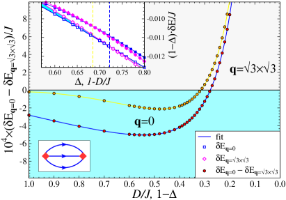
Figure 6: (Color online) Difference of the ground-state energies of the ${\bf q}\!=\!0$ and $\sqrt{3}\times\!\sqrt{3}$ states per spin. Upper inset: energy correction $\delta E^{(3)}$ for the ${\bf q}\!=\!0$ (squares) and $\sqrt{3}\times\!\sqrt{3}$ state (diamonds). Dashed vertical lines mark the transition. Upper data points/lines in the figure and inset are for the single-ion anisotropy model, (2) with (23), and the lower are for the $XXZ$ model, (2) with (20). Lower inset: diagram for $\delta E^{(3)}$ term (65) in the energy expansion (59).

Using an explicit form for the cubic vertices for the ${\bf q}\!=\!0$ and $\sqrt{3}\times\!\sqrt{3}$ spin states, we performed a high-accuracy numerical integration in Eq. (65) and studied the quantum order-by-disorder effect. Results of these calculations are presented in Fig. 6. The quantum selection of the ${\bf q}\!=\!0$ state over the $\sqrt{3}\times\!\sqrt{3}$ counterpart for the large planar anisotropy $(1-\Delta_{c})[D_{c}/J]\!\gtrsim\!0.3$ was highlighted in our previous work on the $XXZ$ model. ChZh14 This qualitative conclusion is in contrast with the usual behavior, in which quantum fluctuations lead to the same ground state that is selected by the thermal fluctuations. Indeed, for the classical kagomé-lattice antiferromagnets in both Heisenberg and $XY$ limits, thermal fluctuations select the $\sqrt{3}\times\!\sqrt{3}$ magnetic structure as the leading instability Harris92 ; Reimers93 ; Henley09 ; Huse92 ; Korshunov02 ; Rzchowski97 contrary to the behavior of the quantum model.

Here we complement the above result by the analysis of the single-ion anisotropy model (23). While the overall trend in $\delta E^{(3)}_{{\bf q}=0}-\delta E^{(3)}_{{\bf q}=\sqrt{3}\times\sqrt{3}}$ and, in particular, the transition point between the states in both models in Fig. 6 are very similar, there is a quantitative difference. As we have noted previously, the local real-space structure of the degeneracy-lifting terms is different in the $XXZ$ and single-ion models, implying a higher-order real-space path needed for generating the ground-state selection in the latter model.Zh_RSunpub Fig. 6 provides a strong support to this point, as the energy difference is smaller for the single-ion model by a factor $2-8$ for the range of $0.3\!<\!(1-\Delta)[D/J]\!<\!1$, in a qualitative agreement with the parameter of the real-space expansion being $\sim 1/z$ ($z=4$, coordination number). ChZh14

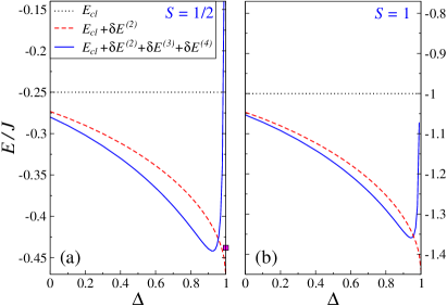
Figure 7: (Color online) Energy per site of the ${\bf q}\!=\!0$ state in the $XXZ$ model. Dotted line is for the classical term $E_{\rm cl}=-JS^{2}$, dashed is $E_{\rm cl}+\delta E^{(2)}$ in (60), and solid line is for (59) with $\delta E^{(3)}$ and $\delta E^{(4)}$ from (61) and (65). Square is the DMRG energy for the spin-liquid state.Yan11 (a) $S=1/2$, (b) $S=1$.

We conclude the discussion of the ground state with Fig. 7, which shows the energy of the ${\bf q}\!=\!0$ state in (59) vs $\Delta$ for the $XXZ$ model for two representative spin values $S\!=\!1/2$ and $S\!=\!1$. Classical and harmonic contributions to the ground-state energy are also indicated by dotted and dashed lines. Note that the energy difference shown in Fig. 6 would be nearly invisible on the scale of the plot in Fig. 7. We also note that although $\delta E^{(3)}$ and $\delta E^{(4)}$ from (61) and (65) represent the entire contribution of the ${\cal O}(1)$ order in the $1/S$ expansion of the ground-state energy (59), their divergences at $\Delta\rightarrow 1$ do not cancel completely, thus signifying a breakdown of the standard $1/S$ expansion at the Heisenberg limit because of the vanishing energy of the flat mode.Chubukov92

III.4 Spectrum and decays

We now turn to the spectral properties of the kagomé-lattice antiferromagnets. The goal of our consideration is twofold. First, we would like to highlight an unusual spectral property that has to be present in a wide variety of frustrated spin systems with excitations featuring flat branches.Ch15 Second, we give a detailed account of such spectral properties in a specific model that describes Fe-jarosite.Matan06 ; Yildirim06 Because of that we concentrate on the out-of-plane DM-anisotropy model, (2) with (27), of the $S\!=\!5/2$ nearest-neighbor kagomé-lattice antiferromagnet, which closely describes Fe-jarosite in the range of small $D_{z}$. One can expect the results of this consideration to be similar to the ones for the $XXZ$ and single-ion anisotropy models given the similarity of their harmonic spectra and anharmonic terms, even though the ground-state selection is more subtle in the later models.

III.4.1 Formalism and a qualitative discussion

Regardless of the model, using standard diagrammatic rules with the cubic terms in (51) and (52) produces the spin-wave self-energy in the form

$$\Sigma_{\mu,{\bf k}}(\omega) = \frac{1}{2N}\sum_{{\bf q},\nu\eta}\Bigg{(}\frac{|\Phi^{\nu\eta\mu}_{{\bf q},{\bf k}-{\bf q};{\bf k}}|^{2}}{\omega-\varepsilon_{\nu,\bf q}-\varepsilon_{\eta,{\bf k}-{\bf q}}+i\delta}$$

$$\phantom{\frac{1}{2}\sum_{{\bf q},\nu\eta}\Bigg{(}}-\frac{|V^{\nu\eta\mu}_{{\bf q},-{\bf k}-{\bf q},{\bf k}}|^{2}}{\omega+\varepsilon_{\nu,\bf q}+\varepsilon_{\eta,{\bf k}-{\bf q}}-i\delta}\Bigg{)},$$

where the first and the second terms are the decay and the source self-energies. Because of the summation over the magnon branches $\nu$ and $\eta$ in the decay and source loops, there are nine terms in the sum in (III.4.1), only six of which are distinct. Note that for the DM model one has to change $J\!\rightarrow\!J\!+\!D_{z}/\sqrt{3}$ in the vertices.

Taken on-shell, $\omega\!=\!\varepsilon_{\mu,{\bf k}}$, the self-energy (III.4.1) represents a strictly $1/S$ correction to the magnon energy from the cubic terms, $\Sigma_{\mu,{\bf k}}(\varepsilon_{\mu,{\bf k}})\!=\!O(S^{0})$. The other term of the same order in the $1/S$-expansion is from the quartic terms, $\varepsilon^{(4)}_{\nu,\bf k}$, which was obtained for the DM model in (63). Then, the magnon Green’s function for the branch $\mu$ can be written as

$$G^{-1}_{\mu}({\bf k},\omega)=\omega-\varepsilon_{\mu,{\bf k}}-\varepsilon^{(4)}_{\mu,\bf k}-\Sigma_{\mu,{\bf k}}(\omega)\,,$$ (67)

which, generally, allows to evaluate the spectral function $A_{\mu}({\bf k},\omega)=-(1/\pi){\rm Im}G_{\mu}({\bf k},\omega)$ of the corresponding spin-wave branch $\mu$.

Since we are interested in the large-$S$ limit and in the resonance-like decay phenomenon in the spectrum, the following simplification can be used. Given the off-resonance character of the source term, the frequency-independence of the quartic terms, and the large-$S$ limit of the problem, one can neglect the real part of the $1/S$ corrections to the spectrum as a first step, and approximate the self-energy in (III.4.1) by its on-shell imaginary part, i.e. $\Sigma_{\mu}({\bf k},\omega)\!\approx\!i{\rm Im}\Sigma_{\mu}({\bf k},\varepsilon_{\mu,{\bf k}})\!=\!-i\Gamma_{\mu,{\bf k}}$, with

$$\Gamma_{\mu,{\bf k}}=\frac{\pi}{2N}\sum_{{\bf q},\nu\eta}|\Phi^{\nu\eta\mu}_{{\bf q},{\bf k}-{\bf q};{\bf k}}|^{2}\delta\left(\varepsilon_{\mu,\bf k}-\varepsilon_{\nu,\bf q}-\varepsilon_{\eta,{\bf k}-{\bf q}}\right),$$ (68)

where the summation is over magnon branches of the decay products. Using the dimensionless vertices in (III.1) and frequencies in (30) and (31), one can rewrite (68) as

$$\frac{\Gamma_{\mu,{\bf k}}}{J}=\frac{3\pi}{8N}\sum_{{\bf q},\nu\eta}|\widetilde{\Phi}^{\nu\eta\mu}_{{\bf q},{\bf k}-{\bf q};{\bf k}}|^{2}\delta\left(\omega_{\mu,\bf k}-\omega_{\nu,\bf q}-\omega_{\eta,{\bf k}-{\bf q}}\right),$$ (69)

which is explicitly independent of the spin value $S$. As is mentioned above, the summation over magnon branches in (69) contains six distinct terms, or potential “decay channels.” A particular decay channel may or may not be contributing to the decays, depending on the kinematic conditions discussed below.

Before we divert our attention to a specific model, the following qualitative consideration can be made. The form in (69) suggests that $\Gamma_{\mu,{\bf k}}={\cal O}(J)$, which is small compared to $\varepsilon_{\mu,\bf k}={\cal O}(JS)$ in the large-$S$ limit. Thus, generally, one can expect a regular, perturbative $1/S$-effect of broadening of the higher-energy part of the dispersive branches due to decays into the lower-energy states.RMP13 However, a spectacular exception to this rule must occur if both of the decay products, branches $\nu$ and $\eta$, belong to flat modes with $\omega_{1}=const$. Clearly, this decay channel produces an essential singularity in $\Gamma_{\mu,{\bf k}}$ and $\Sigma_{\mu}({\bf k},\omega)$ at the energy equal to twice the flat mode energy, the effect that can be seen as a resonance-like decay. Therefore, a special care must be exercised in this case as any residual dispersion of the flat mode becomes crucial in regularizing such a singularity.

In fact, the way of removing this singularity is offered by the same $1/S$ fluctuations due to cubic terms, as the self-energy (III.4.1) also yields a dispersion for the flat mode. This can also be interpreted as a fluctuation-generated further-neighbor $J_{2}$ spin-spin interactions,Chubukov92 ; ChZh14 and such a dispersion of the flat mode has been observed in Fe-jarosite.Matan06 Still, this scenario implies that the fluctuation-induced flat-mode bandwidth, $W_{1}\propto{\cal O}(1)$, is of the order $1/S$ compared to the bandwidths of the normal dispersive modes, $W_{2(3)}\propto{\cal O}(S)$.

Introducing this $1/S$ dispersion for the flat modes in (69), suggests that the near-resonance decay-induced broadening of the dispersive mode within the energy window of the width $2W_{1}$ near $2\omega_{1}$ should now scale as $\Gamma_{\mu,{\bf k}}={\cal O}(JS)$. This is the same energy scale as the spin-wave dispersion itself without any obvious additional smallness. Therefore, our analysis implies a very strong broadening, likely eliminating spectral weight nearly completely from the respective energy range even when spin $S$ is large, providing an example of a spectacular quantum effect in an almost classical system.

Thus, in theory, as $S\rightarrow\infty$, we predict that an anomalous broadening and a wipe-out of the spectral weight should remain in the spectra of the flat-band frustrated systems, albeit in the energy window of order ${\cal O}(J)$ while the spectrum width grows as ${\cal O}(JS)$. In practice, we argue that such a spectacularly strong quantum effect, leading to the quasiparticle breakdown with characteristic termination points and ranges of energies dominated by broad continua, must be present in an almost classical $S\!=\!5/2$ kagomé-lattice Fe-jarosite.

III.4.2 Decay channels in Fe-jarosite

An extensive analysis of the kinematic decay conditions in representative models of the frustrated spin systems has been provided previously.RMP13 ; triPRB09 Here, the modification of the problem is in having three different magnon branches, which modifies these condition to

$$\omega_{\mu,\bf k}=\omega_{\nu,\bf q}+\omega_{\eta,{\bf k}-{\bf q}}\,,$$ (70)

so that every decay channel $\mu\!\rightarrow\!\{\nu,\eta\}$ has to be analyzed separately. That is, for each branch $\mu$ up to six channels can be contributing independently to the decay rate

$$\Gamma_{\mu,{\bf k}}=\sum_{\{\nu,\eta\}}\Gamma_{{\bf k},\mu\rightarrow\{\nu,\eta\}}\,.$$ (71)

While the decay conditions are model-specific, Fe-jarosite offers a commonplace scenario: a predominantly nearest-neighbor Heisenberg system with subleading symmetry-breaking anisotropic term, which is responsible for lifting the flat mode to a finite energy. We, therefore, analyze the decay channels for this representative situation for a small $D_{z}=0.06J$, used in fitting spin-wave spectrum of Fe-jarosite.Yildirim06 The harmonic dispersions for this value of $D_{z}$ are shown in Fig. 4 and in the inset of Fig. 8(a), and we use them in our analysis.

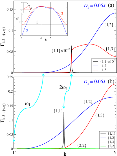
Figure 8: (Color online) Individual contributions to the decay rate in (69) from the decay channels $\Gamma_{{\bf k},\mu\rightarrow\{\nu,\eta\}}$ in units of $J$, (a) for mode 2, (b) for mode 3 in for the DM model. $D_{z}\!=\!0.06J$, ${\bf k}$ is along the $\Gamma$Y direction, and artificial broadening $\delta\!=\!0.002$ has been used. ${\bf k}$-values that correspond to $\omega_{1}$ and $2\omega_{1}$ are indicated by the arrows. Results for the “resonant” decay channel $2\!\rightarrow\!\{1,1\}$ are scaled down by the factor $10^{-2}$. Inset: harmonic frequencies $\omega_{\alpha,\bf k}$ along the representative cuts of the BZ for all three modes from Fig. 4.

We use the same numeration of the branches as before: 1=flat mode, 2=gapless mode (Goldstone branch), and 3=gapped dispersing mode. While the flat mode does have one active decay channel into two Goldstone modes, $1\!\rightarrow\!\{2,2\}$, for a small range of momenta near the center of the Brillouin zone, ${\bf k}\!<\!{\bf k}_{c}$ where ${\bf k}_{c}$ is the intersect point of the branches, see Fig. 8(a), its effect is truly minor and the main interest is in the decays of the dispersive modes. From the picture of harmonic energies, it is easy to see that the energy conservation in (70) can be satisfied for three (four) decay channels out of the six for the mode 2(3), one being the “resonance-like,” $2(3)\!\rightarrow\!\{1,1\}$, mentioned above, and two (three) are “regular.” The latter are $2(3)\!\rightarrow\!\{1,2\}$ and $2(3)\!\rightarrow\!\{1,3\}$, with an additional channel for the mode $3\!\rightarrow\!\{2,2\}$.

Using (69), we calculate contributions of the individual decay channels, $\Gamma_{{\bf k},\mu\rightarrow\{\nu,\eta\}}$, shown in Figs. 8(a) and (b), for modes 2 and 3 and for a representative ${\bf k}$-cut of the Brillouin zone. One can see that for $2(3)\!\rightarrow\!\{1,1\}$ it gives a $\delta$-peak at $2\omega_{1}$, that $2(3)\!\rightarrow\!\{1,2\}$ channel has a threshold at $\omega_{1}$ and $2(3)\!\rightarrow\!\{1,3\}$ at $2\omega_{1}$. In Fig. 8(a), the resonance decay rate is scaled down by $10^{-2}$ and would otherwise dwarf the rest even for the small artificial broadening of the $\delta$-function in (69).

A somewhat unexpected finding is a strong suppression of the $3\!\rightarrow\!\{2,2\}$ and the $3\!\rightarrow\!\{1,1\}$ channels. A closer analysis have identified different origins for them. For the $3\!\rightarrow\!\{2,2\}$ channel, decay products involve long-wavelength excitations from the Goldstone branch, which provides an extra smallness in the decay amplitude compared with the “regular” ones. For the $3\!\rightarrow\!\{1,1\}$ channel the situation is more subtle. One can demonstrate that the vertex $\widetilde{\Phi}^{113}_{\bf q,k-q;k}$ carries an extra $D_{z}$ compared with the vertex for the $2\!\rightarrow\!\{1,1\}$ channel, yielding a factor of about $1/100$ in the decay rate. The physical reason for this suppression can be hypothesized. Quasiclassically, the mode 2 is the “in-plane” mode, while modes 3 and 1 are “out-of-plane.” Then the in-plane mode can couple naturally to the two out-of-plane modes, while the out-of-plane mode has hard time splitting into two.

Thus, the suppression of the resonant decays of the mode 3 seems to be due to a subtle cancellation in the structure of the corresponding vertex. We note that for a realistic case of Fe-jarosite, other symmetry-breaking terms are also present, so one can expect the subtle cancellations of more symmetric models to be violated.

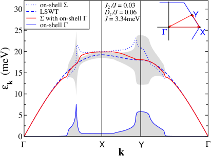
Figure 9: (Color online) Lower curve with the shading is the on-shell $\Gamma_{2,{\bf k}}$ from (69). Dashed line is the linear spin-wave theory energy of the gapless dispersive mode, $\varepsilon_{2,\bf k}$, from (31). Shaded area shows the half-width boundaries of a lorentzian peak, $\varepsilon_{2,\bf k}\pm\Gamma_{2,{\bf k}}$. Dotted and solid lines are different approximations for the renormalization of the real part of the self-energy in (III.4.1), see text. Parameters are as shown in the plot.

III.4.3 Spectrum of Fe-jarosite

We now finally approach the realistic description of the Fe-jarosite spectrum. We note that more details of this discussion is offered elsewhere.Ch15 As was mentioned above, the essential singularity in the dispersive modes is naturally removed by the residual dispersion of the flat mode. The experimentally observed dispersion of the flat modeMatan06 has been fitYildirim06 by introducing small next-nearest neighbor exchange $J_{2}=0.03J$, ignoring its possible quantum origin. Since we do not perform a fully self-consistent calculation here, the same approach suffices for the removal of the singularity in the decay rate (69). We, thus, modify the flat-mode dispersion according to (II.6) and ignore other corrections from the $J_{2}$ term.

In Sec. III.5 we elaborate on the possible way of separating contributions of different modes in the neutron-scattering structure factor, which allows us to concentrate on individual modes. Therefore, our Fig. 9 summarizes the effects of decays on the gapless dispersive mode only, as they are most pronounced in it. We have used parameters shown in the figure with the value of $J=3.34$meV from the previous work.Yildirim06

The lower curve shows the on-shell $\Gamma_{2,{\bf k}}$ obtained from (69) with the flat-mode dispersion from (II.6), and it includes all three decay channels discussed above. The dashed line is the linear spin-wave energy, $\varepsilon_{2,\bf k}$, with the shaded area around it representing $\varepsilon_{2,\bf k}\pm\Gamma_{2,{\bf k}}$, i.e., half-width at the half-maximum boundaries of a lorentzian peak. We have also taken into account renormalization of the real part of the self-energy in (III.4.1), with the dotted line showing the $1/S$ on-shell result and the solid line including effect of self-consistency by taking into account imaginary part from $\Gamma_{2,{\bf k}}$ in calculation of Re$\Sigma$. One can see that the resultant effects of the nonlinear terms on the real part of the spectrum are relatively minor, in agreement with the discussion after Eq. (67).

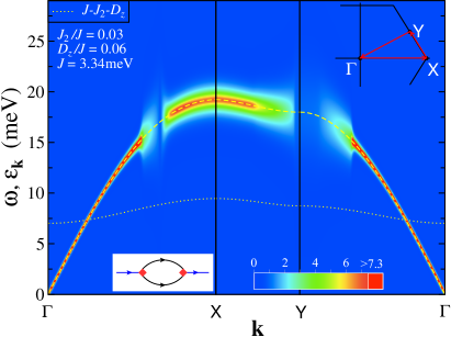
Figure 10: (Color online)  Intensity plot of the spectral function $A_{2}({\bf k},\omega)$ of the gapless mode in units of $(2SJ)^{-1}$ along the same path and for the same parameters as in Fig. 9, lines are from the same figure, see text. A small broadening $\delta/2SJ=0.002$ has been added to $\Gamma_{2,{\bf k}}$ in (68). Left panel inset: decay diagram.

We complement Fig. 9 by an intensity map of the spectral function, $A_{2}({\bf k},\omega)$, for the same dispersive mode along the same representative path in the Brillouin zone and for the same parameters, see Fig. 10. Dashed and dotted lines are the spin-wave results from Fig. 9 and are guides to the eye. The magnon self-energy is approximated by its on-shell imaginary part, as discussed above. The upper cut-off of the intensity of the spectral function corresponds to the maximal height of the peaks in the non-resonant decay region in Fig. 9 and translates into the broadening $\Gamma_{{\bf k}}\!\approx\!0.73$meV for the Fe-jarosite, easily resolvable by the modern neutron-scattering experiments.

Given the large spin value, $S=5/2$, we estimate that the ordered moment in Fe-jarosite should be nearly 90% of its classical value, see Fig. 5. It is then very natural to assume that the spectral properties should be fully describable by the harmonic spin-wave picture, the point of view taken in Ref. Yildirim06, . Indeed, our Figs. 9 and 10 demonstrate that the spin-wave excitation is sharp below the flat-band energy $\varepsilon_{1,{\bf k}}$ and acquires only an infinitesimal width for the energies above it. However, there is a sharp threshold at twice the bottom of the flat band minimum, $2\varepsilon^{\rm min}_{1,{\bf k}}$, above which there is a very strong broadening, reaching about one third of the bandwidth, signifying an overdamped spectrum.Ch15 Above $2\varepsilon^{\rm min}_{1,{\bf k}}$ in Fig. 10 there is a broad energy band with the features that look like a rip in the spectrum, consistent with the missing spectral weight in the experimental data. This threshold singularity is also remarkably similar to the spectral signatures of the quasiparticle breakdown phenomenon in quantum Bose liquids and $S=1/2$ spin-liquids. Zaliznyak ; Zheludev

Although at the energies above twice the top of the flat-band maximum, $2\varepsilon^{\rm max}_{1,{\bf k}}$, the decays are “regular,” i.e., occurring due to other, non-resonant channels, they are still providing a measurable broadening to the spectrum, so it is instructive to compare the two regions. The “regular” decays result in the maximal values of $\Gamma$ of order $0.2-0.3J$, an agreement with the similar effects in triangular-lattice antiferromagnetstriPRB09 and other frustrated spin systems.RMP13 The maximal broadening in the resonant-decay region is $\Gamma\approx 1.7J$ for the Fe-jarosite model, which is larger than the effect of the “regular” decays by a factor close to 5 ($=2S$). This is in a remarkably close accord with the qualitative argument on the scaling of the resonance decay rate with the spin value, provided after Eq. (69) above.

While a more detailed description of the spectral features of Fe-jarosite is given elsewhere,Ch15 we would like to highlight here a different, perhaps more dramatic view on the drastic transformations in its spectrum in the range of energies that falls within the resonant-decay band. In Fig. 11 we show an intensity plot of the constant-energy cut of the spectral function, $A_{2}({\bf k},\omega)$, of the same dispersive mode as in Figs. 9 and 10 for the energy 18meV, which is close to the middle of the resonant-decay region. The dashed lines show the expectations from the linear spin-wave theory of where the contours of sharp, well-defined peaks should have occurred. Instead, one can observe strong deviation from such expectations, characterized by a broadening, massive redistribution of the spectral weight into different regions of ${\bf k}$-space, together with the multitude of intriguing features, which are related to the van Hove singularities in the two-particle density of states of the flat-band decay products.triPRB09 Altogether, Figs. 9, 10, and 11 offer a convincing evidence of the highly non-trivial and very strong quantum effects in the the dynamical response of a nearly classical flat-band kagomé-lattice antiferromagnet, which are facilitated by the nonlinear couplings.

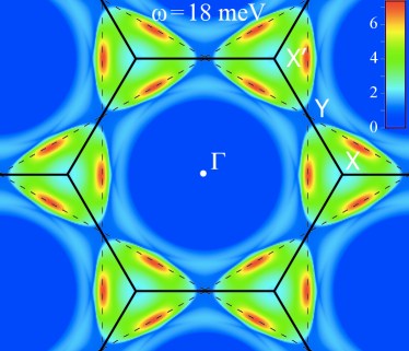
Figure 11: (Color online)  Intensity map of $A_{2}({\bf k},\omega)$ in units of $(2SJ)^{-1}$ vs ${\bf k}$ throughout the Brillouin zone for for the same set of parameters as in Fig. 9 for $\omega=18$meV. The upper cut-off of the intensity scale corresponds to the broadening $\Gamma_{2,{\bf k}}$ of 0.73 meV for the Fe-jarosite values of $S$ and $J$. Dashed black lines are peak positions from the linear spin-wave theory.

III.5 Dynamical structure factor

Inelastic neutron scattering cross-section is directly related to the diagonal components of the dynamical structure factor, or the spin-spin dynamical correlation function, given by

$${\cal S}^{i_{0}i_{0}}({\bf q},\omega)=\int_{-\infty}^{\infty}\frac{dt}{2\pi}\,e^{i\omega t}\langle S^{i_{0}}_{\bf q}(t)S^{i_{0}}_{-\bf q}\rangle\,,$$ (72)

where $i_{0}$ refers to the laboratory frame $\{x_{0},y_{0},z_{0}\}$ and

$$S^{i_{0}}_{\bf q}=\sum_{\alpha}S^{i_{0}}_{\alpha,{\bf q}},$$ (73)

involves summation over the spins $\alpha$ in the unit cell.

Because of the coplanar spin configuration in the considered kagomé-lattice antiferromagnets, transformation from the laboratory reference frame of $i_{0}$ to the local spin basis of (2) yields a mix of different diagonal and off-diagonal terms in the structure factor,Mourigal13 which conveniently separate into the in-plane and out-of-plane parts of ${\cal S}^{\rm tot}({\bf q},\omega)$. Assuming equal contribution of all three $i_{0}$ components to the neutron-scattering cross sectionMourigal13 and using the mapping of spins on bosons (6) allows one to perform a straightforward $1/S$ ranking of different contributions to the structure factor, in which the transverse components are, as usual, dominate the longitudinal and mixed terms.

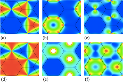
Figure 12: (Color online) Kinematic formfactors: $F^{\rm out}_{\nu\bf q}$ for the (a) flat, (b) dispersive gapless, (c) dispersive gapped mode; $F^{\rm in}_{\nu\bf q}$ for the (d) flat, (e) dispersive gapless, (f) dispersive gapped mode. $F^{\rm in}_{2\bf q}$ in (e) diverges at some $\Gamma$ points as $\omega^{-1}_{2,{\bf q}}$.

The subsequent algebra involves the two-step transformation (42) and (43) from the Holstein-Primakoff bosons to the quasiparticles, yielding the leading contributions to the structure factor as directly related to the spin-wave spectral functions $A_{\nu}({\bf q},\omega)$

$${\cal S}^{\rm in(out)}({\bf q},\omega)\approx\sum_{\nu}F^{\rm in(out)}_{\nu\bf q}A_{\nu}({\bf q},\omega)\,,$$ (74)

where we introduced kinematic formfactors

$$F^{\rm in}_{\nu\bf q}=\frac{S}{2}(u_{\nu\bf q}+v_{\nu\bf q})^{2}\left(1-R_{\nu{\bf q}}\right)\,,$$

$$F^{\rm out}_{\nu\bf q}=\frac{S}{2}(u_{\nu\bf q}-v_{\nu\bf q})^{2}\left(1+2R_{\nu{\bf q}}\right)\,,$$ (75)

with

$$R_{\nu{\bf q}}=\frac{1}{2}\sum_{\alpha\neq\alpha^{\prime}}w_{\nu,\alpha}({\bf q})w_{\nu,\alpha^{\prime}}({\bf q})\,.$$ (76)

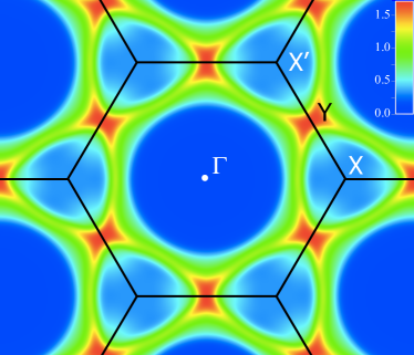
Figure 13: (Color online)  A 2D map of the inverse lifetime from (77) in units of $J$ in the ${\bf q}$-space. A small artificial gaussian ${\bf q}$-broadening with $\sigma=0.02\pi/a$ was used to mimic instrumental resolution. The scale is given in the inset and the maximal value of $\Gamma^{\rm max}_{2,{\bf q}}\approx 1.7J$ corresponds to about 6meV for Fe-jarosite.

An important property of the kinematic formfactors in (75) is their ${\bf q}$-dependence. They are modulated in the ${\bf q}$-space and are typically suppressed in one of the Brillouin zones while are maximal in the others. This effect is characteristic to the neutron-scattering in the non-Bravais lattices and is, in a way, similar to the effect known as the Bragg peak extinction for the elastic scattering in such lattices. Because of that property, one may be able to focus on a specific excitation branch without intermixing contributions from the others by selecting a particular component of the structure factor in a particular Brillouin zone.

Our Fig. 12 shows $F^{\rm in(out)}_{\nu\bf q}$ for three branches of excitations in the Fe-jarosite model. It demonstrates that such a “filtering out” can be quite useful. For example, the out-of plane component of the structure factor, ${\cal S}^{\rm out}({\bf q},\omega)$, should be dominated in one of the three distinct Brillouin zones by the spectral function $A_{2}({\bf q},\omega)$ of only one of the dispersive modes. This feature can be utilized in the neutron-scattering experiments.

Lastly, we highlight another quantitative way of analyzing ${\cal S}({\bf q},\omega)$. Assuming that one can focus on a particular excitation branch as mentioned above, one can suggest that a faithful representation of the inverse lifetime (linewidth) $\Gamma_{\mu{\bf q}}$ from (68) and its distribution in ${\bf q}$-space across the Brillouin zone can be obtained from the moments of the dynamical structure factor as Broholm

$$\widetilde{\Gamma}_{{\bf q}}=\sqrt{\langle\omega^{2}{\cal S}({\bf q},\omega)\rangle-\langle\omega{\cal S}({\bf q},\omega)\rangle^{2}},$$ (77)

where $\langle\omega^{n}{\cal S}({\bf q},\omega)\rangle\!=\!\int\omega^{n}{\cal S}({\bf q},\omega)d\omega$ are the moments of the structure factor and normalization $\langle{\cal S}({\bf q},\omega)\rangle\!=\!1$ is assumed. Then, this experimentally unbiased procedure would allow extracting a 2D ${\bf q}$-map of the quasiparticle broadening. We demonstrate the effectiveness of this approach in Fig. 13, which shows an example of such a map derived using the procedure in (77) from a gaussian form $A_{2}({\bf q},\omega)$, i.e. the gaussian function with a maximum at $\varepsilon_{2,{\bf q}}$ and the width $\Gamma_{2,{\bf q}}$. As expected, the extracted map of $\widetilde{\Gamma}_{{\bf q}}$ is nearly identical to the map of $\Gamma_{2,{\bf q}}$ itself. However, for a more natural lorentzian form of $A_{2}({\bf q},\omega)$ one can show that the extracted map corresponds to $\widetilde{\Gamma}_{{\bf q}}\!\propto\!\sqrt{\omega_{\rm max}\Gamma_{2,{\bf q}}}$, where $\omega_{\rm max}$ is the upper limit of the integration over $\omega$ in the moments in (77). Importantly, this result is still providing a direct information on the quasiparticle broadening map, albeit on a different scale. Therefore, aside from demonstrating at which momenta the decays are most intense, the suggested procedure also provides another way of “fingerprinting” of the broadening due to resonance-like decay into the flat modes.

IV Conclusions

In summary, we have provided a systematic consideration of the nonlinear $1/S$ expansion of several anisotropic models of the kagomé-lattice antiferromagnets. We have demonstrated the role of the nonlinear terms in the quantum order-by-disorder selection of the ground state and presented a strong evidence of the rare case of quantum and thermal fluctuations favoring different ground states in two of these models. We have provided a detailed analysis of the excitation spectrum of the $S=5/2$ iron-jarosite to illustrate our proposed general scenario of drastic transformations in the spectra of the flat-band frustrated magnets. Our study calls for further neutron-scattering experiments in these systems.

Appendix A Hartree-Fock corrections

The quartic terms in (57) yield a correction to the ground-state energy given by the four-boson averages, which are decoupled into the products of the binary Hartree-Fock averages (62) using Wick’s theorem

$$\langle a^{\dagger}_{i}a_{i}a^{\dagger}_{j}a_{j}\rangle=n^{2}+m^{2}+\bar{\Delta}^{2}\ ,$$ (78)

$$\langle a^{\dagger}_{i}a_{i}a_{i}a_{j}\rangle=2n\bar{\Delta}+m\delta,\ \ \langle a^{\dagger}_{j}a^{\dagger}_{j}a_{j}a_{i}\rangle=2nm+\bar{\Delta}\delta,$$

where the Hartree-Fock averages are obtained similarly to the calculation of the staggered magnetic moment in (45). Namely, for the on-site averages $n=\langle a_{\alpha,\ell}^{\dagger}a^{\phantom{{\dagger}}}_{\alpha,\ell}\rangle$ and $\delta=\langle a_{\alpha,\ell}^{\phantom{{\dagger}}}a^{\phantom{{\dagger}}}_{\alpha,\ell}\rangle$, following the transformations (42) and (43) from $a_{\alpha}$ to $d_{\mu}$ and to $b_{\mu}$ and using equivalence of all three sublattices one arrives to the symmetrized expressions

$$n=\langle a_{\alpha,\ell}^{\dagger}a^{\phantom{{\dagger}}}_{\alpha,\ell}\rangle=\frac{1}{3N}\sum_{\mu,{\bf k}}v^{2}_{\mu{\bf k}}\,,$$

$$\delta=\langle a_{\alpha,\ell}^{\phantom{{\dagger}}}a^{\phantom{{\dagger}}}_{\alpha,\ell}\rangle=\frac{1}{3N}\sum_{\mu,{\bf k}}u_{\mu{\bf k}}v_{\mu{\bf k}},$$ (79)

with $u_{\mu{\bf k}}$ and $v_{\mu{\bf k}}$ from (44). For the nearest-neighbor two-site averages, the same transformations lead to

$$m=\langle a_{\alpha,\ell}^{\dagger}a^{\phantom{{\dagger}}}_{\beta,\ell^{\prime}}\rangle=\frac{1}{N}\sum_{\mu,{\bf k}}f_{\beta\alpha}({\bf k})v^{2}_{\mu{\bf k}}\,,$$

(80)

$$\bar{\Delta}=\langle a_{\alpha,\ell}^{\phantom{{\dagger}}}a^{\phantom{{\dagger}}}_{\beta,\ell^{\prime}}\rangle=\frac{1}{N}\sum_{\mu,{\bf k}}f_{\beta\alpha}({\bf k})u_{\mu{\bf k}}v_{\mu{\bf k}},$$

where $f_{\beta\alpha}({\bf k})=\cos(k_{\beta\alpha})\,w_{\mu,\alpha}({\bf k})w_{\mu,\beta}({\bf k})$, $\alpha\neq\beta$, $w_{\mu,\alpha}({\bf k})$ are the components of the eigenvector in the transformation (42), and $k_{\beta\alpha}={\bf k}\bm{\rho}_{\beta\alpha}$ with $\bm{\rho}_{\beta\alpha}=\bm{\rho}_{\beta}-\bm{\rho}_{\alpha}$ as before. Although it seems that the two-site averages may depend on the choice of $\alpha$ and $\beta$, one can verify that all three possible combinations of $\alpha\neq\beta$ pairs yield the same answer.

Quartic terms also yield Hartree-Fock contributions to the linear spin-wave dispersions via (63). The corresponding constants for the Heisenberg and DM terms in (64) are

$$C_{1}=-n+\frac{3\bar{\Delta}}{2}-\frac{m}{2},\ \ C_{2}=-m+\frac{3\delta}{4}-\frac{n}{2},$$

$$C_{3}=-\bar{\Delta}+\frac{3n}{2}-\frac{\delta}{4},\ \ C_{4}=\frac{3m}{8}-\frac{\bar{\Delta}}{8},$$ (81)

$$D_{1}=n-\frac{\bar{\Delta}}{2}-\frac{m}{2},\ \ D_{2}=m-\frac{\delta}{4}-\frac{n}{2},$$

$$D_{3}=\bar{\Delta}-\frac{n}{2}-\frac{\delta}{4},\ \ D_{4}=-\frac{m}{8}-\frac{\bar{\Delta}}{8}.$$

References

- (1) J. T. Chalker, P. C. W. Holdsworth, and E. F. Shender, Phys. Rev. Lett. 68, 855 (1992).
- (2) D. A. Huse and A. D. Rutenberg, Phys. Rev. B 45, 7536(R) (1992).
- (3) M. E. Zhitomirsky, Phys. Rev. Lett. 88, 057204 (2002).
- (4) S. Capponi, O. Derzhko, A. Honecker, A. M. Läuchli, and J. Richter, Phys. Rev. B 88, 144416 (2013).
- (5) A. B. Harris, C. Kallin, and A. J. Berlinsky, Phys. Rev. B 45, 2899 (1992).
- (6) M. Taillefumier, J. Robert, C. L. Henley, R. Moessner, and B. Canals, Phys. Rev. B 90, 064419 (2014).
- (7) J. N. Reimers and A. J. Berlinsky, Phys. Rev. B 48, 9539 (1993).
- (8) A. Chubukov, Phys. Rev. Lett. 69, 832 (1992); J. Appl. Phys. 73, 5639 (1993).
- (9) A. L. Chernyshev and M. E. Zhitomirsky, Phys. Rev. Lett. 113, 237202 (2014).
- (10) O. Götze and J. Richter, Phys. Rev. B 91, 104402 (2015).
- (11) A. L. Chernyshev, arXiv:1507.04738 [cond-mat.str-el] (2015).
- (12) M. E. Zhitomirsky and A. L. Chernyshev, Rev. Mod. Phys. 85, 219 (2013).
- (13) A. L. Chernyshev and M. E. Zhitomirsky, Phys. Rev. B 79, 144416 (2009).
- (14) O. Cépas, C. M. Fong, P. W. Leung, and C. Lhuillier, Phys. Rev. B 78, 140405 (2008).
- (15) M. B. Stone, I. A. Zaliznyak, T. Hong, C. L. Broholm, and D. H. Reich, Nature (London) 440, 187 (2006).
- (16) T. Masuda, A. Zheludev, H. Manaka, L.-P. Regnault, J.-H. Chung, and Y. Qiu, Phys. Rev. Lett. 96, 047210 (2006).
- (17) C. L. Henley, Phys. Rev. B 80, 180401(R) (2009).
- (18) S. E. Korshunov, Phys. Rev. B 65, 054416 (2002).
- (19) M. S. Rzchowski, Phys. Rev. B 55, 11745 (1997).
- (20) K. Matan, D. Grohol, D. G. Nocera, T. Yildirim, A. B. Harris, S. H. Lee, S. E. Nagler, and Y. S. Lee, Phys. Rev. Lett. 96, 247201 (2006).
- (21) T. Yildirim and A. B. Harris, Phys. Rev. B 73, 214446 (2006).
- (22) N. d’ Ambrumenil, O. A. Petrenko, H. Mutka, and P. P. Deen, Phys. Rev. Lett. 114, 227203 (2015).
- (23) C. Wu, D. Bergman, L. Balents, and S. Das Sarma, Phys. Rev. Lett. 99, 070401 (2007).
- (24) George Jackeli and Adolfo Avella, arXiv:1504.01435
- (25) K. Matan, Y. Nambu, Y. Zhao, T. J. Sato, Y. Fukumoto, T. Ono, H. Tanaka, C. Broholm, A. Podlesnyak, and G. Ehlers, Phys. Rev. B 89, 024414 (2014)
- (26) R. J. Baxter, J. Math. Phys. 11, 784 (1970).
- (27) M. E. Zhitomirsky, unpublished.
- (28) A. Zorko, S. Nellutla, J. van Tol, L. C. Brunel, F. Bert, F. Duc, J.-C. Trombe, M. A. de Vries, A. Harrison, and P. Mendels, Phys. Rev. Lett. 101, 026405 (2008).
- (29) H. Yoshida, Y. Michiue, E. Takayama-Muromachi, and M. Isobe, J. Mater. Chem. 22, 18793 (2012).
- (30) I. Rousochatzakis, J. Richter, R. Zinke, and A. A. Tsirlin, Phys. Rev. B 91, 024416 (2015).
- (31) M. Elhajal, B. Canals, and C. Lacroix, Phys. Rev. B 66, 014422 (2002).
- (32) Y. Huh, L. Fritz, and S. Sachdev, Phys. Rev. B 81, 144432 (2010).
- (33) J. von Delft and C. L. Henley, Phys. Rev. B 48, 965 (1993).
- (34) L. Messio, O. Cépas, and C. Lhuillier, Phys. Rev. B 81, 064428 (2010).
- (35) T. Oguchi, Phys. Rev. 117, 117 (1960).
- (36) S. Yan, D. A. Huse, and S. R. White, Science 332, 1173 (2011).
- (37) M. Mourigal, W. T. Fuhrman, A. L. Chernyshev, and M. E. Zhitomirsky, Phys. Rev. B 88, 094407 (2013).
- (38) We are thankful to Collin Broholm for this suggestion.