Nested Hierarchical Dirichlet Processes for Multi-Level Non-Parametric Admixture Modeling

Abstract

Dirichlet Process(DP) is a Bayesian non-parametric prior for infinite mixture modeling, where the number of mixture components grows with the number of data items. The Hierarchical Dirichlet Process (HDP), often used for non-parametric topic modeling, is an extension of DP for grouped data, where each group is a mixture over shared mixture densities. The Nested Dirichlet Process (nDP), on the other hand, is an extension of the DP for learning group level distributions from data, simultaneously clustering the groups. It allows group level distributions to be shared across groups in a non-parametric setting, leading to a non-parametric mixture of mixtures. The nCRF extends the nDP for multi-level non-parametric mixture modeling, enabling modeling topic hierarchies. However, the nDP and nCRF do not allow sharing of distributions as required in many applications, motivating the need for multi-level non-parametric admixture modeling. We address this gap by proposing multi-level nested HDPs (nHDP) where the base distribution of the HDP is itself a HDP at each level thereby leading to admixtures of admixtures at each level.

We motivate the need for nHDP by applying a two-level version of it for non-parametric entity topic modeling, where an inner HDP creates a countably infinite set of topic mixtures and associates them with entities, while an outer HDP associates documents with these entities or topic mixtures. Making use of a multi-level nested Chinese Restaurant Franchise (nCRF) representation for the nested HDP, we propose a collapsed Gibbs sampling based inference algorithm for the model. Because of couplings between various HDP levels, scaling up is naturally a challenge for the inference algorithm. We propose a scalable inference algorithm by extending the direct sampling scheme of the HDP to multiple levels. In our experiments for non-parametric entity topic modeling on two real world research corpora, we show that, even when large fractions of author entities are hidden, the nHDP is able to generalize significantly better than existing models. More importantly, using nHDP, we are able to detect missing authors at a reasonable level of accuracy.

1 Introduction

Dirichlet Process mixture models [Antoniak. (1974)] allow for non-parametric or infinite mixture modeling, where the number of densities or mixture components is not fixed ahead of time, but is allowed to grow (slowly) with the number of data items. This is achieved by using as a prior the Dirichlet Process (DP), which is a distribution over distributions, and has the additional property that draws from it are discrete (w.p. 1) with infinite support [Antoniak. (1974); Ferguson. (1973)]. The popular LDA model [D. Blei and Jordan. (2003)] may be considered as a parametric restriction of the HDP mixture model. LDA and its non-parametric counterpart HDP have since been used extensively as a prior for modeling of text collections [ Blunsom et al. (2009); Sharif-razavian and Zollmann. (2008)]. However, many applications require joint analysis of groups of data, such as a collection of text documents, where the mixture components, or topics (as they are called for text data), are shared across the documents. This calls for a coupling of multiple DPs, one for each document, where the base distribution is discrete, and shared. The hierarchical Dirichlet Process (HDP) [Y. Teh and Blei. (2006)] does so by placing a DP prior on a shared base distribution, so that the model now has two levels of DPs.

The HDP mixture model belongs to the family of non-parametric admixture models [E. Erosheva and Lafferty. (2004)], where each composite data item or group gets assigned to a mixture over the mixture components or topics, enabling group specific mixtures to share mixture components. Hence the HDP family leads to group level distributions with share mixture component distributions leading to a family of distributions over distributions. While this adds more flexibility to the groups of data items, the ability to cluster groups themselves is lost, since each group now has a distinct mixture of topics associated with it. This additional capability is desired in many applications. For instance, consider the analysis of patient profiles in hospitals [A. Rodriguez and Gelfand. (2008)], where we would like to cluster patients in each hospital and additionally cluster the hospitals with common distributions over patient profiles. This is achieved by constructing a DP mixture over possible group level distributions from which distribution for each hospital is drawn, thus clustering hospitals based on the specific group level distribution chosen. This DP mixture has a base distribution that is itself a DP (instead of a draw from a DP, like in the case of HDP), from which the group level distributions over patient profiles are drawn. Since the patient profiles are themselves appropriately chosen distributions, the nDP results in a distribution over distributions over distributions, unlike the HDP and the DP, which are distributions over distributions. The nDP model therefore becomes a prior for non-parametrically modeling mixture of mixtures over appropriately chosen component distributions. The nested CRP (nCRP) [D. Blei and Tanenbaum. (2010)], a closely related model, proposes a model for multi-level hierarchical mixture modeling to discover topic hierarchies of arbitrary depth through the predictive distribution obtained by integrating out the DP in a multi-level nDP.

While the nDP family enables multi-level non-parametric mixture modeling, it is limited by the fact that it does not allow sharing of mixture components across group specific distributions at each level. For instance, in the previous example, group level distributions in hospitals do not share mixture components (patient profiles). In several real world applications, a need arises for multi-level non-parametric mixture modeling where at each level, group specific mixtures are required to share mixture components. This necessitates multi-level non-parametric admixture modeling. For instance, imagine a corpus containing descriptions related to entities, such as a shared set of researchers who have authored a large body of scientific literature, or a shared set of personalities discussed across news articles, such that each entity can be represented as a mixture of topics. Here, topic mixtures, corresponding to entities, are required to be shared across data groups or documents. In addition, we would like topics themselves to be shared across the topic mixtures corresponding to entities.

One could attempt to model this problem of non-parametric entity-topic modeling with nDP. The nDP can be imagined as first creating a discrete set of mixtures over topics, each mixture representing an entity, and then choosing exactly one of these entities for each document. In this sense, the nDP is a mixture of admixtures. However, a major shortcoming of the nDP for entity analysis is the restrictive assumption of a single entity being associated with a document. In research papers, multiple authors are associated with any document, and any news article typically discusses multiple news personalities. This requires each document to have a distribution over entities. In other words, we need a model that is an admixture of admixtures motivating the need for multi-level admixture modeling.

In this paper, we address non-parametric multi-level admixture models. To the best of our knowledge, there is no prior work that addresses this problem. We propose the nested HDP (nHDP), comprising of multiple levels of HDP, where the base distribution of each HDP is itself an HDP. For inference using the nHDP, we propose the nested CRF (nCRF), which extends the Chinese Restaurant Franchise (CRF) analogy of the HDP to multiple levels by integrating out each HDP. However, due to strong coupling between the CRF layers, inference using the nCRF poses computational challenges. We propose a scalable algorithm for inference in the multi-level setting with a direct sampling scheme, based on that for the HDP, where the mixture component associated with an observation is directly sampled at each level , based on the counts of table assignments and stick-breaking weights at each of the levels.

We apply the two-level nHDP to address the problem of non-parametric entity topic analysis for simultaneous discovery of entities and topics from document collections. The two-level nHDP belongs to the same class of models as a two-level nDP, in the sense that it specifies a distribution over distributions (entities) over distributions (topics). However, unlike the nDP, it first creates a discrete set of entities, and models each group as a document specific mixture over these entities using a HDP. Similarly, it creates a discrete set of topics and models each entity as a distribution over these topics using another level of HDP leading to two levels of HDPs. Apart from addressing the novel problem of multi-level admixture modeling, to the best of our knowledge, ours is the first attempt at entity topic modeling that is non-parametric in both entities and topics. The Author Topic Model falls out as a parametric version of this model, when the entity set is observed for each document, and the number of topics is fixed. Using experiments over publication datasets using author entities from NIPS and DBLP, we show that the nHDP generalizes better under different levels of available author information. More interestingly, the model is able to detect authors completely hidden in the entire corpus with reasonable accuracy.

2 Related Work

In this section, we review existing literature on Bayesian nonparametric modeling and entity-topic analysis.

Bayesian Nonparametric Models: We will review the Dirichlet Process (DP) [Ferguson. (1973)], the Hierarchical Dirichlet Process (HDP) [Y. Teh and Blei. (2006)] and the nested Dirichlet Process (nDP) A. Rodriguez and Gelfand. (2008) in detail in the Sec. 3.

The MLC-HDP [D. Wulsin and Litt. (2012)] is a $3$-layer model proposed for human brain seizures data. The $2$-level truncation of the model is closely related to the HDP and the nDP. Like the HDP, it shares mixture components across groups (documents) and assigns individual data points to the same set of mixtures, and like the nDP it clusters each of the groups or documents using a higher level mixture. In other words, this is a nonparametric mixture of admixtures, while our proposed nested HDP is a nonparametric admixture of admixtures.

The nested Chinese Restaurant Process (nCRP) [D. Blei and Tanenbaum. (2010)] extends the Chinese Restaurant Process analogy of the Dirichlet Process to an infinitely-branched tree structure over restaurants to define a distribution over finite length paths of trees. This can be used as a prior to learn hierarchical topics from documents, where each topic corresponds to a node of this tree, and each document is generated by a random path over these topics. The nCRP is also closely connected to the nDP in that the predictive distribution obtained by integrating out the DPs at each level from a K-level nDP leads to an nCRP. However, while the nCRP and the nDP facilitate multi-level non-parametric mixture modeling, they are not suitable for modeling multi-level non-parametric admixtures.

An extension to the nCRP model, also called the nested HDP, has recently been proposed on Arvix [J. Paisley and Jordan. (2012)]. In the spirit of the HDP, which has a top level DP and providing base distributions for document specific DPs, this model has a top level nCRP, which becomes the base distribution for document specific nCRPs. In contrast, our model for multi-level non-parametric admixtures has nested HDPs, in the sense that one HDP directly serves as the base distribution for another HDP, like in the nested DP [A. Rodriguez and Gelfand. (2008)], where one DP serves as the base distribution for another DP. This parallel with the nested DP motivates the nomenclature of our model as the nested HDP.

Next, we briefly review prior work on entity-topic modeling, that involves simultaneously modeling entities and topics in documents, an application we use throughout the paper to motivate our model. The literature mostly contains parametric models, where the number of topics and entities are known ahead of time. The LDA model [D. Blei and Jordan. (2003)] is the most popular parametric topic model, that infers a known number of latent topics from document collections. The LDA models the document as a distribution over a finite set of topics and the topics as distribution over words. The author-topic model (ATM) [M. Rosen-Zvi and Smyth. (2004)] extends the LDA to capture known authors of each document by modeling a document as a unifom distribution over a known author set and authors as distributions over topics, which are themselves distribution over words. Hence, the ATM can be used for parametric entity-topic modeling where the authors correspond to entities in documents. The Author Recipient Topic model [A. McCallum and Wang. (2004)] distinguishes between sender and recipient entities and learns the topics and topic distributions of sender-recipient pairs. In [D. Newman and Smyth. (2006)], the authors analyze entity-topic relationships from textual data containing entity words and topic words, which are pre-annotated. The Entity Topic Model [H. Kim and Han. (2012)] proposes a generative model which is parametric in both entities and topics and assumes observed entities for each document.

There has been very little work on nonparametric entity-topic modeling, which would enable discovery of entities in settings where entities are partially or completely unobserved in documents. The Author Disambiguation Model, [Dai and Storkey. (2009)] is a nonparametric model for the author entities along with topics. Primarily focusing on author disambiguation from noisy mentions of author names in documents, this model treats entities and topics symmetrically, generating entity-topic pairs from a DP prior. Contrary to this approach, our model is capable of treating the entity as a distribution over topics, thus explicitly modeling the fact that authors of documents have preferences over specific topics. We perform experiments in section 7 to demonstrate the effectiveness of our model for non-parametric entity topic analysis.

3 Background

Consider a setting where observations are organized in groups. Let $x_{ji}$ denote the $i$-th observation in $j$-th group. For a corpus of documents, $x_{ji}$ is the $i$-th word occurrence in the $j$-th document. In the context of this paper, we will use group synonymously with document, data item with word in a document. We assume that each $x_{ji}$ is independently drawn from a mixture model and has a mixture component parameterized by a factor, say $\theta_{ji}$, representing a topic, associated with it. We let these factors themselves be drawn independantly from a distribution $\bar{H}$. For each group $j$, let the associated factors $\bm{\theta}_{j}=(\theta_{j1},\theta_{j2},\ldots)$ have a prior distribution $G_{j}$. Finally, let $F(\theta_{ji})$ denote the distribution of $x_{ji}$ given factor $\theta_{ji}$. Therefore, the generative model is given by

$$\theta_{ji}|G_{j}\sim G_{j};\ x_{ji}|\theta_{ji}\sim F(\theta_{ji}),\ \forall j,i$$ (1)

The central question in analyzing a corpus of documents is the parametrization of the $G_{j}$ distributions — what parameters to share and what priors to place on them. The LDA model [D. Blei and Jordan. (2003)] is the most popular parametric topic model, that assumes $G_{j}\sim Dir(\alpha/K)$ is a distribution over a finite number of $k$ topics for each document. The choice of Dirichlet prior is based on the conjugacy of the Dirichlet distribution with the multinomial, that leads to efficient inference. However, in most realistic scenarios, the number of topics $K$ is not known in advance.

Bayesian Non-parametric modeling, is a paradigm that enables us to choose a prior for $G_{j}$ that allows for a countably infinite number of mixture components. This enables working with mixture models without having to fix the number of mixture components in advance by working with $G_{j}$ of the form $G_{j}=\sum_{k=1}^{\infty}\beta_{k}\delta_{\phi_{k}}$ with atoms $\phi_{k}\sim\bar{H}$, a base distribution. We start with such a prior, the Dirichlet Process that considers each of the $G_{j}$ distributions in isolation, then the Hierarchical Dirichlet Process that ensures sharing of atoms among the different $G_{j}$s, and finally the nested Dirichlet Process that additionally clusters the groups by ensuring that all the $G_{j}$s are not distinct.

Dirichlet Process: We start with a formal definition of the Dirichlet process as a prior for the $G_{j}$ distribution. Let ($\Theta$, $\mathcal{B}$) be a measurable space. A Dirichlet Process (DP) [Ferguson. (1973); Antoniak. (1974)] is a measure over measures $G_{j}$ on that space. Let $\bar{H}$ be a finite measure on the space. Let $\alpha$ be a positive real number. We say that $G_{j}$ is DP distributed with concentration parameter $\alpha$ and base distribution $\bar{H}$, written $G_{j}\sim$DP($\alpha,\bar{H})$, if for any finite measurable partition $(A_{1},\ldots,A_{r})$ of $\Theta$, we have

$$(G_{j}(A_{1}),\ldots G_{j}(A_{r}))\sim Dir(\alpha\bar{H}(A_{1}),\ldots,\alpha\bar{H}(A_{r})).$$ (2)

The stick-breaking representation provides a constructive definition for samples drawn from a DP, by explicitly drawing the mixture weights for $G_{j}$. It can be shown [Sethuraman. (1994)] that a draw $G_{j}$ from $DP(\alpha,\bar{H})$ can be written as

$$\phi_{k}\stackrel{{\scriptstyle iid}}{{\sim}}\bar{H},\ k=1\ldots\infty;\ \ \ w_{i}\sim Beta(1,\alpha);\ \beta_{i}=w_{i}\prod_{j=1}^{i-1}(1-w_{j})$$

$$G_{j}=\sum_{k=1}^{\infty}\beta_{k}\delta_{\phi_{k}},$$ (3)

where the atoms $\phi_{k}$ are drawn independently from $\bar{H}$ and the corresponding weights $\{\beta_{k}\}$ follow a stick breaking construction. This is also called the GEM distribution: $(\beta_{k})_{k=1}^{\infty}\sim\mbox{GEM}(\alpha)$. The stick breaking construction shows that draws from the DP are necessarily discrete, with infinite support, and the DP therefore is suitable as a prior distribution on mixture components for ‘infinite’ mixture models. Subsequently, $\{\theta_{ji}\}$ are drawn from $G_{j}$, followed by draws $\{x_{ji}\}$ (similar to Eqn. 1). The generation of $G_{j}$ from the DP prior followed by the generation of $\{\theta_{ji}\}$ and $\{x_{j,i}\}$ constitutes the Dirichlet Process mixture model [Ferguson. (1973)].

Another commonly used perspective of the DP is the Chinese Restaurant Process (CRP) [Pitman. (2002)] which shows that DP tends to clusters draws $\theta_{ji}$ from $G_{j}$. Let $\{\theta_{ji}\}$ denote the sequence of draws from $G_{j}$, and let $\{\phi_{k}\}$ be the atoms of $G_{j}$. The CRP considers the predictive distribution of the $i$-th draw $\theta_{ji}$ given the first $i-1$ draws $\theta_{j1}\ldots\theta_{ji-1}$ after integrating out $G_{j}$:

$$\theta_{ji}|\theta_{j1},\ldots,\theta_{ji-1},\alpha,\bar{H}\sim\sum\limits_{k=1}^{K}\frac{n_{jk}}{i-1+\alpha}\delta_{\phi_{k}}+\frac{\alpha}{i-1+\alpha}\bar{H}$$ (4)

where $n_{jk}=\sum_{i^{\prime}=1}^{i-1}\delta(\theta_{ji^{\prime}},\phi_{k})$. The above conditional may be understood in terms of the following restaurant analogy. Consider an initially empty ‘restaurant’ with index $j$ that can accommodate an infinite number of ‘tables’. The $i$-th ‘customer’ entering the restaurant chooses a table $\theta_{ji}$ for himself, conditioned on the seating arrangement of all previous customers. He chooses the $k$-th table with probability proportional to $n_{jk}$, the number of people already seated at the table, and with probability proportional to $\alpha$, he chooses a new (currently unoccupied) table. Whenever a new table is chosen, a new ‘dish’ $\phi_{k}$ is drawn ($\phi_{k}\sim\bar{H}$) and associated with the table. The CRP readily lends itself to sampling-based inference strategies for the DP.

Hierarchical Dirichlet Process: Now reconsider our grouped data setting. If each $G_{j}$ is drawn independently from a DP, then w.p. 1 the atoms $\{\phi_{jk}\}_{k=1}^{\infty}$ for each $G_{j}$ are distinct, when $\bar{H}$, the base distribution is continuous. This would mean that there is no shared topic across documents, which is undesirable. The Hierarchical Dirichlet Process (HDP) [Y. Teh and Blei. (2006)] addresses this problem by modeling the base distribution of the DP prior in turn as a draw $G_{B}$ from a DP, instead of the continuous distribution $\bar{H}$. Since draws from a DP are discrete, this ensures that the same atoms $\{\phi_{k}\}$ are shared across all the $G_{j}$s. Specifically, given a distribution $\bar{H}$ on the space ($\Theta$, $\mathcal{B}$) and positive real numbers $(\alpha_{j})_{j=1}^{M}$ and $\gamma$, we denote as $\textnormal{HDP}(\bm{\alpha},\gamma,\bar{H})$ the following generative process:

$$G_{B}|\gamma,\bar{H}\sim DP(\gamma,\bar{H})~{}~{}~{}~{}~{}~{}~{}~{}~{}$$

$$G_{j}|\alpha_{j},G_{B}\sim DP(\alpha_{j},G_{B}) \forall j.$$ (5)

When the generation of $G_{j}$s as described in Eqn. 3 is followed by generation of $\{\theta_{ji}\}$ and $\{x_{ji}\}$ as in Eqn. 1, we get the HDP mixture model.

Using the stick-breaking construction, the global measure $G_{B}$ distributed as Dirichlet process can be expressed as $G_{B}=\sum_{k=1}^{\infty}\beta_{k}\delta_{\phi_{k}}$, where the topics $\phi_{k}$ as before are drawn from $\bar{H}$ independently ($\phi_{k}\sim\bar{H}$) and the stick–breaking weights $\bm{\beta}\sim$ GEM$(\gamma)$ represent ‘global’ popularities of these topics. Since $G_{B}$ has as its support the topics $\bm{\phi}$, each group-specific distribution $G_{j}$ necessarily has support at these topics, and can be written as follows:

$$G_{j}=\sum_{k=1}^{\infty}\pi_{jk}\delta_{\phi_{k}};\ \ (\pi_{jk})_{k=1}^{\infty}\sim\textnormal{DP}(\alpha_{j},\bm{\beta})$$ (6)

where $\bm{\pi}_{j}=(\pi_{jk})_{k=1}^{\infty}$ denotes the topic popularities for the $j$th group.

Analogously to the CRP for the DP, the Chinese Restaurant Franchise provides an interpretation of predictive distribution for the next draw from an HDP after integrating out the $G_{j}$s and $G_{B}$. Let $\{\theta_{ji}\}$ denote the sequence of draws from each $G_{j}$, $\{\psi_{jt}\}$ the sequence of draws from $G_{B}$, and $\{\phi_{k}\}_{k=1}^{\infty}$ the sequence of draws from $\bar{H}$. Then the conditional distribution of $\theta_{ji}$ given $\theta_{j1},\ldots,\theta_{j,i-1}$ and $G_{B}$, after integrating out $G_{j}$ is as follows (similar to that in Eqn. 4):

$$\begin{split}\theta_{ji}|\theta_{j1},\ldots,\theta_{j,i-1},\alpha,G_{B}\sim\sum_{t=1}^{m_{j\cdot}}\frac{n_{jt\cdot}}{i-1+\alpha}\delta_{\psi_{jt}}+\frac{\alpha}{n_{j\cdot\cdot}+\alpha}G_{B}\end{split}$$ (7)

where $n_{jtk}=\sum_{i^{\prime}=1}^{i-1}\delta(\theta_{ji^{\prime}},\psi_{jt})\delta(\psi_{jt},\phi_{k})$, $m_{jk}=\sum_{t}\delta(\psi_{jt},\phi_{k})$ and dots indicate marginal counts. As $G_{B}$ is also distributed according to a Dirichlet Process, we can integrate it out similarly to get the conditional distribution of $\psi_{jt}$:

$$\begin{split}\psi_{jt}|\psi_{11},\psi_{12},\ldots,\psi_{21},\ldots,&\psi_{jt-1},\gamma,\bar{H}\sim\sum_{k=1}^{K}\frac{m_{\cdot k}}{m_{\cdot\cdot}+\gamma}\delta_{\phi_{k}}+\frac{\gamma}{m_{\cdot\cdot}+\gamma}\bar{H}\end{split}$$ (8)

These equations may be interpreted using a restaurant analogy with tables and dishes. Consider a set of restaurants, one corresponding to each group. Customers entering each of the restaurants select a table $\theta_{ji}$ according a group specific CRP (Eqn 7). The restaurants share a common menu of dishes $\{\phi_{k}\}$. Dishes are assigned to the tables of each restaurant according to another CRP (Eqn 8). Let $t_{ji}$ be the (table) index of the element of $\{\psi_{jt}\}_{j}$ associated with $\theta_{ji}$, and let $k_{jt}$ be the (dish) index of the element of $\{\phi_{k}\}$ associated with $\psi_{jt}$. Then the two conditional distributions above can also be written in terms of the indexes $\{t_{ji}\}$ and $\{k_{jt}\}$ instead of referring to the distributions directly. If we draw $\psi_{jt}$ via choosing a summation term, we set $\psi_{jt}=\phi_{k}$ and let $k_{jt}=k$ for the chosen $k$. If the second term is chosen, we increment $K$ by 1 and draw $\phi_{K}\sim\bar{H}$ and set $\psi_{jt}=\phi_{K}$ and $k_{jt}=K$. This CRF analogy leads to efficient Gibbs sampling-based inference strategies for the HDP mixture model [Y. Teh and Blei. (2006)].

Nested Dirichlet Process: In other applications of grouped data, we may want to cluster observations in each group by learning group specific a mixture distributions and simultaneously cluster these group specific distributions inducing a clustering over the groups themselves. For example, when analyzing patient records in multiple hospitals, we may want to cluster the patients in each hospital by learning a distribution over patient profiles and cluster hospitals having the same distribution over patient profiles. The HDP cannot do this, since each group specific mixture $G_{j}$ is distinct.This problem is addressed by the nested Dirichlet Process [A. Rodriguez and Gelfand. (2008)].

This problem is addressed by the nested Dirichlet Process [A. Rodriguez and Gelfand. (2008)], which first defines a set $\{G^{0}_{r}\}_{r=1}^{\infty}$ of distributions with an infinite support:

$$G^{0}_{r}=\sum_{k=1}^{\infty}\pi^{0}_{rk}\delta_{\phi^{0}_{rk}},\ \phi^{0}_{rk}\sim\bar{H},\ \{\pi^{0}_{rk}\}_{k=1}^{\infty}\sim GEM(\gamma^{0})$$ (9)

and then draws the group specific distributions, that we now term as $G^{1}_{j}$, from a mixture over these set of $\{G^{0}_{r}\}$:

$$G^{1}_{j}\sim G^{1}_{B}\equiv\sum_{r=1}^{\infty}\beta^{0}_{r}\delta_{G^{0}_{r}},\ \{\beta^{0}_{r}\}\sim GEM(\gamma^{1})$$

We denote the generation process as $\{G^{1}_{j}\}\sim nDP(\gamma^{1},\gamma^{0},\bar{H}).$ The process ensures non-zero probability of different groups selecting the same $G^{0}_{r}$, leading to clustering of the groups themselves. Using Eqn. 3, the draws $\{G^{1}_{j}\}$ can be characterized as:

$$G^{1}_{j}\sim G^{1}_{B},\ G^{1}_{B}\sim DP(\gamma^{1},DP(\gamma^{0},\bar{H}))$$ (10)

where the base distribution of the outer DP is in turn another DP, unlike the HDP where it is DP distributed. Thus the nDP can be viewed as a distribution on the space of distributions on distributions.

The nDP can be expressed with the following restaurant analogy with two levels of restaurants. Each group (hospital/document) is associated with an ‘outer’ level $1$ restaurant while each distribution $G^{0}_{r}$ corresponds to an ‘inner’ level $0$ restaurant. Each outer restaurant picks a distribution $G^{1}_{j}$, through picking a ’dish’ from a global menu of dishes across outer restaurants based on the dish’s popularity according to $G^{1}_{B}$. Each dish in this menu, that corresponds to a unique inner restaurant, defines a specific distribution over patient profiles. Hence each outer restaurant gets a distribution corresponding to one of the inner restaurants through this process, leading to a grouping of the outer restaurants (hospitals) based on the inner restaurant (distribution over patient profiles) chosen. The $i^{th}$ customer entering an outer restaurant $j$ goes to the corresponding inner restaurant, with index $r$, such that $G^{1}_{j}=G^{0}_{r}$. Now the customer selects a table in this restaurant, with the index, say, $k$. The data is generated from the corresponding $F(\phi_{rk})$.

A Note on Notation: nDP brings to focus the idea of nesting, where the the distributions at one level ($\{G^{0}_{r}\}$ at level 0) are themselves atoms for the next level (level 1 mixture distribution $G^{1}_{B}$). Hence, with the nDP, we introduce the notion of levels into our notation through superscripts for random variables. For the rest of the paper the superscript of a random variable indicates the level of the variable. Table LABEL:tab:notation shows a ready summary of the notation used through the rest of the paper.

Nested Chinese Restaurant Process: The nDP can be viewed as a tool for building a non-parametric mixture of mixtures. The Nested Chinese Restaurant Process (nCRP) [D. Blei and Tanenbaum. (2010)], is a closely related model for multi-level clustering. The nCRP extends CRP by creating an infinitely-branched tree structure over restaurants to define a distribution over finite length paths of trees for modeling topic hierarchies from documents. The nCRP can be interpreted with a restaurant analogy consisting of multiple levels of restaurants as follows as described in [D. Blei and Tanenbaum. (2010)]. “ A tourist arrives at the city for an culinary vacation. On the first evening, he enters the root Chinese restaurant and selects a dish using the CRP distribution, based on its popularity (equation 4). On the second evening, he goes to the restaurant identified on the first nightís dish and chooses a second dish using a CRP distribution based on the popularity of the dishes in the second nightś restaurant. He repeats this process forever.” The nCRP however is closely connected to the nDP since a K-level nCRP can be obtained by integrating out the DP at each level in a K-level nDP facilitating multi-level non-parametric mixture models.

Multi-level Admixture models: The nDP enables modeling a non-parametric mixture of non-parametric mixtures, while the nCRP provides a hierarchical prior for multilevel non-parametric mixture models. In other words, the multi-level nDP leads to a prior where each distribution at a specific level $l$, is a mixture over a distinct set of distributions at the previous level $l-1$. Hence, there are no atoms in common between distributions at each level. The nDP and multi-level nDP are therefore not suited for applications that require mixture components to be shared across group specific distributions at each level. Several real world scenarios are however more effectively modeled by multi-level admixture models where each level has a group of distributions which share mixture components.

A example of entity-topic modeling for document collections clearly illustrates the limitation of existing models. Here, we would like to model documents as having distributions over a set of latent entities, with multiple documents sharing entities. We would like to model the entities themselves as distributions over a set of latent topics, with the ability for multiple entities to share topics. This constitutes a two level admixture model, where group specific distributions at one level (the ’entity’ distributions over topics) must share atoms (topics), which are themselves distributions at the previous level (the ’topic’ distribution over words).

The author-topic model (ATM) [M. Rosen-Zvi and Smyth. (2004)], an extension of LDA, captures this modeling scenario for the parametric case where the entities(authors) for each document are observed and the number of topics is known in advance. Consider a corpus containing $A$ authors. The ATM captures known authors, $A_{j}\subset A$ of each document, by modeling documents as a uniform distributions $\{G^{1}_{j}\}$ over corresponding sets of authors $A_{j}$ and authors as distributions $\{G^{0}_{r}\}$ over $K$ topics. The words are generated by first sampling one of the known authors $\theta^{1}_{ji}$ of the document (with $z^{1}_{ji}$ holding the global index of this author), followed by sampling a topic $\theta^{0}_{ji}$ from the topic distribution of that author :

$$\theta^{1}_{ji}|G^{1}_{j}\sim G^{1}_{j};~{}\theta^{0}_{ji}|G^{0}_{j},z^{1}_{ji}=r\sim G^{0}_{r};~{}\ x_{ji}|\theta^{0}_{ji}\sim F(\theta_{ji}),\ \forall j,i$$ (11)

The ATM however cannot handle a more realistic scenario of non-parametric modeling where the number of topics is not fixed in advance and author set for each document is not fully observed. Such an application calls for multi-level non-parametric admixture modeling, a previously unexplored problem. Motivated by this, we propose the nested Hierarchical Dirichlet Process(nHDP) for multi-level non-parametric admixture modeling.

4 Nested Hierarchical Dirichlet Processes

In this section, we introduce the Nested Hierarchical Dirichlet Processes. For this, we first introduce 2-nHDP i.e. the two level nested HDP for non-parametric modeling of entities and topics and then generalize this to L-nHDP for any given number of L levels.

4.1 Two-level Nonparametric Admixture Model

Recall that in [M. Rosen-Zvi and Smyth. (2004)], the authors approach the problem of modeling the topics and entities for the application of author-topic modeling by taking a two level approach. Our aim is to build a 2-level admixture 2-nHDP for a non-parametric treatment of this problem. However, before this, we first present a simpler intermediate model which we call DP-HDP, an extension of nDP, for ungrouped data, where the words are not grouped into documents, leading to a mixture of admixture model. (This can also be interpreted as a usecase for single document analysis instead of a collection of documents). We then gradually extend it for grouped data (multiple documents) to build 2-nHDP modeling non-parametric admixtures of admixtures. We next generalize this to (L+1)-nHDP in section 4.2.

DP-HDP for Ungrouped Data: Consider an entity-topic modeling scenario where the observed data i.e. set of words is not grouped as documents. One could conceive performing such two-level modeling for such data with the nDP. In nDP, entities are $\{G^{0}_{r}\}_{r=1}^{\infty}$ of equation 9 with $\phi$ as the topic variables drawn from a base distribution $\bar{H}$. However, the nDP is unsuitable for such analysis, since the entities drawn from a DP, with a continuous base distribution $\bar{H}$ , do not share topic atoms. This can be modified by first creating a set of entities $\{G^{0}_{r}\}_{r=1}^{\infty}$ such that they share topics. One way to do this is to follow the HDP construction for entities:

$$G^{0}_{r}\sim HDP(\{\alpha^{0}_{r}\},\gamma^{0},\bar{H}),r=1\ldots\infty$$ (12)

This can be followed by drawing the entity for each word $i$ from a mixture over the $G^{0}_{r}$s:

$$G^{1}_{i}\sim G^{1}_{B}\equiv\sum_{r=1}^{\infty}\beta^{1}_{r}\delta_{G^{0}_{r}},\ \beta^{1}\sim GEM(\gamma^{1})$$ (13)

This may be interpreted as creating a countable set of entities $\{G^{0}_{r}\}$ by defining topic preferences (distributions over topics) for each of them, and then defining a ‘global popularity’ $G^{1}_{B}$ of the entities. Using Eqn. 3, we observe that $G^{1}_{B}\sim DP(\gamma^{1},HDP($ $\{\alpha^{0}_{r}\},\gamma^{0},\bar{H}))$. Observe the relationship with the nDP (Eqn. 10). Like nDP, this also defines a distribution over the space of distributions on distributions. But, instead of a DP base distribution for the outer DP, we have achieved sharing of topics using a HDP base distribution. We will write $G^{1}_{i}\sim\mbox{DP-HDP}(\gamma^{1},\{\alpha^{0}_{r}\},\gamma^{0},\bar{H})$.

Note that multiple words can choose the same entity. As before, entity $G^{1}_{i}$ can now be used as prior for sampling topics, say $\{\theta^{0}_{i}\}$ for individual words which chose that entity, using

$$\theta_{i}\sim G^{1}_{i},\ x_{j}\sim F(\theta_{i})$$ (14)

We will call this the DP-HDP mixture model. Note that one can also alternatively use this model for grouped data where each group or document is associated with a single entity and each word in the document chooses topic as per the entity distribution over topics.

2-nHDP for Grouped Data: In this section, we extend the earlier model for grouped data since most of the applications use multiple documents e.g. in the form of news articles, scientific literature, images, etc.

We extend the approach presented in § LABEL:single to the setting of grouped data since most applications use multiple documents e.g. news articles, scientific literature, images, etc. In the single entity model, since a document is associated with one entity, a single entity is sampled for all the words in the document. Now, in the case of multiple entities per document, first we sample an entity for each word in the document, and then a topic is sampled according to the entity specific distribution of topics.

As in the previous model, we first create a set of entities $\{G^{0}_{r}\}_{r=1}^{\infty}$ as distributions over a common set of topics $\{\phi_{k}\}_{k=1}^{\infty}$ ($\phi_{k}\sim\bar{H}$) by drawing independently from an HDP (Equation 12), and then create a global mixture $G^{1}_{B}$ over these entities (Equation 13).

Earlier in the absence of groupings, this global popularity was used to sample entities for all the words. Now, for each document $j$, we define a local popularity of entities, derived from their global popularity $G^{1}_{B}$:

$$G^{1}_{j}\equiv\sum_{r=1}^{\infty}\pi^{1}_{jr}\delta_{G^{0}_{r}},\ \{\pi^{1}_{jr}\}\sim DP(\alpha^{1}_{j},\beta^{1})$$ (15)

Now, sampling each factor $\theta^{0}_{ji}$ in group $j$ is preceded by choosing an entity $\theta^{1}_{ji}\sim G^{1}_{j}$ by sampling according to local entity popularity $G^{1}_{j}$. Note that $P(\theta^{1}_{ji}=G^{0}_{r})=\pi^{1}_{jr}$.

Note that the above equation 15 is similar to the stick breaking definition of HDP in Equation 6. We can see that $G^{1}_{j}$ is drawn from a HDP with the base distribution over atoms $\{G^{0}_{r}\}$ instead of topics $\{\phi_{k}\}$. This distribution over $\{G^{0}_{r}\}$ is again an HDP. Therefore, we can write:

$$\theta^{1}_{ji}\sim G^{1}_{j}\sim\mbox{HDP}(\{\alpha^{1}_{j}\},\gamma^{1},\mbox{HDP}(\{\alpha^{0}_{r}\},\gamma^{0},\bar{H}))$$ (16)

We refer to the two HDPs as the inner and outer HDPs and hence, call this as 2-nHDP. We can write $\theta^{1}_{ji}\sim 2-HDP(\{\alpha^{1}_{j}\},\gamma^{1},\{\alpha^{0}_{r}\},\gamma^{0},\bar{H})$. Similar to the nDP and the DP-HDP (Eqn. 13), this again defines a distribution over the space of distributions over distributions. The 2-HDP mixture model is completely defined by subsequently sampling $\theta^{0}_{ji}\sim\theta^{1}_{ji}$, followed by $x_{ji}\sim F(\theta^{0}_{ji})$.

An alternative characterization of the 2-nHDP mixture model is using the topic index $z^{0}_{ji}$ and entity index $z^{1}_{ji}$ corresponding to $x_{ji}$:

$$\beta^{0}\sim GEM(\gamma^{0});\ \pi^{0}_{r}\sim DP(\alpha^{0},\beta^{0});\ \phi_{k}\sim\bar{H},\ k,r=1\ldots\infty$$

$$\beta^{1}\sim GEM(\gamma^{1})\ ;\pi^{1}_{j}\sim DP(\alpha^{1}_{j},\beta^{1}),\ j=1\ldots M$$

$$z^{1}_{ji}\sim\pi^{1}_{j}\ ;\ z^{0}_{ji}\sim\pi^{0}_{z^{1}_{ji}};\ x_{ji}\sim F(\phi_{z^{0}_{ji}}),\ i=1\ldots n_{j}$$ (17)

This may be understood as first creating a entity-specific distributions $\pi^{0}_{r}$ over topics using global topic popularities $\beta^{0}$, followed by creation of document-specific distributions $\pi^{1}_{j}$ over entities using global entity popularities $\beta^{1}$. Using these parameters, the content of the $j^{th}$ document is generated by sampling repeatedly in $iid$ fashion an entity index $z^{1}_{ji}$ using $\pi^{1}_{j}$, a topic index $z^{0}_{ji}$ using $\pi^{0}_{z^{1}_{ji}}$ and finally a word using $F(\phi_{z^{0}_{ji}})$.

Observe the connection with the ATM in Eqn. 11. The main difference is the the set of entities and topics is infinite. Separately, each document now has a distinct non-uniform distribution $\pi^{1}_{j}$ over entities.

(Move the following to/before background….?)

Also, observe that we have preserved the HDP notation to the extent possible, to facilitate understanding. To distinguish between variables corresponding to the two HDPs levels in this model, we use the superscript $0$ for symbols corresponding to the the inner HDP modeling entities as distributions as topics and superscript $1$ for symbols corresponding to the the outer HDP modeling documents as distributions over entities. Going forward, we follow the same convention for naming variables in the multi-level HDP with multiple levels of nesting.

4.2 Multi-level Non-parametric Admixture modeling

We now present (L+1)-nHDP, a generalized extension to 2-HDP proposed in the previous section 4.1, that can be used for multi-level non-parametric admixture modeling.

The 2-nHDP was constructed by first creating a set of entities, $\{G^{0}_{r}\}_{r=1}^{\infty}$ by drawing each of these distributions from an inner HDP with base distribution $\bar{H}$. This is followed by drawing document specific distributions at the outermost level $\{G^{1}_{j}\}_{j=1}^{M}$ from the outer HDP, with the base distribution as the inner HDP. To extend this to multiple levels, at each level, we draw group level distributions from an HDP with the base distribution at as the previous level HDP.

Let $L+1$ denote the number of levels of nesting, indexed by $l\in\{0,\ldots,L\}$. Through the rest of this section, the superscript of a random variable denotes the level of the random variable. The nested HDP comprises of multiple levels of HDPs, where the base distribution of HDP at level $l$ is the the HDP at level $l-1$. The innermost level is 0 while the outer most level is $L$. The groups in the outermost level $L$ correspond to documents in the case of entity topic modeling. At the inner most level 0, we have a HDP, with a base distribution $\bar{H}$ from which the inner most level entities are drawn. In the case of entity topic modeling these inner level entities are topics that are modeled as a distributions over words.

At level 0, the inner most level, we draw level-1 entities $\{G^{0}_{r}\}_{{r}=1}^{\infty}$ from a HDP with base distribution $\bar{H}$. This step corresponds to equation 12 of the 2-nHDP and constitutes a non-parametric admixture over atoms drawn from $\bar{H}$. Note that in case of two-level models, we had termed $\{G^{0}_{r}\}$ as entities. In case of this multi-level model, we term these entities as level-1 entities and topics can be considered as level-0 entities. Hence, at level 0, we have

$$G^{0}_{r}\sim HDP(\{\alpha^{0}_{r}\},\gamma^{0},\bar{H})\equiv G^{0}_{B},\text{ $r=1,\ldots$ }$$ (18)

$$\text{Alternately expressed as, }\beta^{0}\sim GEM(\gamma^{0});G^{0}_{B}=\sum_{k=1}^{\infty}\beta^{0}_{k}\delta_{\phi_{k}}$$

$$G^{0}_{r}=\sum_{k=1}^{\infty}\pi^{0}_{rk}\delta_{\phi_{k}}\text{ where }\{\pi^{0}_{rk}\}\sim DP(\alpha^{0}_{r},\beta^{0}),\text{ $r=1,\ldots$ }$$

We denote the HDP distribution itself at level $0$ by $H^{0}$, which subsequently becomes the base distribution for next level HDPs. At any level $l\in\{1,2,\ldots,L-1\}$, $H^{l-1}$ becomes the base distribution of the $l^{th}$ level HDP, while the group level distributions at the previous level, $G^{l-1}_{k},k\in{1,2,\ldots}$, become the atoms for the group level distributions that we construct at the $l^{th}$ level, $G^{l}_{r},r=1,2,\ldots,$

$$G^{l}_{r}\sim HDP(\{\alpha^{l}_{r}\},\gamma^{l},H^{l-1})\equiv H^{l},\text{ $r=1,\ldots$ }$$ (19)

$$\text{Alternately expressed as, }\beta^{l}\sim GEM(\gamma^{l})\text{, and }G^{l}_{B}=\sum_{k=1}^{\infty}\beta^{l}_{k}\delta_{G^{l-1}_{k}}$$

$$G^{l}_{r}=\sum_{k=1}^{\infty}\pi^{l}_{rk}\delta_{G^{l-1}_{k}}\text{ where }\{\pi^{l}_{rk}\}\sim DP(\alpha^{l}_{r},\beta^{l}),\text{ $r=1,\ldots$ }$$

For the HDP at the outermost level $L$, the base distribution is $H^{L-1}$, the HDP from the previous level. At this level we have a set of M groups, that correspond to the number of documents in the case of document modeling. While it is possible to develop a multilevel admixture model where the number of groups is unobserved at every level, in this paper, we assume the number of groups at the outermost level to be an observed quantity in a fashion aligned with the document modeling usecase. Hence, at level $L$, we have,

$$G^{L}_{j}\sim HDP(\{\alpha^{L}_{j}\},\gamma^{L},H^{L-1})\equiv H^{L},\text{ $r=1,\ldots$ }$$ (20)

$$\text{Alternately expressed as, }\beta^{L}\sim GEM(\gamma^{L})\text{, and }G^{L}_{B}=\sum_{k=1}^{\infty}\beta^{L}_{k}\delta_{G^{L-1}_{k}}$$

$$G^{L}_{j}=\sum_{j=1}^{\infty}\pi^{L}_{jk}\delta_{G^{L-1}_{k}}\text{ where }\{\pi^{L}_{jk}\}\sim DP(\alpha^{L}_{j},\beta^{L}),\text{ $r=1,\ldots$ }$$

Each observed data item $i\in{1,\ldots,N_{j}}$ that resides with one of the outermost groups $j\in\{1,\ldots,M\}$ is now associated with an entity (group level distribution) from each HDP level $l$ , which itself is a distribution over entities drawn from the previous level $l-1$ HDP. Hence we generate the data as follows. First generate $\theta^{L}_{ji}\sim G^{L}_{j}$ from the group level distribution at the outermost group $j$. For any level $l\in\{L-1,\ldots,0\}$, we select $\theta^{l}_{ji}\sim\theta^{l+1}_{ji}$. Note that $\theta^{l}_{ji}\sim\theta^{l+1}_{ji}$ thus sampled is equal to one of the $\{G^{l-1}_{k}\}_{k=1}^{\infty}$ variables, (which are themselves distributions over atoms drawn from previous level HDP). $\theta^{0}_{ji}$ is equal to one of $\{\phi_{k}\}_{k=1}^{\infty}$ at the inner most level zero. Finally data items are generated as $x_{ji}\sim F(\theta^{0}_{ji})$.

Similar to the 2-nHDP, (L+1)-nHDP can be defined using the index $z^{l}_{ji}$ of the atom $\theta^{l}_{ji}$ at each level $l$ corresponding to data item $x_{ji}$ as follows.

$$\beta^{0}\sim GEM(\gamma^{0});\ \pi^{0}_{r}\sim DP(\alpha^{0},\beta^{0});\ \phi_{k}\sim\bar{H},\ k,r=1\ldots\infty$$

$$\beta^{l}\sim GEM(\gamma^{l})\ ;\pi^{l}_{r}\sim DP(\alpha^{l}_{r},\beta^{l}),\ r=1\ldots\infty,l=1\ldots L-1$$

$$\beta^{L}\sim GEM(\gamma^{L})\ ;\pi^{L}_{j}\sim DP(\alpha^{L}_{j},\beta^{L}),\ j=1\ldots M$$

$$z^{L}_{ji}\sim\pi^{L}_{j}\ ;\ z^{l}_{ji}\sim\pi^{l}_{z^{l}_{ji}};\ x_{ji}\sim F(\phi_{z^{0}_{ji}}),\ i=1\ldots n_{j},l=1\ldots L-1$$ (21)

4.3 Nested Chinese Restaurant Franchise

In this section, we derive the predictive distribution for the next draw $\theta^{l}_{ji}$ at various levels from the nHDP given previous draws, after integrating out the various group level distributions $\{G^{l}_{r}\}$ and $G^{l}_{B}$ at each level. We also provide a restaurant analogy for the nHDP in terms of multiple levels of nested CRFs, corresponding to the multiple levels of HDP. This will be useful for the inference algorithm that we describe in Section 5.

We start with the outermost level L. Let $\{\theta^{L}_{ji}\}_{i=1}^{N_{j}}$ denote the sequence of draws from $G^{L}_{j}$, and $\{\psi^{L}_{jt}\}_{t=1}^{m^{L}_{j\cdot}}$ denote the sequence of draws from $G^{L}_{B}$. Then the conditional distribution of $\theta^{L}_{ji}$ given all previous draws after integrating out $G^{L}_{j}$ looks as follows:

$$\begin{split}\theta^{L}_{ji}|\theta^{L}_{j1:i-1},\alpha^{L}_{j},G^{L}_{B}\sim&\sum_{t=1}^{m^{L}_{j\cdot}}\frac{n^{L}_{jt}}{i-1+\alpha^{L}_{j}}\delta_{\psi^{L}_{jt}}+\frac{\alpha^{L}_{j}}{i-1+\alpha^{L}_{j}}G^{L}_{B}\end{split}$$ (22)

where $n^{L}_{jt}=\sum_{i}\delta(\theta^{L}_{ji},\psi^{L}_{jt})$, $m^{L}_{jk}=\sum_{t}\delta(\psi^{L}_{jt},G^{L-1}_{k})$. Next, we integrate out $G^{L}_{B}$, which is also distributed according to Dirichlet process:

$$\begin{split}\psi^{L}_{jt}|\psi^{L}_{11},&\psi^{L}_{12},\ldots,\psi^{L}_{21},\ldots,\psi^{L}_{j,t-1},\gamma^{L},H^{L-1}\sim\\ &\sum_{k=1}^{K^{L}}\frac{m^{L}_{\cdot k}}{m^{L}_{\cdot\cdot}+\gamma^{L}}\delta_{G^{L-1}_{k}}+\frac{\gamma^{L}}{m^{L}_{\cdot\cdot}+\gamma^{L}}H^{L-1}\end{split}$$ (23)

Note that $K^{L}$ here refers to the number of unique atoms $G^{L-1}_{k}$ already drawn from the base HDP of $H^{L-1}$. Observe that each $\theta^{L}_{ji}$ variable gets assigned to one of the $G^{L-1}_{k}$ variables, from which $\theta^{L-1}_{ji}$ is drawn (recall $\theta^{L-1}_{ji}\sim\theta^{L}_{ji}$). Hence, the predictive distribution for $\theta^{L-1}_{ji}$, given $\theta^{L}_{ji}=G^{L-1}_{k}$ is obtained by integrating out the corresponding grouplevel distribution $G^{L-1}_{k}$. Similarly, for any general level $l$, given that $\theta^{l+1}_{ji}=G^{l}_{k}$, $\theta^{l}_{ji}\sim\theta^{l+1}_{ji}$, is drawn by integrating out the group level distribution $G^{l}_{k}$. Hence, for level $l\in\{L-1,\ldots,1\}$, let $\theta^{l}_{r:ji}\equiv\{\theta^{l}_{j^{\prime}i^{\prime}}:\theta^{l+1}_{j^{\prime}i^{\prime}}=G^{l}_{r},\ \forall i^{\prime},\ j^{\prime}\leq j,\text{ and }i^{\prime}<i,\ j^{\prime}=j\}$ denote the sequence of previous draws from $G^{l}_{r}$. Hence,

$$\begin{split}\theta^{l}_{ji}|\theta^{l+1}_{ji}=G^{l}_{r},\theta^{l}_{r:ji},\alpha^{l},G^{l}_{B}\sim\sum_{t=1}^{m^{l}_{r\cdot}}\frac{n^{l}_{rt\cdot}}{i-1+\alpha^{l}}\delta_{\psi^{l}_{rt}}+\frac{\alpha^{l}}{n^{l}_{r\cdot\cdot}+\alpha^{l}}G^{l}_{B}\end{split}$$ (24)

where $n^{l}_{rt}=\sum_{\theta^{l}_{j^{\prime}i^{\prime}}\in\theta^{l}_{r:ji}}\delta(\theta^{l}_{j^{\prime}i^{\prime}},\psi^{l}_{rt})$, the number of times component $\psi^{l}_{rt}$ was picked. As $G^{l}_{B}$ is also distributed according to a Dirichlet Process, we can integrate it out similarly and write the conditional distribution of $\psi^{l}_{rt}$ as follows with $m^{l}_{rk}=\sum_{t}\delta(\psi^{l}_{rt},G^{l-1}_{k})$, and $H^{l-1}$ is the previous level HDP :

$$\begin{split}\psi^{l}_{rt}|\psi_{11},\psi_{12},\ldots,\psi_{21},\ldots,&\psi_{rt-1},\gamma,H^{l-1}\sim\sum_{k=1}^{K^{l}}\frac{m^{l}_{\cdot k}}{m_{\cdot\cdot}+\gamma^{l}}\delta_{G^{l-1}_{k}}+\frac{\gamma^{l}}{m^{l}_{\cdot\cdot}+\gamma^{l}}H^{l-1}\end{split}$$ (25)

At level 0, the predictive distribution for $\theta^{0}_{ji}$, given $\theta^{1}_{ji}=G^{0}_{r}$ can be obtained by integrating out $G^{0}_{r}$ replacing $l$ with 0 in equation 24. Similarly, the predictive distribution for $\{\psi^{0}_{rt}\}$, draws from $G^{0}_{B}$, can be obtained by integrating out $G^{0}_{B}$ as follows.

$$\begin{split}\psi^{0}_{rt}|\psi^{0}_{11},&\psi^{0}_{12},\ldots,\psi^{0}_{21},\ldots,\psi^{0}_{r,t-1},\gamma^{0},\bar{H}\sim\sum_{k=1}^{K^{0}}\frac{m^{0}_{\cdot j}}{m^{0}_{\cdot\cdot}+\gamma^{0}}\delta_{\phi_{k}}+\frac{\gamma^{0}}{m^{0}_{\cdot\cdot}+\gamma^{0}}\bar{H}\end{split}$$ (26)

At this level, each $\theta^{0}_{ji}$ is assigned to a $\phi_{k}$ that are drawn from $\bar{H}$, the base distribution of the nHDP. Given the $\phi_{k}$ that corresponds to $\theta^{0}_{ji}$, the observed data is generated as $F(\phi_{k})$. Note that each of the conditional distributions for $\theta^{l}_{ji}$ and $\psi^{l}_{rt}$ are similar to that for CRF (Eqns. 7 and 8). We interpret these distributions as a nested Chinese Restaurant Franchise (nCRF), involving CRFs with multiple levels of nesting.

We now describe in detail the restaurant analogy for the nested Chinese Restaurant Franchise. The nCRF comprises of multiple levels of CRF. At each level $l$, there exist multiple restaurants $\{G^{l}_{r}\}$, each containing a countably infinite number of tables. Each table $t$ in restaurant $r$ of level $l$ is associated with a dish $\psi^{l}_{rt}$ from global menu of dishes specific to that level. $\{G^{l}_{B}\}$ is the distribution over the dishes in the global menu at level $l$ modeling the global popularity of the dishes.

Imagine a customer on a culinary vacation. We trace the journey of this customer to show the process of generating $x_{ji}$, the $i^{th}$ word in the $j^{th}$ document through the dishes he selects at restaurants at various levels. The customer first enters the restaurant $j$ in the outermost level $L$ as the $i^{th}$ customer and choses a table with index $t^{L}_{ji}$, based on the popularity of the table governed by $G^{L}_{j}$. Each table $t$ in this level $L$ restaurant $j$ is associated with a dish $\psi^{L}_{jt}$ from a global menu at level L. Each of these dishes has a one-to-one correspondence with a unique restaurant at level $L-1$, leading to nesting between CRF levels. We use the variable $\theta^{L}_{ji}=\psi^{L}_{jt_{ji}}$ to denote the level $L$ dish thus chosen by the customer, through his table selection, and $z^{L}_{ji}$ to denote the index of the dish within the global menu and $r^{L}_{ji}$ to denote the level $L-1$ restaurant corresponding to the dish chosen. The customer now enters the restaurant $r^{L}_{ji}$ at level $L-1$ and repeats this process by selecting a table based on the distribution $G^{L-1}_{r^{L}_{ji}}$.

At any intermediate level $l$, the customer enters the restaurant $r^{l+1}_{ji}$, governed by the dish chosen at the previous level. He then selects a table $t^{l}_{ji}$. Each table $t$ in this restaurant has a dish $\psi^{l}_{rt}$ from the global level $l$ menu governing the dish $\theta^{l}_{ji}$ chosen by the customer.Each dish $k$ in the global menu corresponds to a unique restaurant in the previous level. This process continues where at level 0, the customer enters restaurant $r^{1}_{ji}$ governed by the dish selected in level $1$. The customer then chooses a table $t^{0}_{ji}$ which is associated with a dish $\psi^{0}_{rt}=\phi^{0}_{k}$, say for some $k\in\{1,2,\ldots\}$. The word $x_{ji}\sim F(\phi_{k})$ is generated from the corresponding innermost level dish(topic) $\phi_{k}$.

4.4 Variations of multi-level nHDP

Recall that at any given level $l\in\{1,2,\ldots,L-1\}$ of (L+1)-nHDP, HDP distribution of the previous level $H^{l-1}$ becomes the base distribution of the $l^{th}$ level HDP, while the group level distributions at the previous level, $G^{l-1}_{r},r\in{1,2,\ldots}$, become the atoms for the group level distributions at the $l^{th}$ level, $G^{l}_{r},r=1,2,\ldots,$. This leads to multi-level admixture modeling where each entity at level $l$ models a distribution over entities at level $l-1$. However, one can also consider a variation where entities at a given level are associated with a single entity at the previous level leading to a mixture instead of an admixture at this specific level. In other words, we replace a given level HDP $H^{l}$ with a DP to associate a single level-$l$ entity with the group at next level. This leads to multi-level model with admixtures at some levels and mixtures at other levels. We note that the DP-HDP model(for grouped data) that associates a single entity for each document (section 4.1) is an instance of such a variation. While these variations open avenues for investigating a new set of modeling techniques, we restrict our work to multi-level admixture modeling. Inference in these models should be an extension to that of our admixture model (refer section 5?).

Notation	Description of Notation
$l$	level index indicated in a superscript
$r$	Restaurant index
$j$	Document Index (Used instead of $r$ as index of observed group/restaurant at outermost level $L$)
$i$	Word (customer) Index within document
$k$	Dish index in various contexts
$K^{l}$	Number of dishes in the global menu at level $l$
$T^{l}_{r}$	Number of tables in restaurant $r$ of level $l$
$L$	Index of the outermost level ($l\in\{0,\ldots,L\}$)
$x_{ji}$	$i^{th}$ word observed in $j^{th}$ document
$t^{l}_{ji}$	Table index assigned to word $i$ of document $j$ for level $l$
$k^{l}_{rt}$	Dish index assigned to table $t$ of restaurant $r$ at level $l$
$z^{l}_{j,i}$	Dish index at level $l$ assigned to word $i$ of document $j$
$r^{l}_{j,i}$	Restaurant index at level $l$ (also level $l+1$ dish index) for word $i$ of document $j$
$\phi^{l}_{k}$	$k^{th}$ dish in the global menu at level $l$
$\psi^{l}_{r,t}$	Dish assigned to $t^{th}$ table in $r^{th}$ restaurant at level $l$
$\theta^{l}_{j,i}$	Dish assigned to $i^{th}$ word of $j^{th}$ document at level $l$
$n^{l}_{r,t}$	Number of customers at table $t$ in restaurant $r$ in level $l$
$m^{l}_{r,k}$	Number of tables restaurant $r$ in level $l$ that got assigned dish $k$
$\bar{H}$	Base distribution of nHDP
$H^{l}$	Base distribution of the HDP at level $l+1$ : $H^{l}\equiv HDP(\alpha^{l},\gamma^{l},H^{l-1})$
$G^{l}_{B}$	Base distribution at level $l$ for group level DP at level $l$
$G^{l}_{r}$	$r^{th}$ Group level distribution at level $l$
$\alpha^{l}$	Concentration parameter of the group level DP at level $l$
$\gamma^{l}$	Concentration parameter of the base DP at level $l$

Table 1: Table describing notation used

$$G^{0}_{B}\sim DP(\gamma^{0},\bar{H})$$

$$r\in\{1,\ldots\}\hskip 14.00003ptG^{0}_{r}\sim DP(\alpha^{0},G^{0}_{B})\equiv H^{0}$$

$$\ldots$$

$$G^{l-1}_{B}\sim DP(\gamma^{l-1},H^{l-2})$$

$$r\in\{1,\ldots\}\hskip 14.00003ptG^{l-1}_{r}\sim DP(\alpha^{l-1},G^{l-1}_{B})\equiv H^{l-1}$$

$$G^{l}_{B}\sim DP(\gamma^{l},H^{l-1})$$

$$r\in\{1,\ldots\}\hskip 14.00003ptG^{l}_{r}\sim DP(\alpha^{l},G^{l}_{B})\equiv H^{l}$$

$$\ldots$$

$$G^{L}_{B}\sim DP(\gamma^{L},H^{L-1})$$

$$j\in\{1,\ldots,M\}\hskip 14.00003ptG^{L}_{j}\sim DP(\alpha^{L},G^{L}_{B})$$

Figure 1: Pictorial representation of Nested Chinese Restaurant Franchise (nCRF) on the left and the corresponding nHDP on the right

4.5 nHDP as Infinite Limit of a Multi-level Finate Mixture Models:

A Dirichlet process mixture model can be derived as the infinite limit of a finate mixture model as the number of mixture componants tends to infinity[Eshwaran and Zaphaeur]. In Y. Teh and Blei. (2006), the authors have shown a similar result where a HDP can be constructed as an infinite limit of a collection of finite mixture models. We show a similar result for nHDP as an infinite limit of multi-level finite mixture models.

We first define the following collection of finite mixtures. Consider a multi-level setting, with $l\in{0,\ldots,L}$ denoting the level, where each level has multiple group level distributions $G^{l}_{r|K^{l}}$, $r\in\{1,\ldots,K^{l+1}\}$ and a base level distribution $G^{l}_{0|K^{l}}$. Note that we use the notation $G^{l}_{r|K^{l}}$ to denote that the distribution $G^{l}_{r}$ has a finite number ($K^{l}$) of atoms. Further, these group level distributions at each level $l$ form the atoms of the next level $l+1$ defining multiple-levels of finite mixtures as follows.

$$\beta^{0}|\gamma^{0}\sim Dir(\frac{\gamma^{0}}{K^{0}},\ldots,\frac{\gamma^{0}}{K^{0}})\hskip 20.00003pt\text{and}\hskip 20.00003ptG^{0}_{0|K^{0}}=\sum_{k=1}^{K^{0}}\beta^{0}_{k}\delta{\phi_{k}}$$

$$\forall r\in\{1,\ldots,K^{1}\},\text{ }\pi^{0}_{r}|\alpha^{0}\sim Dir(\alpha^{0}\beta^{0})\hskip 20.00003pt\text{and}\hskip 20.00003ptG^{0}_{r|K^{0}}=\sum_{k=1}^{K^{0}}\pi_{rk}\delta{\phi_{k}}$$

For each level $$l\in\{1,\ldots,L-1\}$$,

$$\beta^{l}|\gamma^{l}\sim Dir(\frac{\gamma^{l}}{K^{l}},\ldots,\frac{\gamma^{l}}{K^{l}})\hskip 20.00003pt\text{and}\hskip 20.00003ptG^{l}_{0|K^{l}}=\sum_{k=1}^{K^{l}}\beta^{l}_{k}\delta_{G^{l-1}_{k}}$$

$$\forall r\in\{1,\ldots,K^{l+1}\},\text{ }\pi^{l}_{r}|\alpha^{l}\sim Dir(\alpha^{l}\beta^{l})\hskip 20.00003pt\text{and}\hskip 20.00003ptG^{l}_{r|K^{l}}=\sum_{k=1}^{K^{l}}\pi^{l}_{rk}\delta_{G^{l-1}_{k}}$$ (27)

Theorem 1

For each $l\in\{0,\ldots,L\}$, with $G^{l}_{0|K^{l}}$ and $G^{l}_{r|K^{l}}$ defined as above, as $K^{l}\to\infty,\forall l\in\{0,\ldots,L\}$, $G^{l}_{0|K^{l}}\to G^{l}_{0}$ (with $G^{l}_{0}$ as defined in section 4.2), and $\forall r\in\{1,\ldots,K^{l+1}\}$, $G^{l}_{r|K^{l}}\sim DP(\alpha^{l},G^{l}_{0})$, tending to a draw from an $l$-level nHDP.

Proof  We note that as $K^{0}\to\infty$, $G^{0}_{0|K^{0}}\to G^{0}_{0}$ where the convergence of measures is defined by $\int gdG^{0}_{0|K^{0}}\xrightarrow[]{D}\int gdG^{0}_{0}$ for all real valued functions $g$ measurable with respect to $G^{0}_{0}$ as shown by [Ishwaran and Zarepour, 2002]. We note that we already have $G^{0}_{r|K^{0}}\sim DP(\alpha^{0},G^{0}_{0|K^{0}})$. This follows from the definition of the DP since $G^{0}_{r|K^{0}}$ follows equation 2 with respect to the base measure $G^{0}_{0|K^{0}}$ and the concentration parameter $\alpha^{0}$. As $K^{0}\to\infty$, we have already established that $G^{0}_{0|K^{0}}\to G^{0}_{0}$. Hence it follows that $G^{0}_{r|K^{0}}\sim DP(\alpha^{0},G^{0}_{0})$ as $K^{0}\to\infty$. for each level $l\in\{1,\ldots,L\}$, having proved this result for all previous levels, assuming $K^{l^{\prime}}\to\infty,\forall l^{\prime}<l$, we can make a similar argument for level $l$ as that for level 0 to conclude $G^{l}_{0|K^{l}}\to G^{l}_{0}$, and $\forall r\in\{1,\ldots,K^{l+1}\}$, $G^{l}_{r|K^{L}}\sim DP(\alpha^{l},G^{l}_{0})$. This concludes the proof.  

Alternate construction based on the nCRF: The following alternate construction based on the nCRF, is another way to show nHDP as an infinite limit of a collection of finite mixture models, similar to that in Y. Teh and Blei. (2006), using the table and the dish indices of nCRF from the restaurant analogy as follows.

$$\text{For level $l\in\{1,\ldots,L\}$, }\hskip 20.00003pt\beta^{l}|\gamma^{l}\sim Dir(\frac{\gamma^{l}}{K^{l}},\ldots,\frac{\gamma^{l}}{K^{l}})$$

$$\forall r\in\{1,\ldots,K^{l}\},\pi^{l}_{r}|\alpha^{l}\sim Dir(\frac{\alpha^{l}}{T^{l}_{r}},\ldots,\frac{\alpha}{T^{l}_{r}})\hskip 20.00003ptk^{l}_{rt}|\beta^{l}\sim\beta^{l}\hskip 20.00003pt\forall t\in\{1,\ldots,T^{l}_{r}\}$$

In level L, for each outermost group $j\in\{1,\ldots,M\}$, for each observation, $i\in\{1,\ldots,N_{j}\}$,

$$t^{L}_{ji}|\pi^{L}_{j}\sim\pi^{L}_{j}\hskip 20.00003pt\text{and}\hskip 20.00003ptz^{L}_{ji}=k^{L}_{jt^{L}_{ji}}$$ (28)

$$\forall l\in\{L-1,\ldots,0\},~{}~{}\hskip 20.00003ptt^{l}_{ji}|z^{l+1}_{ji}=r,\pi^{l}_{r}\sim\pi^{l}_{r}\hskip 20.00003pt\text{and}\hskip 20.00003ptz^{l}_{ji}=k^{l}_{z^{l+1}_{ji}t^{l}_{ji}}$$

$$\hskip 20.00003ptx_{ji}|z^{0}_{ji},\phi\sim\phi_{z^{0}_{ji}}$$

Theorem 2

For each $l\in\{0,\ldots,L\}$, As $K^{l}\to\infty,\text{ and }T^{l}_{r}\to\infty,\forall r\in\{1,\ldots,K^{l+1}\}$, the generative process described above in equation 28 is equivalent to the nHDP.

Proof At each level $l$, As $K^{l}\to\infty,\text{ and }T^{l}_{r}\to\infty,\forall r\in\{1,\ldots,K^{l+1}\}$, the predictive distribution of the draw from each Dirichlet distribution above tends to a CRP and hence draws of $z^{0}_{ji}$ in the above construction in equation 28 are the same as that from nCRF described in the previous section. Hence the multi-level finite mixture model in 28 tends to nHDP in the infinite limit.  

In the case of L=1, with a single level of nesting, we once again note the similarities between the two-level nHDP and the the Author Topic Model(ATM) M. Rosen-Zvi and Smyth. (2004). With $L=1$ and referring to the index of the outer most group with $j$ instead of $r$, $\{G^{1}_{j}\}$ parallel the distribution over authors in each document (uniformly distributed in ATM) while $\{G^{0}_{r}\}$ parallel the authors’ distribution over topics. We note that the finite version of two–level nHDP additionally models the base distributions $\{G^{1}_{B}\}$ for the global popularity of authors and $\{G^{0}_{B}\}$ for the global popularity of topics leading to a generalization of ATM.

5 Inference

We use Gibbs sampling for approximate inference as exact inference is intractable for this problem. The conditional distributions from the nCRF scheme lend themselves to an inference algorithm, where we sample at every level $l\in\{0,\ldots,L\}$, the table assignments $t^{l}_{ji}$ for customers, and dish assignments $k^{l}_{rt}$ for tables where $1\leq t\leq T^{l}_{r}$ and restaurant identifier ${r}\in\{1,\ldots,K^{l+1}\}$ (Recall $r$ is a restaurant identifier at level $l$ and the number of restaurants in level $l$ is same as the number of dishes in level $l+1$). Note that for the outermost level $L$, $K^{L+1}=M$, i.e the number of restaurants is the number of observed groups (or documents) in the outermost level.

The conditional posterior for Gibbs sampling for these variables can be derived from the nCRF conditionals. However, in such an approach, unlike the inference for a single level HDP, a naive approach of sampling all the above indices is intractable leading to an exponential complexity at each level due to the tight coupling between the variables. In this section, we first briefly describe such an nCRF inference technique (Scheme $1$) by sampling all the variables involved in the nCRF formulation to illustrate the computational intractability that arises due to the exponential complexity of this algorithm. Following this, we describe in more detail an alternate scheme (Scheme $2$) based on the direct sampling technique of HDP that overcomes this problem, that we use for experiments in section 7 for entity-topic analysis.

In the appendix 9.1, we also discuss scheme $1$ in more detail for a special case, the two–level nHDP using which we experimentally demonstrate the difference in complexity between the two schemes.

5.1 Inference Scheme 1: nCRF Inference

In the basic nCRF scheme, the latent variables to be sampled as a part of the Gibbs sampling procedure are the assignment of tables to each customer $i$ belong to the observed group $j$ and dishes to tables at different levels. Hence, we wish to sample at every level, $t^{l}_{ji}$ and $k^{l}_{rt}$ where $r\in\{1,\ldots,K^{l+1}\}$ is a restaurant index at level $l$ also corresponding to a dish in level $l+1$ and $t\in\{1,\ldots,T^{l}_{r}\}$ is a table index in restaurant $r$. We start by sampling variables in level $0$, the deepest level, proceeding to variables in level $L$. We attempt to illustrate in this section, how the complexity of sampling increases, reaching exponential complexity, as we go from sampling variables in level $0$ through level $L$.

The following minor additions to notation are introduced for convenience during inference. We denote the set of all observed data as ${\bf x}=\{x_{ji}:\forall j,i\}$.We denote the set of all customers going to table t of restaurant $r$ in level l as ${\bf x^{l}_{rt}}=\{x_{ji}:z^{l+1}_{ji}=r,t^{l}_{ji}=t\}$. Further, a set with a subscript starting with a hyphen(-) indicates the set of all elements except the index following the hyphen.

We start with sampling of level $0$ dish assignments to tables, conditioned on values of table and dish assignments at all other levels. Hence, we sample $k^{0}_{rt}$ as follows, for $r\in\{1,\ldots,K^{1}\}$, $t\in\{1,\ldots,T^{0}_{r}\}$ by integrating out $G^{0}_{B}$ (using Eqn. 26)

$$p(k^{0}_{rt}=\bar{k}|{\bf k^{0}_{-r,t}},{\bf k^{-0}},{\bf t},{\bf x_{..}})\propto$$ (29)

$$\begin{cases}\frac{m^{0}_{\bar{k}}}{\gamma^{0}+T^{0}_{.}}p({\bf x^{0}_{rt}}|k^{0}_{rt}=\bar{k},{\bf k^{0}_{-r,t}},{\bf k^{-0}},{\bf t})\hfill\text{where }\bar{k}\in\{1,\ldots,K^{1}\}\\ \frac{\gamma^{0}}{\gamma^{0}+T^{0}_{.}}p({\bf x^{0}_{rt}}|k^{0}_{rt}=K^{0}+1,{\bf k^{0}_{-r,t}},{\bf k^{-0}},{\bf t})\hfill\text{ new level 0 dish}\end{cases}$$

The first term is obtained from the conditional probability of the CRP for choosing level $0$ dishes. We note that the likelihood terms $p({\bf x^{0}_{rt}}|k^{0}_{rt}=\bar{k},{\bf k^{0}_{-r,t}},{\bf k^{-0}},{\bf t})$ and $p({\bf x^{0}_{rt}}|k^{0}_{rt}=K^{0}+1,{\bf k^{0}_{-r,t}},{\bf k^{-0}},{\bf t})$ arise from the probability of all observed data or customers that go to table $t$ of restaurant $r$ at level $0$ that are affected by the assignment $k^{0}_{rt}=\bar{k}$. These terms can be simplified by integrating out the appropriate $\phi$ variables corresponding to the topic multinomials. (A detailed evaluation for these terms is shown in appendix LABEL:nCRFlikelihood for a special case of this inference algorithm for ungrouped data). We further note that this update is similar to that in the direct sampling scheme for a single level HDP in [Y. Teh and Blei. (2006)].

For the next level, we sample the update for dish assignment to tables belonging to level $1$ restaurants, $k^{1}_{rt}$, for each $r\in\{1,\ldots,K^{2}\}$, $t\in\{1,\ldots,T^{1}_{r}\}$. Let ${\bf S}^{1}_{rt}={\{t^{0}_{ji}:t^{1}_{ji}=t,z^{2}_{ji}=r\}}$, the set of level $0$ table assignments corresponding to all customers ${j,i}$ who have been assigned the table $t$ in level $1$ restaurant $r$,

$$p(k^{1}_{rt}=\bar{k}|{\bf k^{1}_{-r,t}},{\bf k^{-1}},{\bf t^{-0}},{\bf x})\propto$$ (30)

$$\begin{cases}\frac{m^{1}_{\bar{k}}}{\gamma^{1}+T^{1}_{.}}p({\bf x^{1}_{rt}}|k^{1}_{rt}=\bar{k},k^{1}_{-r,t},k^{-1},\{-{\bf S}^{1}_{rt}\})\hfill\text{where }\bar{k}=1,\ldots,K^{1}\\ \frac{\gamma^{0}}{\gamma^{0}+T^{0}_{.}}p({\bf x^{1}_{rt}}|k^{1}_{rt}=K^{1}+1,{\bf k^{1}_{-r,t}},{\bf k^{-1}},\{-{\bf S}^{1}_{rt}\})\hfill\text{ new level 1 dish}\end{cases}$$

We note that the likelihood terms are conditioned on all table assignments except those in the set ${\bf S}^{1}_{rt}$ since changing the level 1 dish assignment $k^{1}_{rt}$ of the table in restaurant $r$ changes the level 0 restaurant that the customer enters, due to which table assignments in set ${\bf S}^{1}_{rt}$ are not known.

Hence, evaluating the likelihood term requires marginalizing over all possible assignments for latent variables ${\bf S}^{1}_{rt}$. We note that each of these variables can take a value between $1,\ldots,T^{0}_{\bar{k}}+1$. This leads to $(T^{0}_{\bar{k}}+1)^{|{\bf S}^{1}_{rt}|}$ operations to simplify the likelihood term leading to an exponential complexity for evaluating the update $k^{1}_{kt}$ rendering this inference technique intractable.

We see that similarly, for a general level $l$, sampling $k^{l}_{rt}$ for $k=\in\{1,\ldots,K^{l+1}\}$, $t\in\{1,\ldots,T^{0}_{r}\}$ requires the marginalization over the following set ${\bf S}^{l}_{rt}$ of all table assignments in all previous levels $\hat{l}<l$ for the customers sitting at the particular table $t$ in level $l$ restaurant $r$ :

$${\bf S}^{l}_{rt}={\{t^{\hat{l}}_{ji}:\hat{l}<l,t^{l}_{ji}=t,z^{l+1}_{ji}=r\}}$$

We see that the cardinality of this set increases exponentially with increasing $l$ due to which this technique is intractable for a general $l$, the only exception being $l=0$ for a single level HDP where this technique is tractable as in equation 29.

5.2 Inference Scheme 2: Direct Sampling Scheme

To work around the exponential complexity encountered in the previous section, we adopt a technique similar to the direct sampling scheme in [Y. Teh and Blei. (2006)] where the variables $t^{l}_{ji}$, and $k^{l}_{rt},\forall l,j,i,r,t$ are not explicitly sampled. Instead the variables $G^{l}_{0}$ are explicitly sampled for all levels $l$ as opposed to being integrated out, by sampling the stick breaking weights $\beta^{l}$ respectively. Further, we directly sample $z^{l}_{ji}$, the dish assignment at level $l$ for each customer(word) $i$, in each group(document) $j$, avoiding explicit assignments of tables to customers and dishes to tables. However, in order to sample $\beta^{l}$, the table information is maintained in the form of the aggregated counts in each layer, $m^{l}_{rk}$, the number of tables at level $l$, in restaurant $r\in\{1,\ldots,K^{l+1}\}$ assigned to dish $k\in\{1,\ldots,K^{l}\}$. (Recall that each restaurant at level $l$ corresponds to a unique dish in level $l+1$. Hence, $r\in\{1,\ldots,K^{l+1}\}$. ) Thus the latent variables that need to be sampled in the Gibbs sampling scheme are $z^{l}_{ji}$, $\beta^{l}$, $m^{l}_{rk}$, $\forall l,i,j,r,k$.

We introduce the following notation for the rest of this section. Let $\textbf{x}=(x_{ji}:$ all $j,i),$ ${\bf x_{-ji}}=(x_{j^{\prime}i^{\prime}}:j^{\prime}\neq j,i^{\prime}\neq i),$ $\textbf{m}=(m^{l}_{rk}:$ all $r,k,l),$ $\textbf{z}=(z^{l}_{ji}:$ all $j,i,l),$ ${\bf z^{l}_{-ji}}=(z^{l^{\prime}}_{j^{\prime}i^{\prime}}:j^{\prime}\neq j,i^{\prime}\neq i,l^{\prime}\neq l),$ and $\beta^{l}_{new}=\sum_{k=K^{l}+1}^{\infty}\beta^{l}_{k}$ We now provide the sampling updates for dish assignments for customers at each level, starting from level $0$, conditioned on all other dish assignments at all levels.

Sampling $z^{0}_{ji}$: The conditional distribution for the dish assignment at level $0$, $z^{0}_{ji}$, depends on the predictive distribution of the dish assignment $z^{0}_{ji}$, given all other dish assignment to customers at this level and all other levels and the emission probabilities of the final observed data $x_{ji}$ with the specific dish assignment. This is given by

$$\begin{split}p(z^{0}_{ji}=p|z^{1}_{ji}=r,{\bf z^{0}_{-ji}},{\bf m},\beta,{\bf x})\propto p(z^{0}_{ji}=p|{\bf z^{0}_{-ji}},z^{1}_{ji}=r)p(x_{ji}|z^{0}_{ji}=p,{\bf x_{-ji}})\end{split}$$

To pick dish $p$ at level $0$, conditioned on the dish assignment at level $1$ as $r$, the first term $p(z^{0}_{ji}=p|{\bf z^{0}_{-ji}},z^{1}_{ji}=r)$ can be split into two parts. One for picking any of the existing tables from the level $0$ restaurant $r$ that get mapped to dish $p$ and one from creating a new table in restaurant $r$ and assigning dish $p$ to it. In the instance of choosing a new dish, a new table is always created in restaurant $r$ at level $0$. Hence,

$$p(z^{0}_{ji}=p|z^{1}_{ji}=r,{\bf z^{0}_{-ji}})\propto\begin{cases}\frac{n^{0}_{r.p}+\alpha\beta^{0}_{p}}{n_{r,.}+\alpha^{0}}\hfill\text{ Existing dish}\\ \frac{\alpha^{0}\beta^{0}_{new}}{n^{0}_{r.}+\alpha^{0}}\hfill\text{ New dish}\end{cases}$$ (31)

The likelihood term $p(x_{ji}|z^{0}_{ji}=p,{\bf x_{-ji}})$ is the conditional density of $x_{ji}$ under level $0$ dish(topic) $z^{0}_{ji}=p$ given all data items except $x_{ji}$. Assuming the $0$ level dish is a topic sampled from a $V$ dimensional symmetric Dirichlet prior over the vocabulary with parameter $\eta$, i.e $\phi_{p}\sim Dir(\eta)$, the conditional can be simplified to the following expression, by integrating out $\phi_{p}$.

$$p(x_{ji}=w|z^{0}_{ji}=p,{\bf x_{-ji}})\propto\frac{n^{0}_{pw}+\eta}{n^{0}_{p}.+V\eta}$$

where $n^{0}_{pw}$ is the number of occurrences of level 0 dish(topic) $p$ with word $w$ in the vocabulary. We note that this step is similar to that in [Y. Teh and Blei. (2006)].

For any general level, sampling $z^{l}_{ji}$: The conditional distribution for the dish assignment at level $l$ is computed as

$$\begin{split}p(z^{l}_{ji}=p|{\bf z^{l}_{-ji}},z^{l+1}_{ji}=r,z^{l-1}_{ji}=q,{\bf z^{l}_{-ji}},{\bf m},\beta,{\bf x})\\ \propto p(z^{l}_{ji}=p|{\bf z^{l}_{-ji}},z^{l+1}_{ji}=r)p(z^{l-1}_{ji}=q|{\bf z^{l-1}_{-ji}},z^{l}_{ji}=p)\end{split}$$

The first term is the predictive distribution of $z^{l}_{ji}$ given the next level dish assignment $r$ (to specify which level $l$ restaurant the customer goes to), while the second term arises from the previous level dish assignment $q$ that depends on the value of $z^{l}_{ji}$. Again, $p(z^{l}_{ji}=p|{\bf z^{l}_{-ji}},z^{l+1}_{ji}=r)$ can be viewed as consisting of two terms. One from picking an existing table in restaurant $r$ with dish assignment $p$ and one from creating a new table in restaurant $r$ at level $l$ and assigning the dish $p$ to it. Further, creation of a new dish always involves the creation of a new table. Hence,

$$p(z^{l}_{ji}=p|{\bf z^{l}_{-ji}},z^{l+1}_{ji}=r)\propto\begin{cases}\frac{n^{l}_{rp}+\alpha^{l}\beta^{l}_{p}}{n^{l}_{r.}+\alpha^{l}}\hfill\text{Existing dish}\\ \frac{\alpha^{l}\beta^{l}_{new}}{n^{l}_{r.}+\alpha^{l}}\hfill\text{New dish}\\ \end{cases}$$

Similarly

$$p(z^{l-1}_{ji}=q|{\bf z^{l-1}_{-ji}},z^{l}_{ji}=p)\propto\begin{cases}\frac{n^{l-1}_{pq}+\alpha^{l-1}\beta^{l-1}_{q}}{n^{l-1}_{p.}+\alpha^{l-1}}\hfill\text{Existing dish}\\ \frac{\alpha^{l-1}\beta^{l-1}_{new}}{n^{l-1}_{p.}+\alpha^{l-1}}\hfill\text{New dish}\\ \end{cases}$$

Sampling $\beta$ : At each level $l$, the posterior of $G^{l}_{0}$, conditioned on samples observed from it, is also distributed as a DP due to Dirichlet-Multinomial conjugacy, and the stick breaking weights of $G^{l}_{0}$ can be sampled as follows:

$$(\beta^{l}_{1},\beta^{l}_{2}\ldots\beta^{l}_{K^{l}},\beta_{new})\sim Dir(m^{l}_{.1},m^{l}_{.2}\ldots m^{l}_{.K},\gamma^{l})$$

Sampling $m$ : $m^{l}_{rk}$ is the number of tables in level $l$ restaurant $r\in\{1,\ldots,K^{l+1}\}$ that are assigned to the level $l$ dish $k\in\{1,\ldots,K^{l}\}$. In other words, $m^{l}_{rk}$ is the number of tables created as $n^{l}_{r.k}$ samples are drawn from $G^{l}_{r}$ in restaurant $r$ that correspond to a particular dish $k$. This is the number of partitions generated as samples are drawn from a Dirichlet Process with concentration parameter $\alpha^{l}\beta^{l}_{k}$ and are distributed according to a closed form expression [Antoniak. (1974)]. However, we adapt an alternate method [E. Fox and Willsky. (2011)] for sampling $m^{l}_{rk}$ by drawing a total of $n^{l}_{r.k}$ samples with dish k, and incrementing the count $m^{l}_{rk}$ whenever a new table is created in restaurant $r$ with dish assignment k.

Sampling Concentration parameters: We place a vague gamma prior on the concentration parameters $\alpha^{l}$, $\gamma^{l}$ $\forall l$ with hyper parameters $\alpha_{a},\alpha_{b},\gamma_{a},\gamma_{b}$ respectively. We use Gibbs sampling scheme for sampling the concentration parameters using the technique outlined in [Y. Teh and Blei. (2006)].

6 Experimental evaluation of inference complexity

The nCRF scheme (Scheme 1) is computationally more expensive than the direct sampling scheme. Scheme 1, as described in section 5.1, runs to exponential complexity even for the 2 level nHDP. Hence, we introduced the direct sampling scheme in section 5.2 to outline a tractable inference algorithm. In this section, we illustrate this through some examples.

First we perform experiments with the single level nHDP, to compare the inference (training time) with both these schemes. The results of this experiment is shown in figure 2(a). We also compare the perplexity obtained on held out test data with both these schemes for the single level nHDP. The perplexity results on the NIPS dataset with 20 percent of the documents held out is shown in table 2. We note that while the nCRF scheme (scheme 1) performs better in terms of perplexity, the direct sampling scheme is faster. This difference in complexity increases exponentially as we add more levels to the nHDP.

To better illustrate the difference in computational complexity between the two schemes, in this section, we compare the runtime of these two algorithms for a special case of our 2-level nHDP model where there is a single restaurant in the outer most level. In this special setting, at the outer most level, the HDP can be replaced by a simple DP since there is no sharing of atoms required between restaurants. We discuss both the naive nCRF and the direct sampling inference algorithm for this setting in detail in appendix 9.1. We perform experiments on a 100 document subset of the NIPS dataset to compare runtime in this special setting. The results are shown in figure 2(b). We note that the direct sampling technique is order of magnitude faster with respect to runtime complexity as illustrated in the figures 2(b).

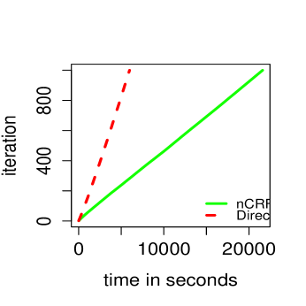
(a) Single level nHDP (HDP) : We see that direct sampling is faster than the nCRF scheme. However the difference is not as pronounced in the case with more levels

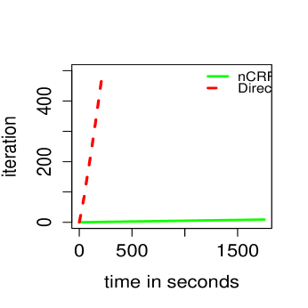
(b) two-level nHDP for ungrouped data : We see that direct sampling runs for several iterations before the nCRF technique completes the first few Gibbs sampling iterations

Figure 2: Comparison of Runtime : Direct Sampling vs nCRF

Model	Direct Sampling	nCRF
Perplexity	2230	1937

Table 2: Perplexity comparison for single level nHDP for NIPS dataset with different inference schemes

7 Non-Parametric entity-topic Modeling : Experimental Analysis

In this section, we experimentally evaluate the proposed nHDP model in the context of non-parametric entity-topic modeling, with a two-level nHDP, for the task of modeling author entities who have collaboratively written research papers, and compare its performance against available baselines. Specifically, we evaluate two different aspects: (1) how well the model is able to learn from the training samples and fit held-out data in terms of perplexity, (a) first, when all the authors are observed in training and test documents, and (b) secondly, when some of the authors are unobserved in training and test documents, (c) finally, when all authors are unobserved, to understand the effect of multi-level HDP in comparison with a single level level HDP on perplexity. (2) how accurately the model discovers hidden authors, who are not mentioned at all in the corpus.

We consider the following models for the experiments: (i) The author-topic model(ATM) (Eqn. 11) where the number of topics is pre-specified, and all authors are observed for all documents. This is used as a baseline for (1a) above. (ii) The Hierarchical Dirichlet Process (HDP) (Eqn. 3) using the direct assignment inference scheme for fair comparison. We use our own implementation for this. Recall that the HDP is infers the number of topics, and does not use author information.(iii) nHDP with completely observed entities (nHDP-co), which assumes complete entity information to be available for all documents, but is learns topics in a nonparametric fashion. This can be imagined as an improvement over ATM where the number of topics does not need to be specified. (iv) nHDP with partially observed entities (nHDP-po), which makes use of available entity information, but admits the possibility of entities being hidden globally from the corpus, or locally from individual documents. (v) nHDP with no observed entities (nHDP-no), which does not make use of any entity information and assumes all entities to be globally hidden in the corpus. For task (1a) above, the applicable models are the ATM, HDP (which ignores the entity information) and nHDP-co. For task (1b) and (1c), the ATM does not work. We evaluate HDP, and nHDP-po / nHDP-no. It is important to point out that there are no available baselines in terms of entity-topic analysis for task (2) above when some or all of the authors are unobserved.

We use the following publicly available publication datasets for our experimental analysis. The NIPS dataset is a collection of papers from Neural Information Processing Systems (NIPS) conference proceedings (volume 0-12). This collection contains 1,740 documents contributed by a total of 2,037 authors, with total 2,301,375 word tokens resulting in a vocabulary of 13,649 words. A subset of the DBLP Abstracts dataset containing 12,000 documents by 15,252 authors collected from 20 conferences records on the Digital Bibliography and Library Project (DBLP). Each document is represented as a bag of words present in abstract and title of the corresponding paper, resulting in a vocabulary size of 11,771 words.

1. Generalization Ability: We now come to our first experiment, where we evaluate the ability of the models, whose parameters are learnt from a training set, to predict words in new unseen documents in a held-out test set. We evaluate performance of a model $M$ on a test collection $D$ using the standard notion of perplexity [D. Blei and Jordan. (2003)]: $exp(-\sum_{d\in D}p(w_{d})|M)$.

In experiment (1a), all authors are observed in training and test documents. To favor the ATM, which cannot handle new authors in test document, we create test-train splits ensuring that each author in the test collection occurs in at least one training document.

Model	ATM	HDP	nHDP-co
Perplexity	2783	1775	1247

Table 3: Perplexity of ATM, HDP and nHDP-co for NIPS

Perplexity results are shown in Table 3. Recall that HDP and nHDP finds the best number of topics, while for ATM we have recorded its best performance across different value of $K$. The results show that while knowledge of authors is useful, the ability of non-parametric topic models to infer the number of topics clearly leads to better generalization ability.

Next, in experiment (1b), we first create training-test distributions with reasonable author overlap by letting each author vote with probability $0.7$ whether to send a document to train or test, and majority decision is taken for each document. Next, authors are partially hidden from both the test and the train documents as following. We iterate over the global list of authors and remove this author from all training and test documents with probability $p_{g}$. We then iterate over each training and test document, and remove each remaining author of that document with probability $p_{l}$. We experiment with different values of $p_{g}$ and $p_{l}$ to simulate different extents of missing information on authors. $p_{g}=1$ and $p_{l}=1$ corresponds to (1c), the case where authors are completely unobserved. This setting enables us to compare the two-level nHDP, with completely unobserved dishes at each level, with a HDP, to understand the relative merit of multi-level modeling over a single level in terms of perplexity.

Model	HDP	nHDP-no	nHDP-po	nHDP-po	nHDP-po	nHDP-co
$p_{g}$,$p_{l}$	1,1	1,1	0.6,0.6	0.4,0.4	0.2,0.2	0,0
Perplexity NIPS	2572	1882	1434	1266	1109	987
Perplexity DBLP	1027	997	935	869	676	394

Table 4: Perplexity for HDP and nHDP with varying percentage of hidden authors

The results are shown in Table 4. We can see that more information available about the authors, the ability to fit held-out data improves. More interestingly, even when no / very little author information is available, just the assumption about the existence of a discrete set of authors, i.e introducing an additional layer of HDP, leads to better generalization ability, corroborating the need for multi-level modeling, as can be seen from the relative performance of HDP and nHDP-no.

2. Discovering Missing Authors: Beyond data fitting, the most significant ability of our model is to discover entities which are relevant for documents in the corpus, but are never mentioned. We perform a case study with the top $6$ most prolific authors in NIPS, by removing them completely from the corpus, and then checking the ability of the model to discover them in a completely unsupervised fashion. While it is possible to define as a classification problem the task of detecting of locally missing authors in individual documents when the author is observed in other documents, we reiterate that there is no existing baseline when an author is globally hidden.

We evaluate the accuracy of discovering hidden author as follows. For each hidden author $h\in\{1\ldots H\}$, we create a $m$-dimensional vector $c_{h}$, where $m$ is the corpus size, with $c_{h}[j]$ indicating his authorship in the $j^{th}$ document. We explored two possibilities for this ‘true’ indicator vector: (a) binary indicators using the gold-standard author names for documents, and (b) the number of words written by that author in the document according to nHDP with completely observed authors (nHDP-co). Similarly, we create an $m$-dimensional vector for each new author $n\in\{1\ldots N\}$ discovered by the nHDP-po, with $c_{n}[j]$ indicating his contribution (no. of authored words) in the $j^{th}$ document. We now check how well the vectors $\{c_{n}\}$ correspond to the ‘true’ vectors $\{c_{h}\}$. This is done by defining two variables $C_{n}$ and $C_{h}$, taking values $1\ldots H$ and $1\ldots N$ respectively, and defining a joint distribution over them as $P(h,n)=\frac{1}{Z}\text{sim}(c_{h},c_{n})$, where $Z$ is a normalization constant. For $\text{sim}(c_{h},c_{n})$, we use cosine similarity between normalized versions of $c_{h}$ and $c_{n}$. Mutual information $I(C_{h},C_{n})=\sum_{h,n}p(h,n)\log\frac{p(h,n)}{p(h)p(n)}$ measures the information that $C_{h}$ and $C_{y}$ share. We used its normalized variant $NMI(C_{h},C_{n})=\frac{I(C_{h},C_{n})}{|H(C_{h})+H(C_{n})|/2}$ ($H(X)$ indicating entropy of $X$) which takes values between $0$ and $1$, higher values indicating more shared information.

First, we note that the best NMI achievable for this task, by replacing the true vectors $\{c_{h}\}$ for the discovered vectors $\{c_{n}\}$, is $0.86$ for case (a) and $0.98$ for case (b) above. In comparison, using nHDP-po, we achieve NMI scores of $0.59$ for case (a) and $0.72$ for case (b). This indicates that the actual author distributions that the model discovers not only help in fitting the data, but also have reasonable correspondence with the true hidden authors. We believe that this is a promising initial step in addressing this difficult problem.

8 Conclusions

In this paper, we have proposed the the nested Hierarchical Dirichlet Process as a prior for multi-level admixture modeling. We have also addressed the problem of entity-topic analysis from document corpora, where the set of document entities are either completely or partially hidden through the two level nHDP, which consists of two levels of Hierarchical Dirichlet Processes, where one is the base distribution of the other. We explore inference algorithms for nHDP and using a direct sampling scheme for inference, we have shown that the nHDP is able to generalize better than existing models under varying available knowledge about authors in research publications, and is additionally able to discover completely hidden authors in the corpus.

9 Appendix

9.1 Two-level Inference with Ungrouped data at Outermost Level

In this section, we describe the collapsed Gibbs sampling inference for the setting with ungrouped data at the outermost level in the entity-topic application for document modeling. This is a special case of the two level nHDP model with a DP in the outer level instead of a HDP. While we use notation similar to the nHDP inference described in section 5, the observed data is indexed by a single index $i$ (the index $j$ vanishes since there is no demarcation into groups i.e documents at the outermost level). The nCRF representation for this setting involves assigning a dish(entity) $z^{1}_{i}$ with index $k^{1}_{i}$ to every customer $i$ based on $G^{1}_{B}$, the global distribution over entities based on which the customer enters an inner level restaurant $r^{0}_{i}$. At this restaurant the customer picks a table $\hat{t}=t^{0}_{i}$ which is assigned a corresponding dish $z^{0}_{i}$ with index $k^{1}_{\hat{t}}$ that corresponds to a topic. The observed data is generated based on the topic assignment thus attained.

We now describe the two inference schemes described in section 5 for the two level nHDP for entity topic modeling for this special case of ungrouped data. Note that in section 6, an experimental comparison of both these schemes is shown.

Scheme 1: Naive nCRF based Sampling for entity-topic modeling of ungrouped data:

The latent variables to be sampled include $t^{0}_{i},k^{1}_{i}$ for each observation $i=1,\ldots,M$ and $k^{0}_{rt}$ for restaurant $r=1,\ldots,K^{1}$ and table $t=1,\ldots,T^{0}_{r}$. Sampling $k^{0}_{rt}$ is similar to that in the full nCRF inference procedure described in the previous section and is not described here.

The update for selecting the level 0 table $t^{0}_{i}$ for each customer can be obtained as follows by integrating out the appropriate $G^{0}_{r}$.

$$p(t^{0}_{i}=\hat{t},z^{1}_{i}=r|t^{0}_{-i},X,k)\propto\begin{cases}\frac{n^{0}_{r\hat{t}}}{n^{0}_{r.}+\alpha^{0}}p(x_{i}|t^{0}_{i}=\hat{t})\hfill\text{Existing $\hat{t}=1,\ldots,T^{0}_{r}$}\\ \frac{\alpha^{0}}{n^{0}_{r.}+\alpha^{0}}p(x_{i}|t^{0}_{i}=T^{0}_{r}+1)\hfill\text{New table $\hat{t}=T^{0}_{r}$}\\ \end{cases}$$ (32)

Where $p(x_{i}|t^{0}_{i}=T^{0}_{r}+1)$ can be evaluated as follows considering the different level 0 dishes that can be assigned to the new level 0 table.

$$p(x_{i}|t^{0}_{i}=T^{0}_{z^{1}_{i}}+1)=\sum_{r=1}^{K^{0}}\frac{m^{0}_{r}}{m^{0}_{.}+\gamma^{0}}p(x_{i}|z^{0}_{i}=r)+\frac{\gamma^{0}}{m^{0}_{.}+\gamma^{0}}p(x_{i}|z^{0}_{i}=K^{0}+1)$$

The overall cost of this update step is O($M$ $T^{0}_{max}$ $K^{0}$).

The update for $k^{1}_{i}$ can be obtained by integrating out $G^{1}_{B}$ as follows.

$$p(k^{1}_{i}=r|k^{1}_{-i},X,t^{0}_{-i})\propto\begin{cases}\frac{m^{1}_{r}}{m^{1}_{.}+\gamma^{1}}p(x_{i}|k^{1}_{i}=r)\hfill\text{Existing $r=1,\ldots,K^{1}$}\\ \frac{\gamma^{1}}{m^{1}_{.}+\gamma^{1}}p(x_{i}|k^{1}_{i}=K^{1}+1)\hfill\text{New table $r=K^{1}+1$}\\ \end{cases}$$ (33)

Changing the value of $k^{1}_{i}$, invalidates the existing assignment to $t^{0}_{i}$, Hence evaluating $p(x_{i}|k^{1}_{i}=r)$ requires summing over possible values of $t^{0}_{i}$ as follows

$$p(x_{i}|k^{1}_{i}=r)=\sum_{\hat{t}=1}^{T^{0}_{r}}\frac{n^{0}_{r\hat{t}}}{n^{0}_{r\hat{t}}+\alpha^{0}}p(x_{i}|t^{0}_{i}=\hat{t},k^{1}_{i}=r)+\frac{\alpha^{0}}{n^{0}_{r\hat{t}}+\alpha^{0}}p(x_{i}|t^{0}_{i}=T^{0}_{r},k^{1}_{i}=r)$$

In turn, $p(x_{i}|t^{0}_{i}=T^{0}_{r},k^{1}_{i}=r)$, corresponds to the case where a new level 0 table is created and requires summing over all potential value of level 1 dish assignments for this table. Hence, $p(x_{i}|t^{0}_{i}=T^{0}_{r},k^{1}_{i}=r$ and similarly $p(x_{i}|k^{1}_{i}=K^{1}+1)$ that involve the creation of a new level 1 table, can be evaluated as follows,

$$p(x_{i}|t^{0}_{i}=T^{0}_{r},k^{1}_{i}=r)=\sum_{r=1}^{K^{0}}\frac{m^{0}_{r}}{m^{0}_{.}+\gamma^{0}}p(x_{i}|z^{0}_{i}=r)+\frac{\gamma^{0}}{m^{0}_{.}+\gamma^{0}}p(x_{i}|z^{0}_{i}=K^{0}+1)$$

Scheme 2: Direct Sampling for entity-topic modeling of Ungrouped data
The latent variables involved in the direct sampling scheme are $z^{0}_{i}$ and $z^{1}_{i}$ for each observation $i=1,\ldots,M$. Sampling $z^{0}_{i}$ is similar to that for the case of full nHDP direct sampling

$$\begin{split}p(z^{0}_{i}=p|z^{1}_{i}=r,{\bf z^{0}_{-i}},{\bf m},\beta,{\bf x})\propto p(z^{0}_{i}=p|{\bf z^{0}_{-i}},z^{1}_{i}=r)p(x_{i}|z^{0}_{ji}=p,{\bf x_{-i}})\end{split}$$

The first term can be expanded to the following, similar to that in the full nHDP with $n^{0}_{r.p}$ defined in section 5.2.

$$p(z^{0}_{i}=p|z^{1}_{i}=r,{\bf z^{0}_{-i}})\propto\begin{cases}\frac{n^{0}_{r.p}+\alpha\beta^{0}_{p}}{n_{r,.}+\alpha^{0}}\hfill\text{ Existing dish}\\ \frac{\alpha^{0}\beta^{0}_{new}}{n^{0}_{r.}+\alpha^{0}}\hfill\text{ New dish}\end{cases}$$ (34)

The second term can be simplified similar to section 5.2 by integrating out the $\phi$ multinomials corresponding to the dishes in the inner most level.

The update for $z^{1}_{i}$ can be similarly obtained as

$$\begin{split}p(z^{1}_{i}=p|z^{1}_{-i},z^{0}_{i}=q,{\bf z^{1}_{-i}},{\bf m},\beta,{\bf x})\\ \propto p(z^{1}_{i}=p|{\bf z^{l}_{-i}})p(z^{0}_{i}=q|{\bf z^{0}_{-i}},z^{1}_{i}=p)\end{split}$$

The first term is the conditional of a simple CRP while the second term simplifies as

$$p(z^{0}_{i}=q|{\bf z^{0}_{-i}},z^{1}_{i}=p)\propto\begin{cases}\frac{n^{0}_{pq}+\alpha^{0}\beta^{0}_{q}}{n^{0}_{p.}+\alpha^{0}}\hfill\text{Existing dish}\\ \frac{\alpha^{0}\beta^{0}_{new}}{n^{0}_{p.}+\alpha^{0}}\hfill\text{New dish}\\ \end{cases}$$

References

- A. McCallum and Wang. (2004) A. Corrada-Emmanuel A. McCallum and X. Wang. The author recepient topic model for topic and role discovery in social networks. 2004.
- A. Rodriguez and Gelfand. (2008) D. Dunson A. Rodriguez and A. Gelfand. The nested dirichlet process. Journal of the American Statistical Association, 103(483):1131–1154, 2008.
- Antoniak. (1974) C. Antoniak. Mixtures of Dirichlet Processes with applications to Bayesian nonparametric problems. Ann. Statist., 2(6):1152–1174, 1974.
- Blunsom et al. (2009) Phil Blunsom, Trevor Cohn, Sharon Goldwater, and Mark Johnson. A note on the implementation of hierarchical dirichlet processes. ACL, 2009.
- D. Blei and Jordan. (2003) A. Ng D. Blei and M. Jordan. Latent dirichlet allocation. JMLR, 2003.
- D. Blei and Tanenbaum. (2010) M. Jordan D. Blei, T. Griffiths and J. Tanenbaum. The nested chinese restaurant process and bayesian nonparametric inference of topic hierarchies. JACM, 2010.
- D. Newman and Smyth. (2006) C. Chemudugunta D. Newman and P. Smyth. Statistical entity-topic models. ACM SIGKDD, pages 680–686, 2006.
- D. Wulsin and Litt. (2012) S. Jensen D. Wulsin and B. Litt. A Bayesian analysis of some nonparametric problemsa hierarchical dirichlet process model with multiple levels of clustering for human eeg seizure modeling. ICML, 2012.
- Dai and Storkey. (2009) A. Dai and A. Storkey. Author disambiguation: A nonparametric topic and co-authorship model. NIPS Workshop on Applications for Topic Models Text and Beyond, 2009.
- E. Erosheva and Lafferty. (2004) S. Fienberg E. Erosheva and J. Lafferty. Mixed-membership models of scientific publications. PANS, 101-suppl(1), 2004.
- E. Fox and Willsky. (2011) M. Jordan E. Fox, E. Sudderth and A. Willsky. A sticky hdp-hmm with application to speaker diarization. Annals of Applied Stats., 5(2A):1020–1056, 2011.
- Ferguson. (1973) T. Ferguson. A Bayesian analysis of some nonparametric problems. Ann. Statist., 1(2):209–230, 1973.
- H. Kim and Han. (2012) J. Hockenmaier H. Kim, Y. Sun and J. Han. Entity topic models for mining documents associated with entities. ICDM, pages 349–358, 2012.
- J. Paisley and Jordan. (2012) D. Blei J. Paisley, C. Wang and M. Jordan. Nested hierarchical dirichlet processes. Arxiv, 2012.
- M. Rosen-Zvi and Smyth. (2004) M. Steyvers M. Rosen-Zvi, T. Griffiths and P. Smyth. The author-topic model for authors and documents. UAI, 2004.
- Pitman. (2002) J. Pitman. Gibbs sampling methods for stick-breaking priors. Lecture Notes for St. Flour Summer School, 2002.
- Sethuraman. (1994) J. Sethuraman. A constructive definition of Dirichlet Priors. Statistica Sinica, 4:639–650, 1994.
- Sharif-razavian and Zollmann. (2008) N. Sharif-razavian and A. Zollmann. An overview of nonparametric bayesian models and applications to natural language processing. Science, pages 71–93, 2008.
- Y. Teh and Blei. (2006) M. Beal Y. Teh, M. Jordan and D. Blei. Hierarchical Dirichlet processes. Journal of the American Statistical Association, 2006.