An Efficient Implementation of Brezzi-Douglas-Marini (BDM) Mixed Finite Element Method in MATLAB

Abstract.

In this paper, a MATLAB package

dm_mfem  for a linear Brezzi-Douglas-Marini (BDM) mixed finite element
method is provided for the numerical solution of elliptic diffusion pro

lems with mixed boundary conditions on unstructured grids. BDM basis functions defined by standard barycentric coordinates are used in the paper. Local and global edge ordering are treated carefully. MATLAB build-in functions and vectorizations are used to guarantee the erectness of the programs. The package is simple and efficient, and can be easily adapted for more complicated edge-based finite element spaces. A numerical example is provided to illustrate the usage of the package.

1. Introduction

In recent years, MATLAB is widely used in the numerical simulation and is proved to be an excellent tool for academic educations. For example, Trefethen’s book on spectral methods [15] is extremely popular. In the area of finite element method, there are several papers on writing clear, short, and easily adapted MATLAB codes, for example [1, 2, 10, 11]. Vectorizations are used in [10] and [11] to guarantee the effectiveness of the MATLAB finite elements codes. The mixed finite element [13, 3, 4] is now widely used in many area of scientific computation. For example, in [5, 6, 7, 8, 9], we use RT(Rviart-Thomas)/BDM(Brezzi-Douglas-Marini) space to build recovery-based a posteriori error estimators. On the other side, except for the clear presentation of [2] on $RT_{0}$, the implementation of more complicated BDM elements is still somehow confusing for researchers and students. The purpose of this paper is to fill this gap by giving a simple, efficient, and easily adaptable MATLAB implementation of $B\!D\!M_{1}$-$P_{0}$ mixed finite element methods for of elliptic diffusion problems with mixed boundary conditions on unstructured grids.

For linear BDM elements, there are several versions to write the basis functions explicitly. In [4, 14], basis functions are defined on each elements using heights and normal vectors. This version of basis functions is less straightforward than the basis functions defined by barycentric coordinates. After all, everyone is very familiar with barycentric coordinates in finite element programmings. Thus, in this implementation, we will use the definition which only uses barycentric coordinates.

There are two basis functions on each edge for linear BDM elements. Unlike the RT element, BDM basis functions depend on the stating and terminal points of the edge. Thus, when assembling the local matrix, for a local edge on each element, we need to make sure we find its correct global stating and terminal points of the edge. There is an implementation of BDM element in $i$FEM package [10] https://bitbucket.org/ifem/ifem/. But in order to make the local ordering of edges in an element is the same as the global ordering of edges, the triangles are not always counterclockwisely oriented. This will cause confusion for programmers. And if we use this ordering, sometime we may need two kinds of element map, one is counterclockwisely ordered, the other is ordered by the indices of vertices. This will make things more complicated. In this implementation, we will use the standard counterclockwisely ordering of vertices of triangles.

Besides these issues, to get the right convergence order, we need to handle the boundary conditions carefully. In this package, we use the basic data structure of $i$FEM [10], and full MATLAB vectorization is used.

In a summery, in this package:

1. $B\!D\!M_{1}$ basis functions are explicitly defined using barycentric coordinates.

2. Elements are still positively oriented. A function is used to find the right global stating and terminal vertices of an edge in a local element.

3. Mixed type of boundary conditions are handled correctly to guarantee the right order of convergence.

4. MATLAB build-in functions and vectorizations are used to guarantee the erectness of the programs.

The package can be download from http://personal.cityu.edu.hk/~szhang26/bdm_mfem.zip.

The paper is organized as follows. Section 2 describes the model diffusion problem, its $B\!D\!M_{1}$-$P_{0}$ mixed finite element approximation and the corresponding matrix problem. Section 3 introduces a simple example problem to demonstrate out MATLAB code. In Section 4, edge-based linear BDM basis functions are defined. The main part of the code for the matrix problem is discussed in Section 6. MATLAB functions to checking the errors are discussed in Section 7. Finally, we discuss some related finite elements in Section 8.

2. Model problem and BDM1-P0 mixed finite element method

2.1. Model problem

Let $\Omega$ be a bounded polygonal domain in $\Re^{2}$, with boundary $\partial\Omega=\bar{\Gamma}_{{}_{D}}\cup\bar{\Gamma}_{{}_{N}}$, $\Gamma_{{}_{D}}\cap\Gamma_{{}_{N}}=\emptyset$, and $\mbox{measure}\,(\Gamma_{D})\not=0$, and let ${\bf n}$ be the outward unit vector normal to the boundary. For a vector function $\mbox{\boldmath$\tau$}=(\mbox{\boldmath$\tau$}_{1},\mbox{\boldmath$\tau$}_{2})$, define the divergence and curl operators by $\nabla\cdot\mbox{\boldmath$\tau$}=\frac{\partial\mbox{\boldmath$\tau$}_{1}}{\partial x_{1}}+\frac{\partial\mbox{\boldmath$\tau$}_{2}}{\partial x_{2}}$ and $\nabla\times\mbox{\boldmath$\tau$}=\frac{\partial\mbox{\boldmath$\tau$}_{2}}{\partial x_{1}}-\frac{\partial\mbox{\boldmath$\tau$}_{1}}{\partial x_{2}}$. For a function $v$, define the gradient and rotation operators by $\nabla v=(\frac{\partial v}{\partial x_{1}},\frac{\partial v}{\partial x_{2}})^{t}$ and $\nabla^{\perp}v=(\frac{\partial v}{\partial x_{2}},-\frac{\partial v}{\partial x_{1}})^{t}$.

Consider diffusion equation

(2.1) $$-\nabla\cdot(\alpha(x)\nabla u)=f\quad\mbox{in}\quad\Omega\\$$

with boundary conditions

(2.2) $$-\alpha\nabla u\cdot{\bf n}=g_{N}\quad\mbox{on}\quad\Gamma_{N}\quad\mbox{and}\quad u=g_{D}\quad\mbox{on}\quad\Gamma_{D}.$$

We assume that the right-hand side $f\in L^{2}(\Omega)$, $g_{D}$ in $H^{1/2}(\Gamma_{D})$, and that $g_{N}\in L^{2}(\Gamma_{N})$, and that $\alpha(x)$ is a positive piecewise constant function. Define the flux by $\mbox{\boldmath$\sigma$}=-\alpha(x)\nabla u$, then we have

(2.3) $$\alpha^{-1}\mbox{\boldmath$\sigma$}=-\nabla u\quad\mbox{and}\quad\nabla\cdot\mbox{\boldmath$\sigma$}=f.$$

Define the standard $H({\rm div};\,\Omega)$ spaces as

$$H({\rm div};\,\Omega) := \{\mbox{\boldmath$\tau$}\in L^{2}(\Omega)^{2}:\nabla\cdot\mbox{\boldmath$\tau$}\in L^{2}(\Omega)\},$$

$$H_{N}({\rm div};\Omega) := \{\mbox{\boldmath$\tau$}\in H({\rm div};\,\Omega):\mbox{\boldmath$\tau$}\cdot{\bf n}=0\mbox{ on }\Gamma_{N}\}.$$

Multiply the first equation in (2.3) by a $\mbox{\boldmath$\tau$}\in H_{N}({\rm div};\Omega)$ and integrating by parts, we get

$$(\alpha^{-1}\mbox{\boldmath$\sigma$},\mbox{\boldmath$\tau$})=-(\nabla u,\mbox{\boldmath$\tau$})=(\nabla\cdot\mbox{\boldmath$\tau$},v)-(\mbox{\boldmath$\tau$}\cdot{\bf n},g_{D})_{\Gamma_{D}}$$

where $(\cdot,\cdot)_{\omega}$ is the $L^{2}$ inner product on a domain $\omega$. If $\omega=\Omega$, we omit the subscript. Then the mixed variational formulation is to find $(\mbox{\boldmath$\sigma$},\,u)\in H({\rm div};\Omega)\times L^{2}(\Omega)$ with $\mbox{\boldmath$\sigma$}\cdot{\bf n}=g_{N}$ on $\Gamma_{N}$, such that

(2.4) $$\left\{\begin{array}[]{lclll}(\alpha^{-1}\mbox{\boldmath$\sigma$},\,\mbox{\boldmath$\tau$})-(\nabla\cdot\mbox{\boldmath$\tau$},\,u)&=&-(\mbox{\boldmath$\tau$}\cdot{\bf n},g_{D})_{\Gamma_{D}}&\forall\,\,\mbox{\boldmath$\tau$}\in H_{N}({\rm div};\Omega),\\[5.69054pt] (\nabla\cdot\mbox{\boldmath$\sigma$},\,v)&=&(f,\,v)&\forall\,\,v\in L^{2}(\Omega).\end{array}\right.$$

The existence, uniqueness, and stability results of (2.4) are well-known, and can be found in standard references, for example, [4].

2.2. $B\!D\!M_{1}$-$P_{0}$ mixed formulation

Let ${\mathcal{T}}=\{K\}$ be a regular triangulation of the domain $\Omega$. Denote the set of all edges of the triangulation by ${\mathcal{E}}:={\mathcal{E}}_{I}\cup{\mathcal{E}}_{D}\cup{\mathcal{E}}_{N},$ where ${\mathcal{E}}_{I}$ is the set of all interior element edges and ${\mathcal{E}}_{D}$ and ${\mathcal{E}}_{N}$ are the sets of all boundary edges belonging to the respective $\Gamma_{D}$ and $\Gamma_{N}$. For any element $K\in{\mathcal{T}}$, denote by $P_{k}(K)$ the space of polynomials on $K$ with total degree less than or equal to $k$. The $H({\rm div};\,\Omega)$ conforming Brezzi-Douglas-Marini (BDM) space [3] of the lowest order is defined by

$$B\!D\!M_{1}=\{\mbox{\boldmath$\tau$}:\mbox{\boldmath$\tau$}|_{K}\in B\!D\!M_{1}(K),\forall K\in{\mathcal{T}}\}\quad\mbox{with}\quad B\!D\!M_{1}(K)=P_{1}(K)^{2}.$$

and let $B\!D\!M_{1,N}=B\!D\!M_{1}\cap H_{N}({\rm div};\Omega)$. The piecewise constant space $P_{0}$ is defined by

$$P_{0}=\{v:v|_{K}\in P_{0}(K),\;\forall K\in{\mathcal{T}}\}.$$

For simplicity, we further assume that $\alpha$ is a positive constant in each element $K\in{\mathcal{T}}$. Let ${\mathcal{T}}_{N}$ be the one dimensional mesh induced by ${\mathcal{T}}$ on $\Gamma_{N}$. Define

$$P_{1}({\mathcal{T}}_{N})=\{v:v|_{E}\in P_{1}(E),\;\;\forall E\in{\mathcal{T}}_{N}\}.$$

Let $g_{N,h}$ be the $L^{2}$ projection of $g_{N}$ on $P_{1}({\mathcal{T}}_{N})$. The $B\!D\!M_{1}$-$P_{0}$ mixed finite element discrete problem then is to find $(\mbox{\boldmath$\sigma$}_{h},u_{h})\in BDM_{1}\times P_{0}$ with $\mbox{\boldmath$\sigma$}_{h}\cdot{\bf n}=g_{N,h}$ on $\Gamma_{N}$, such that

(2.5) $$\left\{\begin{array}[]{lclll}(\alpha^{-1}\mbox{\boldmath$\sigma$}_{h},\,\mbox{\boldmath$\tau$}_{h})-(\nabla\cdot\mbox{\boldmath$\tau$}_{h},\,u_{h})&=&-(\mbox{\boldmath$\tau$}_{h}\cdot{\bf n},g_{D})_{\Gamma_{D}}&\forall\,\,\mbox{\boldmath$\tau$}_{h}\in B\!D\!M_{1,N},\\[5.69054pt] -(\nabla\cdot\mbox{\boldmath$\sigma$}_{h},\,v_{h})&=&-(f,\,v_{h})&\forall\,\,v_{h}\in P_{0}.\end{array}\right.$$

The discrete problem (2.5) has a unique solution, and the following error estimates hold assuming that the solution $(\mbox{\boldmath$\sigma$},u)$ has enough regularity:

(2.6) $$\|\alpha^{-1/2}(\mbox{\boldmath$\sigma$}-\mbox{\boldmath$\sigma$}_{h})\|_{0}\leq Ch^{2}\|\alpha^{-1/2}\mbox{\boldmath$\sigma$}\|_{2}\quad\mbox{and}\quad\|u-u_{h}\|_{0}\leq C(h\|u\|_{1}+h^{2}\|\mbox{\boldmath$\sigma$}\|_{2}),$$

where $h$ is the mesh size and $\|\cdot\|_{k}$ is the standard norm of Sobolev space $H^{k}$. Thus, we should expect order 2 convergence of $\sigma$ and order 1 convergence of $u$ if the solution is smooth enough.

Let $\mbox{\boldmath$\sigma$}_{N}\in B\!D\!M_{1}$ be the interpolation of $g_{N,h}$ on $\Gamma_{N}$ (The construction of $\mbox{\boldmath$\sigma$}_{N}$ will be explained in Section LABEL:BCrhside in detail). Then $\mbox{\boldmath$\sigma$}_{h}=\mbox{\boldmath$\sigma$}_{N}+\mbox{\boldmath$\sigma$}_{0}$, with $\mbox{\boldmath$\sigma$}_{0}\in B\!D\!M_{1,N}$ solves the following discrete problem:

(2.7) $$\left\{\begin{array}[]{llll}(\alpha^{-1}\mbox{\boldmath$\sigma$}_{0},\mbox{\boldmath$\tau$}_{h})-(\nabla\cdot\mbox{\boldmath$\tau$}_{h},\,u_{h})&=&-(\mbox{\boldmath$\tau$}_{h}\cdot{\bf n},g_{D})_{\Gamma_{D}}-(\alpha^{-1}\mbox{\boldmath$\sigma$}_{N},\mbox{\boldmath$\tau$}_{h})&\forall\;\mbox{\boldmath$\tau$}_{h}\in B\!D\!M_{1,N},\\[5.69054pt] -(\nabla\cdot\mbox{\boldmath$\sigma$}_{0},\,v_{h})&=&-(f,\,v_{h})+(\nabla\cdot\mbox{\boldmath$\sigma$}_{N},\,v_{h})&\forall\,\,v_{h}\in P_{0}.\end{array}\right.$$

2.3. Matrix problem

Suppose that all edges are uniquely defined with fixed initial and terminal vertices, in Section 5, we will define two basis functions $\mbox{\boldmath$\phi$}_{j,1}$ and $\mbox{\boldmath$\phi$}_{j,2}$ for an edge $E_{j}\in{\mathcal{E}}$, $j=1,\cdots,N\!E$, with $N\!E$ is the number of edges. For simplicity, we assume that the total number of all edges in ${\mathcal{E}}_{I}$ and ${\mathcal{E}}_{D}$ is $M$, and $B\!D\!M_{1,N}=\mbox{span}\{\mbox{\boldmath$\phi$}_{j,1},\mbox{\boldmath$\phi$}_{j,2},j=1\cdots,M\}$ (The real mesh may has a different order of indices). The basis of $P_{0}$ is very simple. For the element $K_{j}$, its basis is $1_{j}$ which is $1$ on $K_{j}$ and $0$ elsewhere.

We want to compute the coefficient vectors ${\bf x}\in\rm I\kern-1.90002ptR^{2NE}$ of $\mbox{\boldmath$\sigma$}_{h}$ and ${\bf y}\in\rm I\kern-1.90002ptR^{NT}$ of $u_{h}$ with respect to the $B\!D\!M_{1}$ basis and $P_{0}$ basis

(2.8) $$\mbox{\boldmath$\sigma$}_{h}=\sum_{j=1}^{N\!E}\left(x_{j}\phi_{j,1}+x_{N\!E+j}\phi_{j,2}\right)\quad\mbox{and}\quad u_{h}=\sum_{k=1}^{NT}y_{k}1_{k},$$

and

(2.9) $$\mbox{\boldmath$\sigma$}_{N}=\sum_{j=M+1}^{N\!E}(x_{j}\phi_{j,1}+x_{N\!E+j}\phi_{j,2})$$

with $x_{j}$ and $x_{N\!E+j}$ are determined by $g_{N,h}$ (discussed later in Section LABEL:BCrhside). Then

$$\sum_{j=1}^{M}\left(x_{j}(\alpha^{-1}\mbox{\boldmath$\phi$}_{i,1},\mbox{\boldmath$\phi$}_{j,1})+x_{j+N\!E}(\alpha^{-1}\mbox{\boldmath$\phi$}_{i,1},\mbox{\boldmath$\phi$}_{j,2})\right)-\sum_{k=1}^{NT}y_{k}(\mbox{\boldmath$\phi$}_{i,1},1)_{K_{k}}$$

$$\quad=-(g_{D},\mbox{\boldmath$\phi$}_{i,1}\cdot{\bf n}_{\Omega})_{\Gamma_{D}}-\sum_{j=M+1}^{N\!E}(x_{j}(\alpha^{-1}\mbox{\boldmath$\phi$}_{i,1},\mbox{\boldmath$\phi$}_{j,1})+x_{j+N\!E}(\alpha^{-1}\mbox{\boldmath$\phi$}_{i,1},\mbox{\boldmath$\phi$}_{j,2}));$$

$$\sum_{j=1}^{M}\left(x_{j}(\alpha^{-1}\mbox{\boldmath$\phi$}_{i,2},\mbox{\boldmath$\phi$}_{j,1})+x_{j+N\!E}(\alpha^{-1}\mbox{\boldmath$\phi$}_{i,2},\mbox{\boldmath$\phi$}_{j,2})\right)-\sum_{k=1}^{NT}y_{k}(\mbox{\boldmath$\phi$}_{i,2},1)_{K_{k}}$$

$$\quad=-(g_{D},\mbox{\boldmath$\phi$}_{i,2}\cdot{\bf n}_{\Omega})_{\Gamma_{D}}-\sum_{j=M+1}^{N\!E}(x_{j}(\alpha^{-1}\mbox{\boldmath$\phi$}_{i,2},\mbox{\boldmath$\phi$}_{j,1})+x_{j+N\!E}(\alpha^{-1}\mbox{\boldmath$\phi$}_{i,2},\mbox{\boldmath$\phi$}_{j,2}));$$

$$-\sum_{j=1}^{M}\left(x_{j}(\mbox{\boldmath$\phi$}_{j,1},1)_{K_{\ell}}+x_{j+N\!E}(\mbox{\boldmath$\phi$}_{j,2},1)_{K_{\ell}}\right)$$

$$\quad=-(f,1)_{K_{\ell}}+\sum_{j=M+1}^{N\!E}\left(x_{j}(\nabla\cdot\mbox{\boldmath$\phi$}_{j,1},1)_{K_{\ell}}+x_{j+N\!E}(\nabla\cdot\mbox{\boldmath$\phi$}_{j,2},1)_{K_{\ell}}\right);$$

for $i=1,\cdots,M$, $\ell=1,\cdots,NT$. The coefficients $x_{j}$, $x_{j+N\!E}$, $j=M+1,\cdots,N\!E$ are known from $g_{N,h}$. Rewrite it as a matrix problem, we have

(2.10) $$\left(\begin{array}[]{ccc}B&C^{t}\\ C&0\end{array}\right)\left(\begin{array}[]{ccc}{\bf x}\\ {\bf y}\end{array}\right)=\left(\begin{array}[]{ccc}b1\\ b2\end{array}\right),$$

where $B$ is a $2M\times 2M$ matrix and $C$ is a $NT\times 2M$ matrix with entries:

(2.11) $$\begin{array}[]{lllllllll}B_{i,j}=(\alpha^{-1}\mbox{\boldmath$\phi$}_{i,1},\mbox{\boldmath$\phi$}_{j,1}),&B_{i,j+M}=(\alpha^{-1}\mbox{\boldmath$\phi$}_{i,1},\mbox{\boldmath$\phi$}_{j,2}),&B_{i+M,j}=(\alpha^{-1}\mbox{\boldmath$\phi$}_{i,2},\mbox{\boldmath$\phi$}_{j,1}),\\ B_{i+M,j+M}=(\alpha^{-1}\mbox{\boldmath$\phi$}_{i,2},\mbox{\boldmath$\phi$}_{j,2}),&C_{\ell,j}=-(\nabla\cdot\mbox{\boldmath$\phi$}_{j,1},1_{\ell}),&C_{\ell,j+M}=-(\nabla\cdot\mbox{\boldmath$\phi$}_{ij2},1_{\ell}),\end{array}$$

where $i=1,\cdots,M$, $j=1,\cdots,M$, and $\ell=1,\cdots,NT$; and the right hand side where $b1$ is a $2M\times 1$ vectors and $b2$ is an $NT\times 1$ vector with entries

$$b1_{i} = -(g_{D},\mbox{\boldmath$\phi$}_{i,1}\cdot{\bf n}_{\Omega})_{\Gamma_{D}}-\sum_{j=M+1}^{N\!E}(x_{j}(\alpha^{-1}\mbox{\boldmath$\phi$}_{i,1},\mbox{\boldmath$\phi$}_{j,1})+x_{j+N\!E}(\alpha^{-1}\mbox{\boldmath$\phi$}_{i,1},\mbox{\boldmath$\phi$}_{j,2}));$$

$$b1_{i+M} = -(g_{D},\mbox{\boldmath$\phi$}_{i,2}\cdot{\bf n}_{\Omega})_{\Gamma_{D}}-\sum_{j=M+1}^{N\!E}(x_{j}(\alpha^{-1}\mbox{\boldmath$\phi$}_{i,2},\mbox{\boldmath$\phi$}_{j,1})+x_{j+N\!E}(\alpha^{-1}\mbox{\boldmath$\phi$}_{i,2},\mbox{\boldmath$\phi$}_{j,2}));$$

$$b2_{\ell} = -(f,1)_{K_{\ell}}+\sum_{j=M+1}^{NE}(x_{j}(\nabla\cdot\mbox{\boldmath$\phi$}_{j,1},1)_{K_{\ell}}+x_{j+N\!E}(\nabla\cdot\mbox{\boldmath$\phi$}_{j,2},1)_{K_{\ell}})$$

where $i=1,\cdots,M$ and $\ell=1,\cdots,NT$; $(x_{1},\cdots,x_{M},x_{1+NE},\cdots,x_{M+NE},y_{1},\cdots,y_{NT})^{t}$ is the $2M+NT\times 1$ solution vector.

3. A Numerical Example

We will demonstrate our MATLAB program by a simple test problem. Let $\Omega=(-1,1)^{2}$, with $\Gamma_{N}=\{x\in(-1,1)\}\times\{y=1\}$, and the rest is $\Gamma_{D}$ The mesh is given in Fig. 2. We choose the diffusion coefficient and the exact solution to be

$$\alpha=\left\{\begin{array}[]{lll}10&\mbox{if }x<0;\\ 1&\mbox{if }x>0;\end{array}\right.\quad\mbox{and}\quad u(x,y)=\left\{\begin{array}[]{lll}(x^{2}y^{2}+x)/10+y&\mbox{if }x<0;\\ x^{2}y^{2}+x+y&\mbox{if }x>0.\end{array}\right.$$

The right-hand side $f=-2(x^{2}+y^{2})$. The exact $\sigma$ is

$$\mbox{\boldmath$\sigma$}(x,y)=\left\{\begin{array}[]{lll}-(2xy^{2}+1,2x^{2}y+10)^{t}&\mbox{if }x<0;\\ -(2xy^{2}+1,2x^{2}y+1)^{t}&\mbox{if }x>0.\end{array}\right.$$

It’s clear that $\sigma$ itself is not continuous, but its normal component is continuous. The boundary conditions are

$$u(x,y)=\left\{\begin{array}[]{lll}y^{2}/10+y-1/10&\mbox{if }x=-1;\\ y^{2}+y+1&\mbox{if }x=1;\\ (x^{2}+x)/10-1&\mbox{if }x<0\mbox{ and }y=-1;\\ x^{2}+x-1&\mbox{if }x>0\mbox{ and }y=-1;\end{array}\right.$$

and

$$-\alpha\nabla u\cdot(0,1)^{t}=g_{N}=\left\{\begin{array}[]{lll}-2x^{2}-10&\mbox{if }x<0\mbox{ and }y=1;\\ -2x^{2}-1&\mbox{if }x>0\mbox{ and }y=1.\end{array}\right.$$

We choose this exact solution to emphasize that the flux $\sigma$ is in $H({\rm div};\Omega)$, but not the $\nabla u$. The main MATLAB codes of $\alpha$, $f$, $g_{D}$ and $g_{N}$ are given in ctalpha.m, , m, and m respectively. Here the Dirichlet boundary condition is given by the exact solution in m for simplicity.

Listing 1: exactalpha, f, gD, and gN

⬇

1ction z = exactalpha(p)

2ix = (p(:,1)<0); z = ones(size(p,1),1); z(ix) = 10.0;

3end

4function z = f(p)

5x = p(:,1); y = p(:,2); z = -2*(x.*x+y.*y);

6end

7function z = gD(p)

8x = p(:,1); y = p(:,2);

9z=(x<0).*(0.1*x.*x.*y.*y+0.1*x+y)+(x>=0).*(x.*x.*y.*y+x+y);

10end

11function z = gN(p)

12x = p(:,1); y = p(:,2); z=(x<0).*(-2*x.*x-10)+(x>=0).*(-2*x.*x-1);

13end

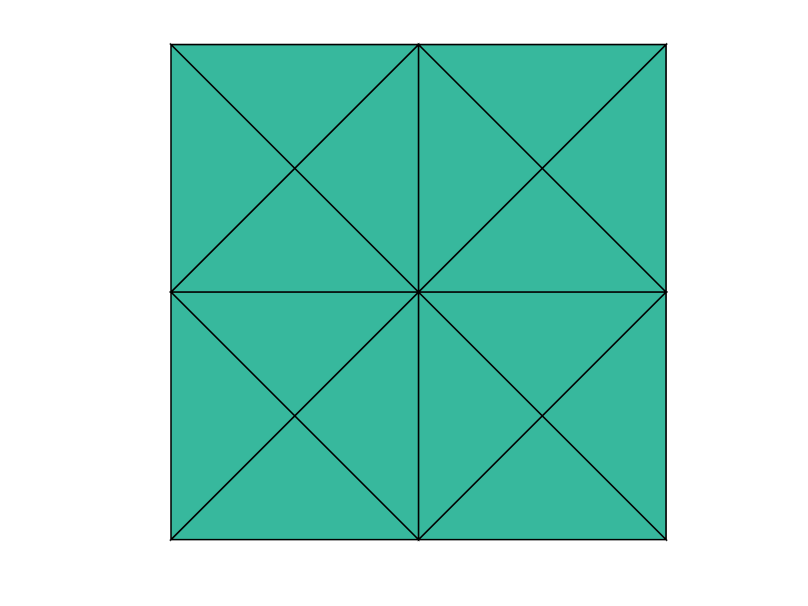
Figure 1. mesh of the example

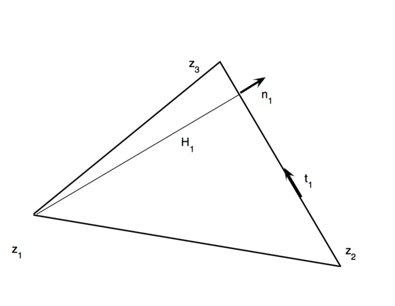
Figure 2. a triangle

The MATLAB program to solve this problem is given in n.m. Lines 2-7 read the essential geometric data of the problem. Line 9 generates the edges, and other necessary geometric relations. Lines 11-12 solve the problem by the $B\!D\!M_{1}$ mixed finite element method.

Listing 2: main.m

⬇

1%% Geometry settingde = [-1 1; 0 1; 1 1; -0.5 0.5; 0.5 0.5; -1 0; 0 0; 1 0; ...

2 -0.5 -0.5; 0.5 -0.5;-1.0 -1.0; 0.0 -1.0;1.0 -1.0];

3elem =[4 2 1;4 1 6;4 6 7;4 7 2;5 3 2;5 2 7;5 7 8;5 8 3;9 7 6;...

4 9 6 11;9 11 12;9 12 7;10 8 7;10 7 12;10 12 13;10 13 8];

5bdEdge = [2 0 0;1 0 0; 0 0 0;0 0 0;2 0 0;0 0 0;0 0 0;1 0 0;...

6 0 0 0;1 0 0;1 0 0;0 0 0;0 0 0;0 0 0;1 0 0;1 0 0];

7%% Geometric relations

8[edge,elem2edge,signedge] = geomrelations(elem);

9%%

10[sigma,u] = diffusionbdm(node,elem,bdEdge,elem2edge,edge,...

11 signedge,@exactalpha,@f,@gD,@gN);

4. Triangulation and geometric data structures

4.1. Geometric description and geometric relations

We follow [10] for the data representation of the set of all vertices, the regular triangulation ${\mathcal{T}}$, the edges, and the boundaries.

The set of all vertices ${\mathcal{N}}=\{z_{1},\cdots,z_{N}\}$ is represented by an N$\times 2$ matrix e(1:N,1:2), where $N$ is the number of vertices, and the $i$-th row of e is the coordinates of the $i$-th vertex $z_{i}=(x_{i},y_{i})$, e(i,:) = [xi,yi]. Lines 2-3 of n.m give the e of our example. For example, the 1st vertex has coordinates $x_{1}=-1$ and $y_{1}=1$.

The triangulation ${\mathcal{T}}$ is represented by an NT$\times 3$ matrix m(1:NT,1:3) with NT the number of elements. The $i$-th element $K_{i}=\mbox{conv}\{z_{i},z_{j},z_{k}\}$ is stored as m(i,:) = [i j k], where the vertices are given in the counterclockwise order. Lines 4-5 of n.m give the m of our example. For example, the 1st element $K_{1}$ has three vertices in the order of $z_{4}$, $z_{2}$ and $z_{1}$.

We call the the opposite edge of the $i$-th vertex, $i=1,2,3$ of a triangle the $i$-th edge of the triangle.

The matrix dge(1:NT, 1:3) indicates which edge of an element is on the boundary of the domain. For a non-boundary edge, the value is $0$; the value is $1$ or $2$ for a Dirichlet or Neumann boundary edge respectively. Lines 4-5 of n.m give the dge of our example. For example, the 1st element $K_{1}$ has three edge, the first edge is on the Neumann boundary, and the other two are not on the boundary.

Listing 3: geomrelations.m

⬇

1ction [edge,elem2edge,signedge] = geomrelations(elem)

2NT = size(elem,1);

3totalEdge = sort([elem(:,[2,3]); elem(:,[3,1]); elem(:,[1,2])],2);

4[edge, useless, j] = unique(totalEdge, 'rows');

5elem2edge = reshape(j,NT,3);

6

7signedge = ones(NT,3);

8signedge(:,1) = signedge(:,1) - 2* (elem(:,2)>elem(:,3));

9signedge(:,2) = signedge(:,2) - 2* (elem(:,3)>elem(:,1));

10signedge(:,3) = signedge(:,3) - 2* (elem(:,1)>elem(:,2));

11end

The MATLAB code mrelations.m generates e, m2edge, and nedge. The explanations of these codes can be found in [10].

The matrix e(1:NE,1:2) is defined with NE the total number of edges, and the $k$-th edge $E_{k}$ with the starting vertex $z_{i}$ and the terminal vertex $z_{j}$ is stored as e(k,:) = [i j]. We always ensure that e(k,1) < edge(k,2). Lines 3-4 of mrelations.m generate e. For our example, 28 and e=[1 2; 1 4; 1 6;2 3;2 4;2 5;2 7;3 5;3 8;4 6;4 7;5 7;5 8;6 7;6 9;6 11;7 8;7 9;7 10;7 12;8 10;8 13;9 11;9 12;10 12;10 13;11 12;12 13]. For example, the 2nd edge’s starting vertex is $z_{1}$ and terminal vertex is $z_{4}$.

For an edge $E_{j}$ with the starting vertex $z_{s}$ and the terminal vertex $z_{t}$, its normal direction is defined as $(y_{t}-y_{s},x_{s}-x_{t})^{t}/|E_{j}|$.

The matrix m2edge(1:NT,1:3) is the matrix whose $k$-th row represents the 3 global indices of the edges in the order of local edges. Line 5 of mrelations.m generates m2edge. For our example, m2edge=[1 2 5;3 10 2;14 11 10;7 5 11;4 6 8;7 12 6;17 13 12;9 8 13;14 15 18;16 23 15;27 24 23;20 18 24;17 19 21;20 25 19;28 26 25;22 21 26]. For example, the 2nd element’s three edges are $E_{3}$, $E_{10}$, and $E_{2}$.

Each edge has its fixed global orientation, while on each element, it has a local orientation, alEdge=[2 3;3 1;1 2]. The matrix nedge is an NT$\times 3$ matrix with value $1$ denoting the local and global orientations are the same, and $-1$ denoting that they are different. For our example, nedge=[-1 1 -1;1 -1 -1;1 -1 1;-1 1 1;-1 1 -1;1 -1 -1;1 -1 1;-1 1 1;-1 1 -1;1 -1 -1;1 -1 1;-1 1 1;-1 1 -1;1 -1 -1;1 -1 1;-1 1 1].

4.2. Barycentric coordinate and its gradient

On an element $K$ with counterclockwise vertices $\{z_{1},z_{2},z_{3}\}$, we define the barycentric coordinate $\lambda_{i}=(a_{i}x+b_{i}y+c_{i})/(2|K|)$, $i=1,2,3$, such that $\lambda_{i}(z_{j})=\delta_{ij}$. We only need to compute the gradient (and curl, rot, div) operators in this paper, so we only need to compute $a_{i}$, $b_{i}$, and the area $|K|$. The formulas are

$$\nabla\lambda_{i}=\displaystyle\frac{1}{2|K|}\left(\begin{array}[]{ccc}y_{i+1}-y_{i+2}\\ x_{i+2}-x_{i+1}\end{array}\right)\quad\mbox{and}\quad 2|K|=\det\left(\begin{array}[]{ccc}x_{2}-x_{1}&x_{3}-x_{1}\\ y_{2}-y_{1}&y_{3}-y_{1}\end{array}\right).$$

The function dlambda.m computes the coefficients a, b, and a. Here a and b are two NT$\times 3$ matrices, with each row stores the coefficients $a$ and $b$ for the three barycentric coordinates of corresponding 3 vertices.

Listing 4: gradlambda.m

⬇

1ction [a,b,area] = gradlambda(node,elem)

2n1 = elem(:,1); n2 = elem(:,2); n3 = elem(:,3);

3NT = size(elem,1); a = zeros(NT,3); b = zeros(NT,3);

4a(:,1) = node(n2,2)-node(n3,2); b(:,1) = node(n3,1)-node(n2,1);

5a(:,2) = node(n3,2)-node(n1,2); b(:,2) = node(n1,1)-node(n3,1);

6a(:,3) = node(n1,2)-node(n2,2); b(:,3) = node(n2,1)-node(n1,1);

7area = (a(:,2).*b(:,3)-a(:,3).*b(:,2))/2.0;

8end

4.3. Normal and tangential vectors

On a local element $K$ with counterclockwise oriented vertices $\{z_{1},z_{2},z_{3}\}$, and $E_{1}=\{z_{2},z_{3}\}$, $E_{2}=\{z_{3},z_{1}\}$, and $E_{3}=\{z_{1},z_{2}\}$ (Figure 2), we will discuss the $\nabla$ and $\nabla^{\perp}$ of $\lambda_{2}$ as examples:

$$\nabla^{\perp}\lambda_{2}=\displaystyle\frac{1}{2|K|}\left(\begin{array}[]{ccc}y_{3}-y_{1}\\ x_{1}-x_{3}\end{array}\right)\quad\mbox{and}\quad\nabla^{\perp}\lambda_{2}=\displaystyle\frac{1}{2|K|}\left(\begin{array}[]{ccc}x_{1}-x_{3}\\ y_{1}-y_{3}\end{array}\right).$$

where $|K|$ is the area of $K$. On edge $E_{1}=\{z_{2},z_{3}\}$, the unit tangential and normal vectors are

$${\bf t}_{E_{1}}=\displaystyle\frac{1}{|E_{1}|}\left(\begin{array}[]{ccc}x_{3}-x_{2}\\ y_{3}-y_{2}\end{array}\right)\quad\mbox{and}\quad{\bf n}_{E_{1}}=\displaystyle\frac{1}{|E_{1}|}\left(\begin{array}[]{ccc}y_{3}-y_{2}\\ x_{2}-x_{3}\end{array}\right).$$

where $|E|$ is the length of $E$. From Figure 2, we have $\left(\begin{array}[]{ccc}x_{1}-x_{3}\\ y_{1}-y_{3}\end{array}\right)\cdot{\bf n}_{E_{1}}=\left(\begin{array}[]{ccc}y_{3}-y_{1}\\ x_{1}-x_{3}\end{array}\right)\cdot{\bf t}_{E_{1}}=-H_{1}$, with $H_{1}$ is the height of $K_{1}$ on $E_{1}$. Now, by the fact $2|K|=|E_{1}|\cdot H_{1}$, we have

$$\nabla^{\perp}\lambda_{2}\cdot{\bf n}_{E_{1}}=\nabla\lambda_{2}\cdot{\bf t}_{E_{1}}=-1/|E_{1}|.$$

Similarly,

$$\nabla^{\perp}\lambda_{3}\cdot{\bf n}_{E_{1}}=\nabla\lambda_{3}\cdot{\bf t}_{E_{1}}=1/|E_{1}|.$$

On the hand, since the tangential and normal vectors of an edge are orthogonal, we have

(4.1) $$\nabla^{\perp}\lambda_{2}\cdot{\bf n}_{E_{2}}=\nabla^{\perp}\lambda_{3}\cdot{\bf n}_{E_{3}}=0.$$

Globally, on $E_{\ell}=\{z_{s},z_{t}\}$ ($s<t$), the unit tangential and normal vectors are

$${\bf t}_{E_{\ell}}=\displaystyle\frac{1}{|E_{\ell}|}\left(\begin{array}[]{ccc}x_{t}-x_{s}\\ y_{t}-y_{s}\end{array}\right)\quad\mbox{and}\quad{\bf n}_{E_{\ell}}=\displaystyle\frac{1}{|E_{\ell}|}\left(\begin{array}[]{ccc}y_{t}-y_{s}\\ x_{s}-x_{t}\end{array}\right).$$

We call the adjacent element whose out unit normal vector is the same as ${\bf n}_{E_{\ell}}$ as $K^{-}_{\ell}$, and the element whose out unit normal vector is the opposite of ${\bf n}_{E_{\ell}}$ as $K^{+}_{\ell}$. On both $K_{\ell}^{-}$ and $K_{\ell}^{+}$, we have

(4.2) $$\nabla^{\perp}\lambda_{s}\cdot{\bf n}_{E_{\ell}}=\nabla\lambda_{s}\cdot{\bf t}_{E_{\ell}}=-1/|E_{\ell}|\quad\mbox{and}\quad\nabla^{\perp}\lambda_{t}\cdot{\bf n}_{E_{\ell}}=\nabla\lambda_{t}\cdot{\bf t}_{E_{\ell}}=1/|E_{\ell}|.$$

5. Constructions of edge-based BDM basis functions

Let $\lambda_{i}$ be the standard linear Lagrange finite element basis function of the vertex $z_{i}$, i.e., it is piecewise linear on each element, globally continuous, $1$ at $z_{i}$ and $0$ at other vertices.

For an edge $E_{\ell}=\{z_{s},z_{t}\}$, $s<t$, $1\leq\ell\leq$ NE with the globally fixed starting vertex $s$ and terminal vertex $t$, its two $B\!D\!M_{1}$ basis functions associated with the edge are

(5.1) $$\mbox{\boldmath$\phi$}_{\ell,1}=\lambda_{s}\nabla^{\perp}\lambda_{t}\quad\mbox{and}\quad\mbox{\boldmath$\phi$}_{\ell,2}=-\lambda_{t}\nabla^{\perp}\lambda_{s}.$$

It’s clear that the basis functions are only non-zero in the two adjacent elements $K_{\ell}^{-}$ and $K_{\ell}^{+}$ (one element in the case of boundary) of $E_{\ell}$.

Lemma 5.1.

There hold

(5.2) $$\mbox{\boldmath$\phi$}_{\ell,1}\cdot{\bf n}_{E_{k}}|_{E_{k}}=\left\{\begin{array}[]{ll}0,&\mbox{if }k\neq\ell;\\ \lambda_{s}/|E_{\ell}|,&\mbox{if }k=\ell;\end{array}\right.\quad\mbox{and}\quad\mbox{\boldmath$\phi$}_{\ell,2}\cdot{\bf n}_{E_{k}}|_{E_{k}}=\left\{\begin{array}[]{ll}0,&\mbox{if }k\neq\ell;\\ \lambda_{t}/|E_{\ell}|,&\mbox{if }k=\ell,\end{array}\right.$$

and

(5.3) $$\nabla\cdot\mbox{\boldmath$\phi$}_{\ell,1}=\nabla\cdot\mbox{\boldmath$\phi$}_{\ell,2}=\displaystyle\frac{1}{2|K^{-}|}\mbox{ on }K^{-}\quad\mbox{and}\quad\nabla\cdot\mbox{\boldmath$\phi$}_{\ell,1}=\nabla\cdot\mbox{\boldmath$\phi$}_{\ell,2}=-\displaystyle\frac{1}{2|K^{+}|}\mbox{ on }K^{+}.$$

Proof.

By the discussion in Section 4.3, we have

$$\nabla^{\perp}\lambda_{s}\cdot{\bf n}_{E_{\ell}}=-1/|E_{\ell}|\quad\mbox{and}\quad\nabla^{\perp}\lambda_{t}\cdot{\bf n}_{E_{\ell}}=1/|E_{\ell}|,$$

and

$$\mbox{\boldmath$\phi$}_{\ell,1}\cdot{\bf n}_{E_{\ell}}|_{E_{\ell}}=\lambda_{s}/|E_{\ell}|\quad\mbox{and}\quad\mbox{\boldmath$\phi$}_{\ell,2}\cdot{\bf n}_{E_{\ell}}|_{E_{\ell}}=\lambda_{t}/|E_{\ell}|.$$

Assume $K_{\ell}^{-}$’s three counterclockwisely ordered vertices are $\{z_{r-},z_{s},z_{t}\}$. We call edge with two endpoints $z_{t}$ and $z_{r-}$ to be $E_{t,r-}$, and the edge with two endpoint $z_{r-}$ and $z_{s}$ to be $E_{s,r-}$. Here the orientations of these two edges are not important. Then by (4.1), $\nabla^{\perp}\lambda_{s}\cdot{\bf n}_{E_{t,r-}}=0$, and the fact $\lambda_{t}$ is zero on $E_{s,r-}$, we get

$$\mbox{\boldmath$\phi$}_{\ell,2}\cdot{\bf n}_{E}=0,\mbox{ with }E=E_{s,r-}\mbox{ or }E_{t,r-}.$$

We can prove (5.2) is true for $\mbox{\boldmath$\phi$}_{\ell,1}$ and $K^{+}_{\ell}$ similarly.

The divergence part of the theorem can be easily proved by recalling the definition of $\lambda_{s}$ and $\lambda_{t}$ on $K^{-}_{\ell}$ and $K^{+}_{\ell}$, and notice that the counterclockwise ordering of vertices on $K^{-}_{\ell}$ is $\{z_{r-},z_{s},z_{t}\}$, and that on $K^{+}_{\ell}$ is $\{z_{r+},z_{t},z_{s}\}$. ∎

Remark 5.2.

There are other definitions of the $B\!D\!M_{1}$ basis functions. One of the popular choice is the following:

(5.4) $$\mbox{\boldmath$\phi$}_{\ell,1}=\lambda_{s}\nabla^{\perp}\lambda_{t}-\lambda_{t}\nabla^{\perp}\lambda_{s}\quad\mbox{and}\quad\mbox{\boldmath$\phi$}_{\ell,2}=\lambda_{s}\nabla^{\perp}\lambda_{t}+\lambda_{t}\nabla^{\perp}\lambda_{s}.$$

The first basis function coincides with the $RT_{0}$ basis function with property $\mbox{\boldmath$\phi$}_{\ell,1}\cdot{\bf n}_{E_{k}}=|E_{\ell}|\delta_{\ell k}$. This set of choices of basis functions is hierarchical. The reason we choose (5.1) is that it is symmetric. If the reader needs the basis to be hierarchical, one should choose (5.4).

Remark 5.3.

The other versions of basis functions, for example, the RT basis function used in [2], choose $\mbox{\boldmath$\phi$}^{rt}_{\ell}\cdot{\bf n}_{E_{k}}=\delta_{k\ell}$. The issue of this choice of basis functions is that the mass matrix has a condition number $Ch_{\max}/h_{\min}$, where $h_{\max}$ and $h_{\min}$ are the maximal and minimal diameters of the elements respectably. This will be a problem for an adaptively generated meth. Though it can be easily fixed by preconditioning it with the inverse of the diagonal matrix of it, we avoid it by choosing basis in (5.1) or (5.4).

6. Constructing and solving the matrix problem

6.1. Assembling matrices

6.1.1. Local matrices

For an element $K$, we want to compute the local contributions of this element to the matrices $B$ and $C$.

We use alEdge=[2 3;3 1;1 2] to denote the local edge with respect to the local indices of vertices. For the $i$-th edge, we let = localEdge(i,1) and 2 = localEdge(i,2) to denote the local starting and terminal vertices of it. When the local orientation and the global orientation of the edge $E$ is different (nedge of the edge is $-1$), we need to switch the local order to find the right global starting and terminal vertices of edge. For a given $i$-th local edge, by the line = (signedge(:,i)>0).*ii1+ (signedge(:,i)<0).*ii2, we get ii1 if the local orientation and the global orientation are the same, and ii2 otherwise. $i2$ can be done similarly. Once we find the $i1$ (local starting vertex) and $i2$ (local terminal vertex) with right global orientation, we can get the corresponding coefficients $a_{i1}$ and $b_{i1}$ of $\lambda_{i1}=(a_{i1}x+b_{i1}y+c_{i1})/(2|K|)$, and the same things for $i2$. The function rightorder.m does the above job. With an input of $i=1,2$, or $3$ be the local vertex index of an element, this function returns the values i1 and i2, which are the correct starting and terminal vertices of the corresponding edge with respect to the global fixed edge orientation, and ,ai2,bi1,bi2 are the corresponding coefficients of $\lambda_{i1}$ and $\lambda_{i2}$.

Listing 5: BDMrightorder.m

⬇

1ction [i1,i2,ai1,bi1,ai2,bi2] = BDMrightorder(i,signedge,NT,a,b)

2localEdge = [2 3; 3 1; 1 2];

3ii1 = localEdge(i,1); ii2 = localEdge(i,2);

4i1 = (signedge(:,i)>0).*ii1+ (signedge(:,i)<0).*ii2;

5i2 = (signedge(:,i)<0).*ii1+ (signedge(:,i)>0).*ii2;

6ai1 = a((i1-1)*NT+(1:NT)'); ai2 = a((i2-1)*NT+(1:NT)');

7bi1 = b((i1-1)*NT+(1:NT)'); bi2 = b((i2-1)*NT+(1:NT)');

8end

To compute the local contribution of an element $K$ to $B$, the local mass matrix contains three cases, $(\alpha^{-1}\mbox{\boldmath$\phi$}_{i,1},\mbox{\boldmath$\phi$}_{j,1})$, $(\alpha^{-1}\mbox{\boldmath$\phi$}_{i,1},\mbox{\boldmath$\phi$}_{j,2})$, and $(\alpha^{-1}\mbox{\boldmath$\phi$}_{i,2},\mbox{\boldmath$\phi$}_{j,2})$ with

$$\mbox{\boldmath$\phi$}_{i,1}=\lambda_{i1}\nabla^{\perp}\lambda_{i2},\quad\mbox{\boldmath$\phi$}_{i,2}=-\lambda_{i2}\nabla^{\perp}\lambda_{i1},\quad\mbox{\boldmath$\phi$}_{j,1}=\lambda_{j1}\nabla^{\perp}\lambda_{j2},\quad\mbox{and}\quad\mbox{\boldmath$\phi$}_{j,2}=-\lambda_{j2}\nabla^{\perp}\lambda_{j2}.$$

For barycentric coordinates, $\int_{K}\lambda_{i}\lambda_{j}dx=(1+\delta_{i,j})|K|/12$. An easy computation shows that

$$(\alpha^{-1}\mbox{\boldmath$\phi$}_{i,1},\mbox{\boldmath$\phi$}_{j,1})_{K} = \alpha^{-1}(1+\delta_{i1,j1})(a_{i2}\cdot a_{j2}+b_{i2}\cdot b_{j2})/(48|K|);$$

$$(\alpha^{-1}\mbox{\boldmath$\phi$}_{i,1},\mbox{\boldmath$\phi$}_{j,2})_{K} = -\alpha^{-1}(1+\delta_{i1,j2})(a_{i2}\cdot a_{j1}+b_{i2}\cdot b_{j1})/(48|K|);$$

$$(\alpha^{-1}\mbox{\boldmath$\phi$}_{i,2},\mbox{\boldmath$\phi$}_{j,2})_{K} = \alpha^{-1}(1+\delta_{i2,j2})(a_{i1}\cdot a_{j1}+b_{i1}\cdot b_{j1})/(48|K|).$$

For $k=1,2$, $\nabla\cdot\mbox{\boldmath$\phi$}_{i,k}=1/(2|K|)$ when the $i$-th edge has the same orientation as the global edge, and $-1/(2|K|)$ otherwise. Thus, denote $s(i)$ be the value of nedge(:,i), we have

$$-(\nabla\cdot\mbox{\boldmath$\phi$}_{i,1},1)_{K}=-(\nabla\cdot\mbox{\boldmath$\phi$}_{i,2},1)_{K}=-s(i)/2.$$

The local matrix (here we abuse the notations to use local $\phi_{i,k}$, $i=1\cdots 3$, $k=1,2$ to denote the local BDM basis functions):

$$-\left((\nabla\mbox{\boldmath$\phi$}_{1,1},1)_{K},(\nabla\mbox{\boldmath$\phi$}_{2,1},1)_{K},(\nabla\mbox{\boldmath$\phi$}_{3,1},1)_{K},(\nabla\mbox{\boldmath$\phi$}_{1,2},1)_{K},(\nabla\mbox{\boldmath$\phi$}_{2,2},1)_{K},(\nabla\mbox{\boldmath$\phi$}_{3,2},1)_{K}\right)$$

is simply $-(s(1),s(2),s(3),s(1),s(2),s(3))/2$, or ignedge(:,1:3), signedge(:,1:3)] in MATLAB code.

6.1.2. Assembling global matrices

For a local index $i$, its corresponding global edge index is ble(elem2edge(:,i)). MATLAB function rse is used to generate the global matrices from local contributions. This is one of the key step to ensure the vectorization of the MATLAB finite element code, see [10, 11] for more detailed discussions on rse.

Here are some comments of the MATLAB code emblebdm.m.

• Line 1: The function is called by

  assemblebdm(NT,NE,a,b,area,elem2edge,signedge,inva)

  where A is a NE+NT)*(2*NE+NT) matrix, ,area are the coefficients of local barycentric coordinates, nedge is the 3 matrix about the local and global edge orientations, and a is 1 vector of $\alpha^{-1}$.

• Lines 4-15: We generates the matrix $B=(\alpha^{-1}\mbox{\boldmath$\sigma$}_{h},\mbox{\boldmath$\tau$}_{h})$, $\mbox{\boldmath$\sigma$}_{h}$ and $\mbox{\boldmath$\tau$}_{h}$ in $B\!D\!M_{1}$ by assembling local element-wise contributions.

• Lines 6-7: We generates the right starting and terminal indices of a global edge in the local element, and their corresponding coefficients of local barycentric coordinates.

• Lines 8-10: We compute E, H, and G, which are $(\alpha^{-1}\mbox{\boldmath$\phi$}_{i,1},\mbox{\boldmath$\phi$}_{j,1})_{K}$, $(\alpha^{-1}\mbox{\boldmath$\phi$}_{i,1},\mbox{\boldmath$\phi$}_{j,2})_{K}$, and $(\alpha^{-1}\mbox{\boldmath$\phi$}_{i,2},\mbox{\boldmath$\phi$}_{j,2})_{K}$, respectively.

• Lines 11-13: $B$ is generated by rse.

• Lines 16-20: $C$ is generated by local contributions ignedge(:,1:3), -signedge(:,1:3)].

• Lines 21: A is generated by adding a zero matrix $D$ on $22$ block.

Listing 6: assemblebdm.m

⬇

1ction A = assemblebdm(NT,NE,a,b,area,elem2edge,signedge,inva)

2B = sparse(2*NE, 2*NE); C = sparse(NT, 2*NE); D = sparse(NT,NT);

3%% Blocal(6,6) = [E(3,3) H(3,3); H'(3,3) G(3,3)]

4for i = 1:3

5 for j = 1:3

6 [i1,i2,ai1,bi1,ai2,bi2] = BDMrightorder(i,signedge,NT,a,b);

7 [j1,j2,aj1,bj1,aj2,bj2] = BDMrightorder(j,signedge,NT,a,b);

8 E = inva./(48*area).*(1+(i1==j1)).*(ai2.*aj2+bi2.*bj2);

9 H = -inva./(48*area).*(1+(i1==j2)).*(ai2.*aj1+bi2.*bj1);

10 G = inva./(48*area).*(1+(i2==j2)).*(ai1.*aj1+bi1.*bj1);

11 ii = double(elem2edge(:,i)); jj = double(elem2edge(:,j));

12 B = B + sparse(ii,jj,E,2*NE,2*NE)+sparse(ii,jj+NE,H,2*NE,2*NE)...

13 +sparse(jj+NE,ii,H,2*NE,2*NE)+sparse(NE+ii,NE+jj,G,2*NE,2*NE);

14 end

15end

16for i = 1:3

17 ii = double(elem2edge(:,i));

18 C = C + sparse(1:NT,ii,-signedge(:,i)/2,NT,2*NE)...

19 +sparse(1:NT,ii+NE,-signedge(:,i)/2,NT,2*NE);

20end

21A = [B C';C D];

22end

6.2. Assembling the force $f$ term

Since $\nabla\cdot\mbox{\boldmath$\sigma$}_{h}\in P_{0}$, we only need the numerical integration of the $f$ term to be accurate as if $f$ is a constant on each element. Thus, the term related to $-(f,1)_{K}$ can be computed by a one-point quadrature rule:

$$-\int_{K}fdx\approx-f(x_{mid},y_{mid})|K|,$$

where $(x_{mid},y_{mid})$ are the coordinates of the gravity center of the element $K$.

6.3. Generating boundary data

On the boundary, we need n_D and n_N to denote the difference between orientations inherited from the local edge ordering of the element and the global edge orientations like esign. Since the unit out normal vector of an element on the boundary is the same as the unit out normal vector of the whole domain, n_D and n_N are actually the difference of normal directions of Dirichlet and Neumann edges and global out normal directions.

The MATLAB function ndary.m generates the Dirichlet and Neumann edges and their orientations with respect to the global edges.

• Lines 3-10: We generates un-sorted Dirichlet and Neumann edges and their signs.

• Lines 11-13: We generates sorted Dirichlet and Neumann edges and their signs.

Listing 7: boundary.m

⬇

1ction [Dirichlet, Neumann,sign_D,sign_N] = boundary(elem,bdEdge)

2NT = size(elem,1);

3totalEdge = [elem(:,[2,3]); elem(:,[3,1]); elem(:,[1,2])];

4isBdEdge = reshape(bdEdge,3*NT,1);

5Dirichlet = totalEdge((isBdEdge == 1),:);

6Neumann = totalEdge((isBdEdge == 2),:);

7NE_D = size(Dirichlet,1); NE_N = size(Neumann,1);

8sign_D = ones(NE_D,1); sign_N = ones(NE_N,1);

9sign_D = sign_D(:,1) - 2* (Dirichlet(:,1)>Dirichlet(:,2));

10sign_N = sign_N(:,1) - 2* (Neumann(:,1)>Neumann(:,2));

11Dirichlet = sort(Dirichlet,2); Neumann = sort(Neumann,2);

12[Dirichlet,I_d] = sortrows(Dirichlet); [Neumann,I_n] = sortrows(Neumann);

13sign_D = sign_D(I_d); sign_N = sign_N(I_n);

14end

We denote the set of indices of edges on the Dirichlet and Neumann boundary to be _D and _N, respectively.

To computer the term $-(\mbox{\boldmath$\tau$}\cdot{\bf n},g_{D})_{\Gamma_{D}}$, we need to be careful about two things. One is the difference between unit out normal vector of the domain and that of the edge, the other one is the numerical quadrature formula. In order to guarantee the convergence order of $B\!D\!M_{1}$ element, we should use two-point numerical quadrature on an edge. The 2-point Gauss-Legendre quadrature of a function $f(x)$ on interval $[a,b]$ is:

(6.1) $$\int_{a}^{b}f(x)dx\approx\displaystyle\frac{b-a}{2}\left(f\left(\displaystyle\frac{a+b}{2}-\displaystyle\frac{b-a}{2\sqrt{3}}\right)+f\left(\displaystyle\frac{a+b}{2}+\displaystyle\frac{b-a}{2\sqrt{3}}\right)\right).$$

Note that on a Dirichlet edge $E_{j}=\{z_{s},z_{t}\}$, $s<t$, $\mbox{\boldmath$\phi$}_{j,1}\cdot{\bf n}_{E_{j}}=\lambda_{s}/|E_{j}|$ and $\mbox{\boldmath$\phi$}_{j,2}\cdot{\bf n}_{E_{j}}=\lambda_{t}/|E_{j}|$. Thus, to compute $-\int_{E_{j}}(\mbox{\boldmath$\phi$}_{j,\ell}\cdot{\bf n}_{\Omega})g_{D}dx$ by formula (6.1), we need the value of $g_{D}$ at quadrature points $p_{1}=\displaystyle\frac{n_{1}+n_{2}}{2}-\displaystyle\frac{n_{2}-n_{1}}{2\sqrt{3}}$ and $p_{2}=\displaystyle\frac{n_{1}+n_{2}}{2}+\displaystyle\frac{n_{2}-n_{1}}{2\sqrt{3}}$, where $n_{1}$ and $n_{2}$ are the coordinates of the $z_{s}$ and $z_{t}$, respectively. We also need to know the value of $\lambda_{s}$ and $\lambda_{t}$ at $p_{1}$ and $p_{2}$, which are

$$\lambda_{s}(p_{1})=\lambda_{t}(p_{2})=\displaystyle\frac{1}{2}+\displaystyle\frac{1}{2\sqrt{3}}\quad\mbox{and}\quad\lambda_{s}(p_{2})=\lambda_{t}(p_{1})=\displaystyle\frac{1}{2}-\displaystyle\frac{1}{2\sqrt{3}}.$$

Thus, by letting $s(j)=$ n_D(j), $s(j)=1$ or $-1$ be the number denoting the difference between the local and global edge orientation on $\Gamma_{D}$, we have

$$-\int_{E_{j}}(\mbox{\boldmath$\phi$}_{j,1}\cdot{\bf n}_{\Omega})g_{D}dx \approx -s(j)\left(g_{D}(p_{1})(\displaystyle\frac{1}{4}+\displaystyle\frac{1}{4\sqrt{3}})+g_{D}(p_{2})(\displaystyle\frac{1}{4}-\displaystyle\frac{1}{4\sqrt{3}})\right),$$

$$-\int_{E_{j}}(\mbox{\boldmath$\phi$}_{j,2}\cdot{\bf n}_{\Omega})g_{D}dx \approx -s(j)\left(g_{D}(p_{1})(\displaystyle\frac{1}{4}-\displaystyle\frac{1}{4\sqrt{3}})+g_{D}(p_{2})(\displaystyle\frac{1}{4}+\displaystyle\frac{1}{4\sqrt{3}})\right).$$

To handle the Neumann boundary condition, on each $E_{j}=\{z_{s},z_{t}\}\in{\mathcal{E}}_{N}$, we want to compute $\mbox{\boldmath$\sigma$}_{N}|_{E_{j}}=c_{j,1}\mbox{\boldmath$\phi$}_{j,1}+c_{j,2}\mbox{\boldmath$\phi$}_{j,2}$. Then $\mbox{\boldmath$\sigma$}_{N}\cdot{\bf n}_{\Omega}|_{E_{j}}=c_{j,1}\mbox{\boldmath$\phi$}_{j,1}\cdot{\bf n}_{\Omega}+c_{j,2}\mbox{\boldmath$\phi$}_{j,2}\cdot{\bf n}_{\Omega}$. Let $s(j)=1$ or $-1$ be the number denoting the difference between the local and global edge orientation on $E_{j}$, we should have

$$s(j)(c_{j,1}\lambda_{s}+c_{j,2}\lambda_{t})/|E_{j}|\approx g_{N}.$$

Let the $L^{2}$-projection of $g_{N}$ on to $P_{1}(E_{j})=\mbox{span}\{\lambda_{s},\lambda_{t}\}$ to be $g_{N,h}=d_{s}\lambda_{s}+d_{t}\lambda_{t}$:

$$\left(\begin{array}[]{ccc}(\lambda_{s},\lambda_{s})_{E_{j}}&(\lambda_{t},\lambda_{s})_{E_{j}}\\ (\lambda_{s},\lambda_{t})_{E_{j}}&(\lambda_{t},\lambda_{t})_{E_{j}}\end{array}\right)\left(\begin{array}[]{ccc}d_{s}\\ d_{t}\end{array}\right)=\left(\begin{array}[]{ccc}(g_{N},\lambda_{s})_{E_{j}}\\ (g_{N},\lambda_{t})_{E_{j}}\end{array}\right).$$

Since $\int_{E}\lambda_{i}\lambda_{j}ds=|E|(1+\delta_{ij})/6$, replace $(g_{N},\lambda_{s})_{E_{j}}$ and $(g_{N},\lambda_{t})_{E_{j}}$, by $I_{j,s}$ and $I_{j,t}$ using the two-point numerical quadrature (6.1) as we did for $g_{D}$, we get

$$d_{s}=(4I_{j,s}-I_{2}{j,t})/|E_{j}|\quad\mbox{and}\quad d_{t}=(4I_{j,t}-2I_{j,s})/|E_{j}|.$$

So $\mbox{\boldmath$\sigma$}_{N}|_{E_{j}}=c_{j,1}\mbox{\boldmath$\phi$}_{j,1}+c_{j,2}\mbox{\boldmath$\phi$}_{j,2}$ with $c_{j,1}=s(j)(4I_{j,s}-2I_{j,t})$ and $c_{j,2}=s(j)(4I_{j,t}-2I_{j,s})$, or, in the notation of (2.9),

$$x_{j}=s(j)(4I_{j,s}-2I_{j,t})\quad\mbox{and}\quad x_{N\!E+j}=s(j)(4I_{j,t}-2I_{j,s}).$$

With this know $\mbox{\boldmath$\sigma$}_{N}$, then the right-hand side of the discrete problem can be easily handled as in [1, 10].

Listing 8: rhside.m

⬇

1ction [A,b,sol,freeDof]=rhside(node,elem,edge,bdEdge,area,A,sol,f,gD,gN)

2NT = size(elem,1); NE = size(edge,1);

3[Dirichlet, Neumann,sign_D,sign_N] = boundary(elem,bdEdge);

4%% Assemble right hand side.

5mid = (node(elem(:,1),:)+node(elem(:,2),:)+node(elem(:,3),:))/3;

6b2 = accumarray((1:NT)',-f(mid).*area,[NT 1]);

7%% Drichelet BC

8n1= node(Dirichlet(:,1),:); n2= node(Dirichlet(:,2),:);

9p1=(n1-n2)/2*sqrt(1/3)+(n2+n1)/2; p2=(n2-n1)/2*sqrt(1/3)+(n2+n1)/2;

10intgDphi1n = (gD(p1)*(1+sqrt(1/3))+gD(p2)*(1-sqrt(1/3)))/4;

11intgDphi2n = (gD(p2)*(1+sqrt(1/3))+gD(p1)*(1-sqrt(1/3)))/4;

12[useless, ind_D] = intersect(edge, Dirichlet, 'rows');

13bb1 = accumarray(ind_D,-sign_D.*intgDphi1n,[NE 1]);

14bb2 = accumarray(ind_D,-sign_D.*intgDphi2n,[NE 1]);

15b1 = [bb1;bb2];

16%% Neumann BC

17n1= node(Neumann(:,1),:); n2= node(Neumann(:,2),:);

18p1=(n1-n2)/2*sqrt(1/3)+(n2+n1)/2; p2=(n2-n1)/2*sqrt(1/3)+(n2+n1)/2;

19edgeLength_N = sqrt(sum((n1-n2).^2,2));

20intgNlams = edgeLength_N.*(gN(p1)*(1+sqrt(1/3))+gN(p2)*(1-sqrt(1/3)))/4;

21intgNlamt = edgeLength_N.*(gN(p2)*(1+sqrt(1/3))+gN(p1)*(1-sqrt(1/3)))/4;

22[useless, ind_N] = intersect(edge, Neumann, 'rows');

23sol(ind_N) = 2*sign_N.*(2*intgNlams-intgNlamt);

24sol(ind_N+NE) = 2*sign_N.*(2*intgNlamt-intgNlams);

25%% modify right hand side

26b = [b1;b2]; b = b - A*sol;

27%%freeDof

28isBdDof = false(2*NE+NT,1); isBdDof(ind_N)=true; isBdDof(ind_N+NE)=true;

29freeDof = find(~isBdDof);

30end

The followings are some comments about the function ide.m of handling the $f$ term and boundary conditions.

• Lines 5-6: We generate terms related to $-(f,v)$.

• Lines 8-15: We generate terms related to $-(\mbox{\boldmath$\tau$}\cdot{\bf n},g_{D})_{\Gamma_{D}}$.

• Lines 17-24: We construct the $\mbox{\boldmath$\sigma$}_{N}$.

• Line 26: We handle the right-hand side of the matrix problem.

• Lines 28-29: We find the degrees of freedom of the matrix problem. (Those terms related to $\mbox{\boldmath$\sigma$}_{N}$ are known, thus not free.)

6.4. Solving the BDM mixed problem

The MATLAB function fusiondbm.m is the principle function to solve the BDM mixed problem. With all the building blocks given before, it is relatively easy. Line 5 is used to got $\alpha^{-1}$ in each element. All the rest lines are self-explanatory.

Listing 9: diffusionbdm.m

⬇

1ction [sigma,u] = diffusionbdm(node,elem,bdEdge,elem2edge,edge,...

2 signedge,exactalpha,f,gD,gN)

3NT = size(elem,1); NE = size(edge,1);

4sol = zeros(2*NE+NT,1);

5inva =1./exactalpha((node(elem(:,1))+node(elem(:,2))+node(elem(:,3)))/3);

6[a,b,area] = gradlambda(node,elem);

7A = assemblebdm(NT,NE,a,b,area,elem2edge,signedge,inva);

8[A,b,sol,freeDof] = rhside(node,elem,edge,bdEdge,area,A,sol,f,gD,gN);

9sol(freeDof) = A(freeDof,freeDof)\b(freeDof);

10sigma = sol(1:2*NE); u = sol(2*NE+1:end);

11end

7. Checking errors

The final step of a numerical test is often the convergence test by computing some norms of the error between the exact and numerical solutions obtained for different mesh sizes. In our case, we need to compute

$$\|\alpha^{-1/2}(\mbox{\boldmath$\sigma$}-\mbox{\boldmath$\sigma$}_{h})\|_{0}\quad\mbox{and}\quad\|u-u_{h}\|_{0}.$$

For the both terms $\|\alpha^{-1/2}(\mbox{\boldmath$\sigma$}-\mbox{\boldmath$\sigma$}_{h})\|_{0}$ and $\|u-u_{h}\|_{0}$, the direct way to compute them is summing up the errors on each element by direct computations. To lower the numerical quadrature order, the first step should be

$$\|\alpha^{-1/2}(\mbox{\boldmath$\sigma$}-\mbox{\boldmath$\sigma$}_{h})\|_{0}^{2} = (\alpha^{-1}(\mbox{\boldmath$\sigma$}-\mbox{\boldmath$\sigma$}_{h}),\mbox{\boldmath$\sigma$}-\mbox{\boldmath$\sigma$}_{h})=(\alpha^{-1}\mbox{\boldmath$\sigma$},\mbox{\boldmath$\sigma$})-2(\alpha^{-1}\mbox{\boldmath$\sigma$},\mbox{\boldmath$\sigma$}_{h})+(\alpha^{-1}\mbox{\boldmath$\sigma$}_{h},\mbox{\boldmath$\sigma$}_{h}),$$

$$\|u-u_{h}\|_{0}^{2} = (u-u_{h},u-u_{h})=(u,u)-2(u,u_{h})+(u_{h},u_{h}).$$

The terms $(\alpha^{-1}\mbox{\boldmath$\sigma$},\mbox{\boldmath$\sigma$})$ and $(u,u)$ can be computed exactly by softwares like Mathematica and Maple. In our example, $(\alpha^{-1}\mbox{\boldmath$\sigma$},\mbox{\boldmath$\sigma$})=1993/75\approx 26.5733$ and $(u,u)=18131/7500\approx 2.41747$. The terms $(\alpha^{-1}\mbox{\boldmath$\sigma$}_{h},\mbox{\boldmath$\sigma$}_{h})$ and $(u_{h},u_{h})$ can also be computed exactly. For the terms $(\alpha^{-1}\mbox{\boldmath$\sigma$},\mbox{\boldmath$\sigma$}_{h})$ and $(u_{h},u_{h})$, numerical quadratures must be used.

Since this part of codes is less important, we only give brief comments about the functions we used. The MATLAB function ctsigma.m returns the exact value of $\sigma$. The function mahBDM.m returns the values of $\mbox{\boldmath$\sigma$}_{h}$ at those numerical quadrature points. The function orBDM.m is used to compute the errors. Here, we use a 6-point quadrature to compute them. Matrix xw is a $6*3$ matrix, with :,1:2) are the coordinates such that the quadrature point is 1*(1-xw(i,1)-xw(i,2))+p2*xw(i,1)+p3*xw(i,2), where $p1$, $p2$, and $p3$ are the coordinates of three vertices; :,3) is the corresponding weight for the point.

Listing 10: exactsigma.m

⬇

1ction [sigma1,sigma2] = exactsigma(p)

2x = p(:,1); y = p(:,2);

3sigma1=-2*x.*y.*y-1;

4sigma2=(x<0).*(-2*x.*x.*y-10)+(x>=0).*(-2*x.*x.*y-1);

5end

Listing 11: sigmahBDM.m

⬇

1ction [sigmah1,sigmah2] = ...

2 sigmahBDM(elem,node,NE,elem2edge,signedge,w1,w2,sigma)

3[a,b,area] = gradlambda(node,elem); NT = size(elem,1);

4lambda_at_w = [1-w1-w2,w1,w2];

5sigmah1 = zeros(NT,1); sigmah2 = zeros(NT,1);

6for i = 1:3

7 [i1,i2,ai1,bi1,ai2,bi2] = BDMrightorder(i,signedge,NT,a,b);

8 ii = double(elem2edge(:,i));

9 sigmah1 = sigmah1+sigma(ii).*lambda_at_w(i1)'.*bi2./area/2 ...

10 -sigma(ii+NE).*lambda_at_w(i2)'.*bi1./area/2;

11 sigmah2 = sigmah2-sigma(ii).*lambda_at_w(i1)'.*ai2./area/2 ...

12 +sigma(ii+NE).*lambda_at_w(i2)'.*ai1./area/2;

13end

14end

Listing 12: errorBDM.m

⬇

1ction [error_sigma, error_u] = errorBDM(node,elem,NE,area,elem2edge,...

2 signedge,inva,sigma,u,ss,uu)

3n1 = elem(:,1); n2 = elem(:,2); n3 = elem(:,3);

4p1 = node(n1,:); p2 = node(n2,:); p3 = node(n3,:);

5xw=[0.44594849091597 0.44594849091597 0.22338158967801;...

6 0.44594849091597 0.10810301816807 0.22338158967801;...

7 0.10810301816807 0.44594849091597 0.22338158967801;...

8 0.09157621350977 0.09157621350977 0.10995174365532;...

9 0.09157621350977 0.81684757298046 0.10995174365532;...

10 0.81684757298046 0.09157621350977 0.10995174365532];

11NP =size(xw,1); NT = size(elem,1);

12uuhlocal = zeros(NT,1); % (u, u_h)_K

13sshlocal = zeros(NT,1); % (\a^^{-1}sigma, sigma_h)_K

14shshlocal = zeros(NT,1);% (\a^^{-1}sigma_h, sigma_h)_K

15for i=1:NP

16 p=p1*(1-xw(i,1)-xw(i,2))+p2*xw(i,1)+p3*xw(i,2);

17 uuhlocal = uuhlocal + exactu(p)*xw(i,3);

18 [sigma1,sigma2] = exactsigma(p);

19 [sigmah1,sigmah2] = ...

20 sigmahBDM(elem,node,NE,elem2edge,signedge,xw(i,1),xw(i,2),sigma);

21 sshlocal = sshlocal + (sigma1.*sigmah1+sigma2.*sigmah2)*xw(i,3);

22 shshlocal = shshlocal + (sigmah1.*sigmah1+sigmah2.*sigmah2)*xw(i,3);

23end

24uuhlocal = u.*uuhlocal.*area; uhuhlocal = u.*u.*area;

25sshlocal = inva.*sshlocal.*area; shshlocal = inva.*shshlocal.*area;

26error_u = sqrt(abs(uu-2*sum(uuhlocal)+sum(uhuhlocal)));

27error_sigma = sqrt(abs(ss-2*sum(sshlocal)+sum(shshlocal)));

28end\end{lstlisting}

29

30We use the code listed in Listing \ref{checkingerrors} to compute the error.

31

32\begin{lstlisting}[float, caption={checking errors}, label=checkingerrors]

33uu=18131/7500; ss=1993/75;

34[error_sigma, error_u] = errorBDM(node,elem,NE,area,elem2edge,...

35 signedge,inva,sigma,u,ss,uu);

The original mesh given has mesh size $h=1$. We refine the mesh uniformly several times, for example, using de,elem,bdEdge]=uniformbisect(node,elem,bdEdge), where formbisect is a uniform refinement MATLAB function given in the package $i$FEM [10]. We compute the errors for different mesh sizes, and have the Table 1. We get

$$\frac{\|\alpha^{-1}(\mbox{\boldmath$\sigma$}-\mbox{\boldmath$\sigma$}_{h})\|_{0}}{\|\alpha^{-1}(\mbox{\boldmath$\sigma$}-\mbox{\boldmath$\sigma$}_{h/2})\|_{0}}\approx 4\quad\mbox{and}\quad\displaystyle\frac{\|u-u_{h}\|_{0}}{\|u-u_{h/2}\|_{0}}\approx 2.$$

This result is in agreement with the a priori error esteems (2.6).

Table 1. Errors of $\sigma$ and $u$ on different mesh sizes

$h$	$\|\alpha^{-1}(\mbox{\boldmath$\sigma$}-\mbox{\boldmath$\sigma$}_{h})\|_{0}$	$\displaystyle\frac{\|\alpha^{-1}(\mbox{\boldmath$\sigma$}-\mbox{\boldmath$\sigma$}_{h})\|_{0}}{\|\alpha^{-1}(\mbox{\boldmath$\sigma$}-\mbox{\boldmath$\sigma$}_{h/2})\|_{0}}$	$\|u-u_{h}\|_{0}$	$\displaystyle\frac{\|u-u_{h}\|_{0}}{\|u-u_{h/2}\|_{0}}$
1	1.6968e-01		4.9712e-01
1/2	4.2091e-02	4.0314	2.4400e-01	2.0374
1/4	1.0600e-02	3.9707	1.2118e-01	2.0135
1/8	2.6630e-03	3.9805	6.0481e-02	2.0037
1/16	6.6739e-04	3.9901	3.0226e-03	2.0009
1/32	1.6705e-04	3.9952	1.5111e-03	2.0002
1/64	4.1788e-05	3.9975	7.5555e-04	2.0001

8. Related finite elements

Once we know how to programming $B\!D\!M_{1}$ methods, we can actually write codes for similar finite elements, with two things in mind: Writing basis functions in barycentric coordinates and correcting the local edge orientation. For more higher order elements, we may use Legendre polynomials instead of Lagrange polynomials, but the idea is similar.

8.1. Other H(div)-conforming edge-based basis in 2D

For $RT_{0}$ element, as mentioned in Remark 5.2, its basis function on an edge can be written as

$$\mbox{\boldmath$\phi$}^{rt}_{\ell}=\lambda_{s}\nabla^{\perp}\lambda_{t}-\lambda_{t}\nabla^{\perp}\lambda_{s}$$

Actually, it is insensitive to the staring and terminal vertices:

$$\mbox{\boldmath$\phi$}^{rt}_{\ell}=\lambda_{s}\nabla^{\perp}\lambda_{t}-\lambda_{t}\nabla^{\perp}\lambda_{s}=\lambda_{t}\nabla^{\perp}\lambda_{s}-\lambda_{s}\nabla^{\perp}\lambda_{t},$$

and on adjacent elements $K^{-}=\{z_{r-},z_{s},z_{t}\}$ and $K^{+}=\{z_{r+},z_{t},z_{s}\}$,

$$\mbox{\boldmath$\phi$}^{rt}_{\ell}|_{K^{-}}=\displaystyle\frac{1}{2|K^{-}|}\left(\begin{array}[]{ccc}x-x_{r-}\\ y-y_{r-}\end{array}\right)\quad\mbox{and}\quad\mbox{\boldmath$\phi$}^{rt}_{\ell}|_{K^{+}}=-\displaystyle\frac{1}{2|K^{+}|}\left(\begin{array}[]{ccc}x-x_{r+}\\ y-y_{r+}\end{array}\right).$$

Thus lines 4-5 of rightorder is unnecessary for $RT_{0}$ elements.

For all $RT_{k}$ and $B\!D\!M_{k}$ spaces, basis functions are divided into two categories, edge based functions and element-based functions. The element based functions are usually easy to construct since they are only non-zero in one element, see [4]. So we will only discuss edge based basis functions. Both $RT_{k}$ and $B\!D\!M_{k}$ spaces have $k+1$ basis functions on each edge. We only need to functions to span $P_{k}(E_{\ell})$ on $E_{\ell}$. For $B\!D\!M_{2}$ and $RT_{2}$, three edge basis functions on $E_{\ell}$ are

$$\mbox{\boldmath$\phi$}^{1}_{\ell,1}=\lambda_{s}^{2}\nabla^{\perp}\lambda_{t},\quad\mbox{\boldmath$\phi$}^{1}_{\ell,2}=\lambda_{s}\lambda_{t}(\nabla^{\perp}\lambda_{t}-\nabla^{\perp}\lambda_{s}),\quad\mbox{and}\quad\mbox{\boldmath$\phi$}^{1}_{\ell,3}=-\lambda_{t}^{2}\nabla^{\perp}\lambda_{s}.$$

That is, we use $\lambda_{s}^{2}$, $\lambda_{t}^{2}$, and $\lambda_{s}\lambda_{t}$ to span $P_{2}$ on $E_{\ell}$. We can use other choices, for example, Legendre polynomials for high order spaces. With this observation, the code developed in this paper can be easily adapted to these spaces.

8.2. Nédélec spaces in 2D

For Nédélec spaces, the 1st and 2nd types Nédélec spaces correspond to their $H({\rm div})$ counterparts are $RT$ and $BDM$ spaces, respectively. We also only need to discuss the construction of basis functions on edges. By (4.2), the zero-moment $H(\mbox{curl})$ edge basis function is

$$\mbox{\boldmath$\psi$}^{ned}_{\ell}=\lambda_{s}\nabla\lambda_{t}-\lambda_{t}\nabla\lambda_{s}.$$

The linear $H(\mbox{curl})$ edge basis functions are

$$\mbox{\boldmath$\psi$}_{\ell,1}^{ned}=\lambda_{s}\nabla\lambda_{t}\quad\mbox{and}\quad\mbox{\boldmath$\psi$}_{\ell,2}^{ned}=-\lambda_{t}\nabla\lambda_{s}.$$

8.3. $H({\rm div})$ and $H(\mbox{curl})$ and basis functions in 3D

For a tetrahedral mesh, $H({\rm div})$ basis functions are defined on faces. Like the e structure in this paper, we should define a e matrix. If $F_{\ell}=\{z_{r},z_{s},z_{t}\}$, we need ensure $r<s<t$, and choose the normal direction such that the area of $\{z_{r},z_{s},z_{t}\}$ is positive. Once this is done, we can do similar things as in 2D. The $BDM_{1}$ basis functions in 3D on a face $F_{\ell}=\{z_{r},z_{s},z_{t}\}$ are

$$\lambda_{r}\nabla\lambda_{s}\times\nabla\lambda_{t},\quad\lambda_{s}\nabla\lambda_{t}\times\nabla\lambda_{r},\quad\mbox{and}\quad\lambda_{t}\nabla\lambda_{r}\times\nabla\lambda_{s}.$$

Its $RT_{0}$ basis function on $F$ is

$$\lambda_{r}\nabla\lambda_{s}\times\nabla\lambda_{t}+\lambda_{s}\nabla\lambda_{t}\times\nabla\lambda_{r}+\lambda_{t}\nabla\lambda_{r}\times\nabla\lambda_{s}.$$

For three dimensionalal $H(\mbox{curl})$ space, basis functions in barycentric coordinates can be found in [12].

References

• [1] J. Alberty, C. Carstensen, and S.A. Funken, Remarks around 50 lines of Matlab: short finite element implementation, Numer. Algoritm. 20, 117-137 (1999)
• [2] C. Bahriawati and C. Carstensen, Three Matlab implementations of the lowest-order Raviart-Thomas mfem with a posteriori error control, Comput. Methods Appl. Math., Vol.5(2005), No.4, pp.333-361.
• [3] F. Brezzi; J. Douglas, and L. D Marini, Two families of mixed finite elements for second order elliptic problems, Numer. Math., vol 47. no. 2., 1985. 217–235.
• [4] D. Boffi, F. Brezzi, and M. Fortin, Mixed Finite Element Methods and Applications, Springer Series in Computational Mathematics, 44, Springer, 2013.
• [5] Z. Cai and S. Zhang, Recovery-based error estimator for interface problems: conforming linear elements, SIAM J. Numer. Anal., Vol. 47, No. 3, pp. 2132–2156, 2009.
• [6] Z. Cai and S. Zhang, Recovery-based error estimator for interface problems: mixed and nonconforming elements, SIAM J. Numer. Anal, Vol. 48, No. 1, pp. 30–52, 2010.
• [7] Z. Cai and S. Zhang, Flux recovery and a posteriori error estimators: Conforming elements for scalar elliptic equations, SIAM J. Numer. Anal., Vol. 48, No. 2, pp. 578–602, 2010.
• [8] Z. Cai and S. Zhang, Robust equilibrated residual error estimator for diffusion problems: Conforming elements, SIAM J. Numer. Anal., Vol. 50, No. 1, pp. 151-170, 2012.
• [9] Z. Cai and S. Zhang, Improved ZZ a posteriori error estimators for diffusion problems: conforming linear elements, arXiv Preprint, arXiv:1508.00191.
• [10] L. Chen. iFEM: an integrated finite element methods package in MATLAB, Technical Report, University of California at Irvine. 2009.
• [11] S. Funken, D. Praetorius, and P. Wissgott, Efficient implementation of adaptive P1-FEM in MATLAB, Comput. Methods Appl. Math. 11, 460-490 (2011)
• [12] J. Gopalakrishnan, L. F. Demkowicz and L. E. Garc a-Castillo, NΓ©dΓ©lec spaces in affine coordinates, Computers and Mathematics with Applications, Volume 49, Issue 7-8, pp. 1285-1294, 2005.
• [13] P. A. Raviart and I. M. Thomas, A mixed finite element method for second order elliptic problems, Lect. Notes Math. 606, Springer-Verlag, Berlin and New York (1977), 292-315.
• [14] P. Solin, K. Segeth, and I. Dolezel, Higher-Order Finite Element Methods, CRC Press, 2003.
• [15] L. N. Trefethen, Spectral Methods in MATLAB, SIAM, Philadelphia, 2000.