Quantifying and Reducing Model-Form Uncertainties in Reynolds-Averaged Navier–Stokes Simulations: A Data-Driven, Physics-Based Bayesian Approach

Abstract

Despite their well-known limitations, Reynolds-Averaged Navier-Stokes (RANS) models are still the workhorse tools for turbulent flow simulations in today’s engineering analysis, design and optimization. While the predictive capability of RANS models depends on many factors, for many practical flows the turbulence models are by far the largest source of uncertainty. As RANS models are used in the design and safety evaluation of many mission-critical systems such as airplanes and nuclear power plants, quantifying their model-form uncertainties has significant implications in enabling risk-informed decision-making. In this work we develop an open-box, physics-informed Bayesian framework for quantifying model-form uncertainties in RANS simulations. Uncertainties are introduced directly to the Reynolds stresses and are represented with compact parameterization accounting for empirical prior knowledge and physical constraints (e.g., realizability, smoothness, and symmetry). An iterative ensemble Kalman method is used to assimilate the prior knowledge and observation data in a Bayesian framework, and to propagate them to posterior distributions of velocities and other Quantities of Interest (QoIs). We use two representative cases, the flow over periodic hills and the flow in a square duct, to evaluate the performance of the proposed framework. Both cases are challenging for standard RANS turbulence models. Simulation results suggest that, even with very sparse observations, the obtained posterior mean velocities and other QoIs have significantly better agreement with the benchmark data compared to the baseline results. At most locations the posterior distribution adequately captures the true model error within the developed model form uncertainty bounds. The framework is a major improvement over existing black-box, physics-neutral methods for model-form uncertainty quantification, where prior knowledge and details of the models are not exploited. This approach has potential implications in many fields in which the governing equations are well understood but the model uncertainty comes from unresolved physical processes.

1 Introduction

1.1 Model-form uncertainties in RANS-based turbulence modeling

In Computational Fluid Dynamics (CFD), the Reynolds-Averaged Navier-Stokes (RANS) solvers are still the workhorse tool for turbulent flow simulations in today’s engineering analysis, design and optimization, despite their well-known limitations, e.g., poor performance in flows with separation, mean pressure gradient, and mean flow curvature [1]. This is due to the fact that high-fidelity models such as Large Eddy Simulation (LES) and Direct Numerical Simulation (DNS) are still prohibitively expensive for engineering systems of practical interests. Moreover, in engineering design and optimization, many simulations must be performed with short turn-around times, which precludes the use of these high fidelity models.

The RANS equations employ a time- or ensemble-averaging process to eliminate temporal dependency for stationary turbulence. The averaging leads to an unclosed correlation tensor, the Reynolds stress, which needs to be modeled [1, 2]. Turbulence modeling is a primary source of uncertainty in the CFD simulations of turbulent flows. Hundreds of RANS turbulence models have been proposed so far. Each has better performance in certain cases yet none is convincingly superior to others in general. This is due to the fact that the empirical closure models cannot accurately model the regime-dependent, physics-rich phenomena of turbulent flows. Predictions obtained with any of these models have uncertainties that are difficult to quantify. The model-form uncertainties in RANS simulations originating from the turbulence models are the main focus of this work.

1.2 Model-Form uncertainty quantification: existing approaches

A traditional approach for estimating RANS modeling uncertainties involves repeating the simulations by perturbing the coefficients used in the turbulence models, or by using several different turbulence models [3] (e.g., $k$–$\varepsilon$, $k$–$\omega$, and eddy-viscosity transport models [1]) and observe the sensitivity of the Quantities of Interests (QoIs). However, different models are often based on similar approximations, and they are likely to share similar biases [4]. Consequently, this ad hoc model ensemble approach tends to underestimate of the uncertainty in the model. In turbulence modeling, the Boussinesq assumption states that the Reynolds stress tensor is aligned with and proportional to the local traceless mean strain rate tensor. This assumption is shared by all linear eddy-viscosity models that are commonly used in engineering practice, including the $k$–$\varepsilon$, $k$–$\omega$, and eddy-viscosity transport models.

In their seminal work, Kennedy and O’Hagan [5] developed a Bayesian calibration approach that includes a model discrepancy term to account for Model-Form Uncertainty (MFU). In this approach the MFU is quantified by parameterizing the difference between the outputs of the computational model and experimental observations as a stationary Gaussian process whose hyperparameters can be inferred from data [5]. This framework has been used in many applications, and a number of sophisticated variants have been developed, e.g., by introducing non-stationary Gaussian processes to model the discrepancy [6], using multiplicative discrepancy term [7], or using high-fidelity models and field measurements to provide observation data [8, 9, 7]. While this approach has had some success, the physics-neutral approach treats the entire numerical model as a black box and does not exploit the prior information that often exists about the nature of the MFU in a given model. Moreover, this framework addresses MFU only in terms of the QoIs, whereas the modeling errors in RANS simulation arise specifically from the modeled Reynolds stress term. Recent work of Brynjarsdottir and O’Hagan [10] emphasized the importance of incorporating prior information, but they also highlighted the difficulties of enforcing prior information in this black-box framework. Even a simple constraint such as zero-gradient boundary condition on the discrepancy is challenging to enforce as shown in [10]. Realistic prior knowledge in engineering practice is generally even more complicated.

Recently, several prominent groups in the CFD community (e.g., Moser and co-workers [11, 12, 13], Iaccarino and co-workers [14, 15, 16, 17, 18], and Dow and Wang [19]) have recognized the limitations of the black-box approach and attempted to open the box by injecting the uncertainties locally into the closure models (i.e., not on the model output directly). Research from these groups is reviewed in detailed below. These approaches have some similarities to earlier work of Berliner et al. [20, 21] in the context of geophysical fluid dynamics, where uncertainties were introduced to the discretized coefficients of the governing geostrophic equations.

Moser and co-workers [11, 12, 13] are the first to explicitly point out and utilize the “composite nature” of the RANS equations. That is, the equations are based on reliable theories describing conservation of mass, momentum, and energy, but contain approximate embedded models to account for the unresolved or unknown physics, i.e., the Reynolds stress terms. Based on this insight, they introduced a Reynolds stress discrepancy tensor $\boldsymbol{\epsilon}$, which is added to the modeled Reynolds stress ($\tilde{\boldsymbol{\tau}}^{rans}$) in the RANS equations to account for the uncertainty due to the modeling of $\tilde{\boldsymbol{\tau}}^{rans}$. Stochastic differential equations forced by Wiener processes are formulated for the discrepancy $\boldsymbol{\epsilon}$. These equations are structurally similar to but simpler than the Reynolds stress transport equations commonly used in turbulence modeling [e.g., 22, 1]. Applications to plane channel flows (where only the plane shear component of the Reynolds stress tensor is important) at various Reynolds numbers have shown promising results, while extensions to general three-dimensional flows are underway (Moser and Oliver, personal communication).

Iaccarino and co-workers [14, 15, 16, 17, 18] proposed a framework to estimate the model-form uncertainty in RANS modeling by perturbing the Reynolds stress projections towards their limiting states within the physically realizable range. Empirical indicator functions are used to ensure the spatial smoothness (i.e., spatial correlation) of the perturbations in the physical domain, and to inject uncertainties only to the regions where the baseline turbulence model is believed to perform poorly. The novelty of their framework is that both physical realizability and spatial correlations are accounted for, which are two pieces of critical prior information in turbulence modeling. Another advantage of their framework is the moderate computational overhead, since only a few limiting states of the Reynolds stresses are computed. On the other hand, it should be noted that the obtained scattering of the states can only serve as an empirical estimation of the uncertainties, and are not guaranteed to cover the truth. While the true Reynolds stress is a convex linear combination of the Reynolds stresses in the limiting states, the true velocities or other QoIs are not necessarily linear combinations of their respective limiting states.

Dow and Wang [19] quantified model-form uncertainties in the $k$–$\omega$ model by finding the eddy viscosity field that minimizes the misfit in the computed velocity field compared to the DNS data. While their approach has some similarities with that of Iaccarino et al., the most notable difference is that uncertainties are injected to the eddy viscosity and not to the Reynolds stresses directly. Another key difference is that they used DNS data, while Iaccarino et al. did not and instead focused only on forward propagation of uncertainties in the Reynolds stress.

Duraisamy et al. [23, 24, 25], on the other hand, introduced uncertainties as full-field multiplicative discrepancy term $\beta$ in the production term of the transport equations of turbulent quantities (e.g., $\tilde{\nu}_{t}$ in the SA model and $\omega$ in the $k$–$\omega$ models). Full-field DNS data or sparse data from experimental measurements were used to calibrate and infer uncertainties in this term. It is expected that the inferred discrepancy field can provide valuable insights to the development of turbulence models. They also suggested the possibility of extrapolating the learned discrepancy fields to similar flows via machine learning techniques.

In summary, the CFD community has recognized the advantages of open-box approaches for quantifying model-form uncertainties in RANS simulations, and promising results have been obtained. However, much work is still needed.

1.3 Objective and Novelty of the Present Work

In this work, we focus on a scenario where a limited amount of data (usually from measurements at a few locations) is available. This is often the case when CFD is used in practical applications in conjunction with experimental data to provide predictions. Examples include prediction of flows in a wind farm and atmospheric pollutant dispersion in a city [14]. Built on existing insights and experiences in the literature, the objective of this work is to develop a rigorous, open-box, physics-informed framework for quantifying model-form uncertainties in RANS simulations. Compared to the pioneering framework of Iaccarino et al. [14, 15, 16, 17, 18] where the model-form uncertainty in RANS simulations was estimated by perturbing the Reynolds stresses towards their three limiting states, the novelty of our approach is that an ensemble-based Bayesian inference method is used to incorporate all sources of available information, including empirical prior knowledge, physical constraints (e.g., realizability, smoothness, and symmetric), and available observation data.

This work aims to quantify and reduce the model form uncertainty by utilizing both state-of-the-art statistical inference techniques and domain knowledge in turbulence modeling. As a first step, we focus on an idealized scenario where model-form uncertainty is the dominant source of uncertainty, and the coupling with other uncertainties, e.g., model input uncertainty and numerical uncertainty, is not considered.

The proposed framework has been evaluated on two canonical flows, the flow over periodic hills and the flow in a square duct, in the present work. Further application to a more complicated, three dimensional flow of critical relevance to aerospace engineering, i.e., the flow over a wing–body junction, has also been explored and presented in a separate work [26]. While the authors believe that the present contribution is novel and represents an advancement over the state of the art, we expect significant challenges that need to be addressed before the proposed approach can be extended to industrial flows, e.g., the flows past an aircraft or in a gas turbine.

The rest of the paper is organized as follows. The model-form uncertainty quantification framework is introduced in Section 2, and numerical implementation details are given in Section 3. Numerical results for two application cases, the flow over periodic hills and the flow in a square duct, are presented in Section 4 to assess the merits and limitations of the developed framework. The success, limitations, practical significance, and possible extensions of the proposed method are further discussed in Section 5. Finally, Section 6 concludes the paper.

2 Proposed Framework

2.1 Prior Knowledge in RANS Modeling

An important feature of the proposed framework is the explicit, straightforward representation of prior knowledge in a Bayesian inference framework. As such, we summarize the prior knowledge in RANS-based turbulent flow simulations below, some of which has been reviewed in Section 1:

1. Composite model: The uncertainties in the modeled Reynolds stresses are the main source uncertainties in the RANS model predictions [11].

2. Physical realizability: The true Reynolds stress at any point in the domain resides in a subspace of a six-dimensional space [27, 17].

3. Spatial smoothness: The Reynolds stress field usually has smooth spatial distributions except across certain discontinuous features (e.g., shocks and abrupt changes of geometry).

4. Problem-specific prior knowledge: There are some well-known scenarios where eddy viscosity models are expected to perform poorly as enumerated above, e.g., flow separation, mean flow curvature. Taking the flow over periodic hills as shown in Fig. 1 for example, the flood contour indicates typical prior knowledge of the relative magnitude of the Reynolds stress discrepancies in each region, i.e., the regions with recirculation, non-parallel free-shear flow, and the strong mean flow curvature have larger discrepancies.

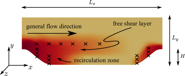
Figure 1: Domain shape for the flow over periodic hills. The $x$-, $y$- and $z$-coordinates are aligned with streamwise, wall-normal and spanwise directions, respectively. All dimensions are normalized with $H$ with $L_{x}/H=9$, $L_{y}/H=3.036$. The contour shows the variance field $\sigma(x)$, where darker color represents the larger variance. The locations where velocities are observed are indicated as crosses ($\times$).

2.2 Representations of Prior Knowledge in the Modeling Framework

In light of the prior knowledge presented above and based on the existing methods in the literature [11, 17, 19], we make the following modeling choices to represent the prior knowledge.

2.2.1 Composite model

The true Reynolds stress $\boldsymbol{\tau}$ is modeled as a random field of symmetric tensors with $\tilde{\boldsymbol{\tau}}^{rans}$ as its deterministic mean field, where $\tilde{\boldsymbol{\tau}}^{rans}$ is the Reynolds stress field given in the baseline RANS simulation whose model-form uncertainty is to be quantified.

2.2.2 Physical realizability of Reynolds stresses

To ensure physical realizability of its realizations, the value of the Reynolds stress field $\boldsymbol{\tau}$ at any given location $x$ is projected onto a space with six physically meaningful dimensions via the following eigen-decomposition [17, 14]:

$$\boldsymbol{\tau}=2k\left(\frac{1}{3}\mathbf{I}+\mathbf{a}\right)=2k\left(\frac{1}{3}\mathbf{I}+\mathbf{V}\Lambda\mathbf{V}^{T}\right)$$ (1)

where $k$ is the turbulent kinetic energy, $\mathbf{I}$ is the second order unit tensor, $\mathbf{a}$ is the anisotropy tensor, $\mathbf{V}=[\mathbf{v}_{1},\mathbf{v}_{2},\mathbf{v}_{3}]$, and $\Lambda=\textrm{diag}[\lambda_{1},\lambda_{2},\lambda_{3}]$ are its orthonormal eigenvectors and eigenvalues, respectively, with $\lambda_{1}+\lambda_{2}+\lambda_{3}=0$. This decomposition transforms the Reynolds stress to a space represented by six variables with clear physical interpretations: magnitude (represented by the turbulent kinetic energy $k$, which must be non-negative), shape (represented by two scalars $\lambda_{1}$, $\lambda_{2}$), and orientation (represented by three mutually orthonormal vectors $\mathbf{v}_{1}$, $\mathbf{v}_{2}$, and $\mathbf{v}_{3}$) of the Reynolds stress tensor [28, 14]. Further, $\lambda_{1}$, $\lambda_{2}$, and $\lambda_{3}$ are transformed to the Barycentric coordinates ($C_{1}$, $C_{2}$, $C_{3}$), with $C_{1}+C_{2}+C_{3}=1$, and subsequently to the natural coordinates ($\xi$, $\eta$). With the mapping from Barycentric coordinates to natural coordinates (see Fig. 2), the physically realizable turbulent stresses enclosed in the Barycentric triangle (panel a) are transformed to a square (panel b), i.e., $\{(\xi,\eta)\,|\,\xi\in[-1,1],\eta\in[-1,1]\}$, which is more convenient for parameterization. Details of the mapping are presented in A. In summary, we transform the Reynolds stress tensor to six physical dimensions denoted as $(k,\xi,\eta,\mathbf{v}_{1},\mathbf{v}_{2},\mathbf{v}_{3})$. All mappings involved are linear and invertible except for a trivial singular point in $(C_{1},C_{2},C_{3})\mapsto(\xi,\eta)$.

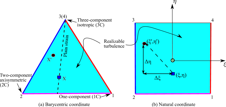
Figure 2: Mapping between Barycentric coordinates and natural coordinates, transforming the Barycentric triangle that encloses all physically realizable states [28, 16] to a square via standard finite element shape functions (detailed in A). Corresponding edges in the two coordinates are indicated with matching colors. The singular point 3(4) in the Barycentric coordinate, which maps to the edge 3–4 in the natural coordinate, does not pose any practical difficulties.

After the mapping of Reynolds stress $\tilde{\boldsymbol{\tau}}^{rans}$ to the physically meaningful dimensions, i.e., $k$, $\xi$, $\eta$, uncertainties are injected to the projected space on these variables. This is achieved by modeling the corresponding truths $k(x)$, $\xi(x)$, and $\eta(x)$ as random fields with $\tilde{k}^{rans}(x)$, $\tilde{\xi}^{rans}(x)$, and $\tilde{\eta}^{rans}(x)$ as priors. Specifically,

$$\log k(x) =\log\tilde{k}^{rans}(x)+\delta^{k}(x)$$ (2a)

$$\xi(x) =\tilde{\xi}^{rans}(x)+\delta^{\xi}(x)$$ (2b)

$$\eta(x) =\tilde{\eta}^{rans}(x)+\delta^{\eta}(x)$$ (2c)

where the spatial coordinate $x$ is the index of the random fields. Note that the logarithmic discrepancy of the turbulent kinetic energy $k$ is modeled in Eq. (2a) to ensure the non-negativity of $k$.

The realizability in this framework is ensured by bounding the perturbed anisotropy ($\eta$, $\xi$) within the square $[-1,1]\times[-1,1]$ in the $\xi$–$\eta$ plane as shown in Fig. 2b. Any perturbed state outside this range will be bounded to the edge of the square, which is admittedly an ad hoc modeling choice. As a result, the prior may become non-Gaussian and the perturbation sample may deviate from zero-mean if a large number of perturbations are bounded. However, note that for a Gaussian prior the percentage of out-of-bound points can be estimated, and thus the variance of the perturbation can be controlled straightforwardly given an allowable ratio of out-of-bound points. This is one of the advantages of mapping the Barycentric triangle to the square before introducing perturbation as opposed to directly perturbing the baseline within the Barycentric triangle.

The bounding scheme for ensuring realizability can distort the distribution of the sampled Reynolds stresses from the specified prior. Specifically, when the baseline Reynolds stresses are located near the realizability boundaries, e.g., the top vertex of the Barycentric triangle for points near walls, the bounding can cause the sample distribution to become truncated Gaussian. However, note that the tail truncation and the associated probability mass concentration near the boundaries are caused by the bounding procedure to ensure realizability, regardless of whether Barycentric coordinates or natural coordinates are used. This issue is further investigated in two follow-on studies [29, 30], where we proposed a random matrix approach which directly samples a maximum entropy distribution defined on the set of positive semidefinite matrices, and the artificial probability mass concentration described above is avoided. However, note that the approximate Bayesian inference method (i.e., the ensemble Kalman method) used in this work is not sensitive to the prior. From a practical point of view, the prior can be alternatively interpreted as an “initial guess” used in optimization [e.g., 24].

Perturbing the orientations of the modeled Reynolds stress tensor can potentially cause instability in the RANS momentum equation. Consistent with the work of Iaccarino et al., we focus on the magnitude ($k$) and the shape ($\lambda_{1}$ and $\lambda_{2}$, or equivalently the natural coordinates $\xi$ and $\eta$) of the Reynolds stress tensor $\boldsymbol{\tau}$, and do not introduce uncertainties into the orientations ($\mathbf{v}_{1},\mathbf{v}_{2},\mathbf{v}_{3}$). Consequently, the assumed uncertainty space of Reynolds stresses may not contain the truth because the true Reynolds stresses are likely to have different orientations from those of the RANS predictions. The implications of this fact will be further discussed in Section 4.1.2.

2.2.3 Spatial smoothness of Reynolds stress distribution

To ensure spatial smoothness and to reduce the dimension of the uncertainty space, the random fields to be inferred, i.e., $\delta^{k}$, $\delta^{\xi}$, and $\delta^{\eta}$, are projected to a deterministic functional basis set {$\phi_{i}(x)$}. That is,

$$\delta^{k}(x,\theta^{k})=\sum_{i=1}^{\infty}\omega^{k}_{i}|_{\theta^{k}}\;\phi_{i}(x)$$ (3a)

$$\delta^{\xi}(x,\theta^{\xi})=\sum_{i=1}^{\infty}\omega^{\xi}_{i}|_{\theta^{\xi}}\;\phi_{i}(x)$$ (3b)

$$\delta^{\eta}(x,\theta^{\eta})=\sum_{i=1}^{\infty}\omega^{\eta}_{i}|_{\theta^{\eta}}\;\phi_{i}(x)$$ (3c)

where the coefficients of the $i^{th}$ mode $\omega^{k}_{i}$, $\omega^{\xi}_{i}$, and $\omega^{\eta}_{i}$ are random variables depending on the realized outcome of $\theta^{k}$, $\theta^{\xi}$, and $\theta^{\eta}$, respectively, and $\phi_{i}(x)$ are deterministic spatial basis functions. An orthogonal basis set is chosen in this work as will be detailed below, but the orthogonality is not mandatory.

Remarks: The mapping in Section 2.2.2 involves linear transformation of the Reynolds stress at a given point to physical variables, which ensures the physical realizability of the Reynolds stresses in the prior. The orthogonal projection in Section 2.2.3 aims to represent the spatial distribution function on a basis set in a compact manner, which ensures spatial smoothness and reduces the uncertainty dimensions of $\boldsymbol{\tau}(x)$.

2.2.4 Representation of problem-specific prior knowledge

Finally, problem-specific knowledge is encoded in the choice of basis set {$\phi_{i}$}. Here we will use the flow over periodic hills as example to illustrate the representation of the problem-specific prior knowledge.

We model the prior of the discrepancies $\delta^{k}$, $\delta^{\xi}$ and $\delta^{\eta}$ as zero-mean Gaussian random fields (also known as Gaussian processes) $\mathcal{GP}(0,K)$, where

$$K(x,x^{\prime})=\sigma(x)\sigma(x^{\prime})\exp\left(-\frac{|x-x^{\prime}|^{2}}{l^{2}}\right)$$ (4)

is the kernel indicating the covariance at two locations $x$ and $x^{\prime}$. The variance $\sigma(x)$ is a spatially varying field specified (see the flood contour in Fig. 1) to reflect the prior knowledge that large discrepancies in modeled Reynolds stress are expected in certain regions. The correlation length scale $l$ can be specified based on the local turbulence length scale, but is taken as constant in this work for simplicity.

The orthogonal basis functions $\phi_{i}(x)$ in Eq. (3) take the form ${\phi}_{i}(x)=\sqrt{\hat{\lambda}_{i}}\hat{\phi}_{i}(x)$, where $\hat{\lambda}_{i}$ and $\hat{\phi}_{i}(x)$ are eigenvalues and eigenfunctions, respectively, of the kernel $K$ in Eq. (4) computed from the Fredholm integral equation [31]:

$$\int K(x,x^{\prime})\hat{\phi}(x^{\prime})\,dx^{\prime}=\hat{\lambda}\hat{\phi}(x)\,.$$ (5)

With this choice of basis set the expansions in Eq. (3) for the fields $\delta^{k}$, $\delta^{\xi}$ and $\delta^{\eta}$ become Karhunen–Loeve (KL) expansions [31], such that $\omega^{k}_{i}$, $\omega^{\xi}_{i}$, and $\omega^{\eta}_{i}$ are uncorrelated random variables with zero means and unit variances.

Remarks

The Gaussian process and KL expansions are intentionally presented in this Section to emphasize the fact that they are our specific choices for this problem and prior knowledge only. The optimal choice of basis set depends on the specific characteristics (e.g., smoothness, compactness of support) of the prior. Other functional basis sets, including wavelets [32] or radial basis functions [33], will be explored in future work.

2.3 Inverse modeling based on an iterative ensemble Kalman method

After the transformations above, the Reynolds stress random field $\boldsymbol{\tau}(x)$ is parameterized by the coefficients $\omega^{k}_{i}$, $\omega^{\xi}_{i}$, and $\omega^{\eta}_{i}$ in Eq. (3), which are truncated to $m$ modes and written in a stacked vector form as follows:

$$\boldsymbol{\omega}\equiv[\omega^{k}_{1},\,\omega^{\xi}_{1},\,\omega^{\eta}_{1},\;\omega^{k}_{2},\,\omega^{\xi}_{2},\,\omega^{\eta}_{2},\;\cdots,\;\omega^{k}_{m},\,\omega^{\xi}_{m},\,\omega^{\eta}_{m}]$$ (6)

We employ an iterative, ensemble-based Bayesian inference method [34] to combine the prior knowledge as represented above and the available data to infer the distribution of $\boldsymbol{\omega}$. This method is closely related to ensemble filtering methods (e.g., ensemble Kalman filtering), which are a class of standard data assimilation techniques commonly used in numerical weather forecasting [35]. An overview of the ensemble Kalman method based inverse modeling procedure is presented in Fig. 3. In the iterative ensemble method, the state of the system $\mathbf{x}$ is defined to include both the physical variables (i.e., velocity field $\mathbf{u}$) and the unknown coefficients $\boldsymbol{\omega}$, i.e., $\mathbf{x}\equiv[\mathbf{u},\boldsymbol{\omega}]^{T}$. This is called “state augmentation” [34]. One starts with an ensemble of states $\{\mathbf{x}_{j}\}_{j=1}^{N}$ drawn from their prior distributions. During each iteration, all samples in the ensemble are updated to incorporate the observations through the following procedure:

1. reconstruction of Reynolds stresses from the coefficients $\boldsymbol{\omega}$,

2. computation of velocity fields from the given Reynolds stress fields by solving the RANS equations (implemented as forward model tauFoam, detailed in Section 3), and

3. a Kalman filtering procedure to assimilate the velocity observation data to the computed states, leading to an updated ensemble.

The updating procedure is repeated until the ensemble is statistically converged. The convergence is achieved when the two-norm of the misfit between the predictions and the observations falls below the noises level of the observations [34]. The converged ensemble is considered a sample-based representation of the posterior distribution of the system state, from which the mean, variance, and higher moments can be computed. The algorithm of the inversion scheme is presented in B, and further details can be found in [34].

The noises added to the observations represent a combination of measurement errors and process errors [36]. The former is likely to be negligible for DNS data. However, the latter can be significant and is used to account for the fact that the observed system and the system described in the numerical model can have different dynamics. From a Bayesian perspective, adding the process noise allows the likelihood and the prior distribution to have overlap in their supports and thus be able to reconcile with each other in the inference procedure. As long as the chosen noise level $\sigma_{obs}$ is larger than a threshold (1% of truth in this work), the inferred posterior means are not sensitive to this parameter. See further discussion in [e.g., 34].

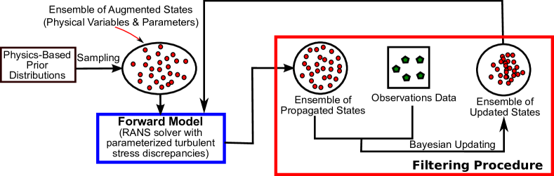
Figure 3: Inference of coefficients in the parameterized model discrepancies (e.g., discrepancies in RANS modeled Reynolds stresses) using an iterative ensemble Kalman inversion method. This approach combines prior knowledge of a given problem and available data to quantify and reduce model-form uncertainty.

An important property of the iterative ensemble Kalman method is that the posterior ensembles and its mean all lie in the linear space $\mathcal{A}$ spanned by the prior ensemble $\{\mathbf{x}_{j}\}_{j=1}^{N}$. In essence, this scheme attempts to search the space $\mathcal{A}$ to find the optimal solution that minimizes the misfit between the posterior mean and the observations, accounting for the uncertainties in both [34]. As with many inverse problems, this problem is intrinsically ill-posed. Specifically, because of the sparseness of the observation (the scenario of concern in our work), the amount of data is usually not sufficient to constrain the uncertainties in the states, which include the model discrepancies as components. The forward model essentially provides the regularization of the ill-posedness with its physical representation of the system dynamics.

The ensemble Kalman-based uncertainty quantification scheme used here is an approximate Bayesian method, and is computationally cheaper than the exact Bayesian scheme based on Markov Chain Monte Carlo sampling. It is not expected to give posterior distributions with comparable accuracy to those obtained from exact Bayesian schemes [37]. This limitation will be further discussed in Section 5.

2.4 Summary of the algorithm in the proposed framework

In summary, the overall algorithm of the proposed framework for quantifying and reducing uncertainties in a RANS simulation is presented as follows.

1. Perform the baseline RANS simulation to obtain the velocity $\tilde{\boldsymbol{u}}^{rans}(x)$ and Reynolds stress $\tilde{\boldsymbol{\tau}}^{rans}(x)$.

2. Perform the transformation $\tilde{\boldsymbol{\tau}}^{rans}\mapsto(\tilde{k}^{rans},\,\tilde{\xi}^{rans},\,\tilde{\eta}^{rans})$.

3. Compute KL expansion to obtain basis set $\{\phi_{i}(x)\}_{i=1}^{m}$, where $m$ is the number of modes retained.

4. Generate initial prior ensemble of coefficient vectors $\{\boldsymbol{\omega}_{j}\}_{j=1}^{N}$, where $N$ is the ensemble size.

5. Use iterative scheme shown in Fig. 3 to obtain the posterior ensemble of the state distribution. Specifically, in each iteration do the following:

   1. Recover the discrepancy fields $\delta^{k}$, $\delta^{\xi}$, and $\delta^{\eta}$ from the coefficient $\{\boldsymbol{\omega}_{j}\}_{j=1}^{N}$ in the current state and the basis functions via Eq. (3), and obtain realizations of $k$, $\xi$, and $\eta$ from Eq. (2) for each sample in the ensemble.

   2. Obtain Reynolds stress ensembles $\{\boldsymbol{\tau}_{j}\}_{j=1}^{N}$ via mapping $(k,\xi,\eta)\mapsto\boldsymbol{\tau}$.

   3. For each sample in the ensemble $\{\boldsymbol{\tau}_{j}\}_{j=1}^{N}$, solve the RANS equations for velocity field $\boldsymbol{u}_{j}$ with given Reynolds stress field $\boldsymbol{\tau}_{j}$.

   4. Compare the ensemble mean with velocity observations, and use the Kalman filtering procedure to correct the augmented system state ensemble $\{\mathbf{x}_{j}\}_{j=1}^{N}$, where $\mathbf{x}_{j}=[\mathbf{u}_{j},\boldsymbol{\omega}_{j}]^{T}$. The updated coefficient vector ensemble $\boldsymbol{\omega}_{j}$ is thus obtained as part of the system state ensemble.

   5. Stop if statistical convergence of the ensemble as defined in Section 2.3 is achieved.

3 Implementation and Numerical Methods

The uncertainty quantification framework including the mapping of Reynolds stresses and the iterative ensemble Kalman method is implemented in Python, which interfaces with RANS models and the KL expansion procedures to form the complete framework. The package UQTk developed by Sandia National Laboratories is used to perform the KL expansions [38]. Two types of RANS solvers are used in this framework, a conventional baseline RANS solver simpleFoam and a forward RANS solver tauFoam which computes velocity field with a given Reynolds stress field. Both solvers are described as below.

The baseline simulation uses a built-in RANS solver simpleFoam in OpenFOAM for incompressible, steady-state turbulent flow simulations. OpenFOAM (for “Open source Field Operation And Manipulation”) is an open-source, general-purpose CFD platform based on finite-volume discretization. The platform consists of a wide range of solvers and post-processing utilities. The SIMPLE (Semi-Implicit Method for Pressure Linked Equations) algorithm [39] is used to solve the coupled momentum and pressure equations. Collocated grids are used, and the Rhie and Chow interpolation is used to prevent the pressure–velocity decoupling [40]. Second-order spatial discretization schemes are used to solve the equations on an unstructured, body-fitting mesh. Given the specification of the flow including initial conditions (to start the iteration), boundary conditions, geometry, and the choice of turbulence model, the simpleFoam solver computes the velocity field along with Reynolds stresses by solving the RANS equations as well as the equations for the turbulence quantities (e.g., turbulent kinetic energy $k$ and the rate of dissipation $\varepsilon$ for $k$–$\varepsilon$ models). We choose the Launder–Sharma low Reynolds number $k$–$\varepsilon$ model [41] in the baseline simulations. Accordingly, the meshes are refined wall-normal direction near the wall to resolve the boundary layer. This is to avoid the complexity of using wall-functions, which is in consistent with the work of Emory et al. [17]. As can be seen in the overall algorithm presented in Section 2.4, for each uncertainty quantification case the baseline simulation is performed only once.

The forward RANS model tauFoam is invoked repeatedly in the Bayesian inference procedure. This solver is adopted from and similar to simpleFoam except that it computes the velocity directly with a given Reynolds stress field. There is no need to specify a turbulence model and or to solve the equations for turbulence quantities, since the Reynolds stress is given. Moreover, as the forward RANS simulations are initialized with the converged baseline solutions, the number of iterations needed to achieve convergence is much smaller than that in the baseline simulation. As a result, the computational cost for each call of the forward RANS model tauFoam is much lower than that of the conventional RANS solver simpleFoam. In the simulations presented below, the forward RANS simulations need only 10% of the computational cost as that of the baseline simulation to achieve the same residual.

4 Numerical Simulations

Two canonical flows, the flow in a channel with periodic constrictions (periodic hills) and the fully developed turbulent flow in a square duct, are chosen to evaluate the performance of the proposed framework. The periodic hill flow features a recirculation zone formed by a forced separation, a strong mean flow curvature due to the domain geometry, and a shear layer that is not aligned with the overall flow direction. All these features are known to pose challenges for turbulence modeling. The square duct flow is characterized by a secondary flow pattern in the plane perpendicular to the main flow. The in-plane secondary flow is driven by the imbalance in the normal components of the Reynolds stress tensor, which cannot be captured by models with isotropic eddy viscosity turbulent models including most of the widely used models such as $k$–$\varepsilon$, $k$–$\omega$, and eddy viscosity transport models. The two challenging cases are chosen to demonstrate the capability of the proposed framework in quantifying and reducing uncertainties in the RANS model predictions by incorporating sparse observations.

4.1 Flow over Periodic Hills

4.1.1 Case setup

The periodic hill flow is widely used in the CFD community to evaluate the performance of turbulence models due to the availability of experimental and numerical benchmark data [42]. The geometry of the computational domain and the coordinate system are shown in Fig. 1. The Reynolds number based on the crest height $H$ and the bulk flow velocity $U_{b}$ at the crest is $Re_{b}=2800$. Periodic boundary conditions are applied in the streamwise ($x$) direction, and non-slip boundary conditions are applied at the walls. The mean flow is two-dimensional, and thus the spanwise ($z$) direction is not considered for the RANS simulations.

The mesh and computational parameters used in the uncertainty quantification procedure are presented in Table 1. Despite the coarse meshes, the walls are adequately resolved in both cases as required by the Lauder–Sharma turbulence model [41]. The distance between the center of the first cell and the wall is smaller than 1 in most regions for periodic hill case and 0.7 for the square duct case. Parameters of the meshes for both cases are shown in Table 1.

The uncertainties in $\xi$, $\eta$, $k$ are all considered, and thus $\delta^{\xi}$, $\delta^{\eta}$ and $\delta^{k}$ are all random fields. This choice is based on our prior knowledge that both the Reynolds stress anisotropy (indicated by the shape $\boldsymbol{\tau}$, or equivalently, $\xi$ and $\eta$) and turbulent kinetic energy $k$ predicted by the RANS model are biased, and both are important for the accurate prediction of the flow behavior. The length scale parameter $l$ is chosen according to the approximate length scale of the flow, which can be obtained either from our physical understanding of the flow or, if that is not available, from the baseline RANS simulation. Velocity observations are generated by adding Gaussian random noises with standard deviation $\sigma_{obs}$ to the truth from DNS data. Specifically, the observations used in each iteration are independent realizations from a Gaussian distribution whose mean is the truth and standard deviation $\sigma_{obs}$ is 10% of the true mean value. The noises at different locations are uncorrelated. The observation points are arranged so that they are closer in regions where the spatial changes of the flow are more rapid (the recirculation zone leeward of the hill and the reattached flow region windward of the hill), and are further apart in the free shear region downstream of the hill crest. This arrangement of observations is expected in actual experiments. The ensemble usually converges in approximately 10 iterations. For all cases presented in this work, 60 samples are used in the ensemble. We have performed detailed sensitivity studies on the ensemble size, and it was found that the inferred velocities and QoIs do not vary if more than 30 samples are used. This finding is consistent with earlier studies when EnKF was used in data assimilations in applications such as weather forecasting [43]. The computational cost of the proposed procedure is further discussed in Section 5.1.

The non-stationary Gaussian process models for $\delta^{\xi}$, $\delta^{\eta}$ and $\delta^{k}$ share the same variance field $\sigma(x)$, which are shown as flood contour in Fig. 1. Design of the variance field is strictly based on physical prior knowledge as described in Section 2.2.4, and does not take the DNS data into account, since the complete field of the true Reynolds stresses are rarely known in practical applications. Specifically, the variance fields of the priors as shown in Figs. 1 and 10 are constructed by superimposing a constant background value $\sigma_{0}$ and a spatially varying field $\sigma_{local}(x)$, i.e., $\sigma(x)=\sigma_{0}+\sigma_{local}(x)$. For the periodic hill case, the background $\sigma_{0}$ is set to be 0.2. To obtain the field $\sigma_{local}(x)$, we specify that $\sigma_{local}=0.5$ at the following locations, where RANS predictions are considered less reliable: (1) the hill crest, (2) the center of the recirculation region, (3) the windward side of the hill, and (4) the free-shear layer downstream the crest. Interpolations based on radial basis functions with exponential kernels are used to obtain $\sigma_{local}(x)$ at other locations. As such, its value decays to zero far away from the locations specified above. The length scale of the basis functions is estimated based on the characteristic length of the mean flows, which is chosen as the hill height $H$.

The first sixteen modes obtained from the KL expansion are used to reconstruct the discrepancy field. The number of modes retained is chosen such that the reconstructed field has at least 80% of the total variance of the original random field. A rule of thumb is that a coverage ratio of 80% is adequate for a faithful representation. Increasing the number of modes increases the difficulty of the inference and may lead to deteriorated results for a given amount of observation data.

Parameter sensitivity analysis has been conducted to ensure that reasonable variations of the computational parameters above do not lead to significantly different results or conclusions. In particular, we have shown in a follow-on study [44] that even in the complete absence of prior knowledge (i.e., a constant variance field $\sigma(x)$), the inferred velocities are still significantly improved, albeit slightly less so than that with an informative prior. Specifically, in the region near the upper wall, much more uncertainties are presented in the posterior ensemble when a non-informative, constant variance field is used.

Table 1: Mesh and computational parameters used in the flow over periodic hills and the flow in a square duct.

cases	periodic hill	square duct
mesh ($n_{x}\times n_{y}$)	$50\times 30$	$30\times 30$
domain size ($L_{x}\times L_{y}\times L_{z}$)	$9H\times 3.306H\times 0.1H$	$0.4D\times 0.5D\times 0.5D$
$\Delta x\times\Delta y\times\Delta z$ in $y^{+}$	$35\times[2,65]\times 850$	$24\times[1.4,30]\times[1.4,30]$
first grid point in $y^{+}$	$\sim 1$, below $2y^{+}$ in most region	0.7
number of samples $N$	60
fields with uncertainty	$\xi$, $\eta$, $k$	$\xi$, $\eta$
number of modes $m$ per field	$16$	$8$
length scale(a)	H	0.1D
number of observation	18	25(b)
std. dev. observation noise ($\sigma_{obs}$)	10% of truth

4.1.2 Results

The first six modes of the KL expansion are presented in Fig. 4 along with two typical realizations. This is to illustrate the uncertainty space of the Reynolds stress discrepancy field (or more precisely its projections $\delta^{\xi}$, $\delta^{\eta}$ and $\delta^{k}$) . All the modes have been shifted and normalized to the range $[0,1]$. It can be seen that in all the models and the realizations the variations mostly concentrate in the three pre-specified regions (recirculation zone, free shear region, and the reattached flow windward of the hill), and the upper part of the channel has rather small variations. This is consistent with our physical prior knowledge specified through the variance field design.

(a) mode 1

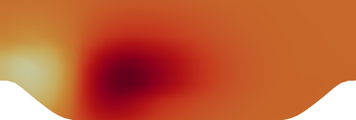
(b) mode 2

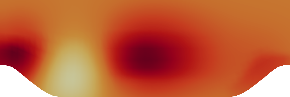
(c) mode 3

(d) mode 4

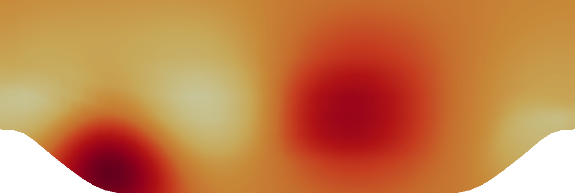
(e) mode 5

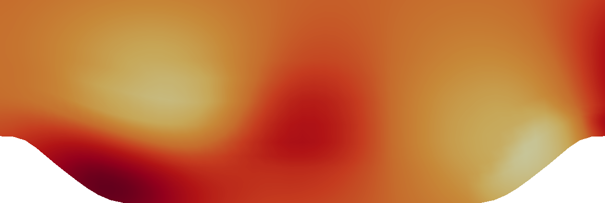
(f) mode 6

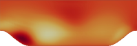
(g) realization 1

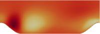
(h) realization 2

Figure 4: Illutstration of KL expansion modes of the periodic hill case. All the modes have been shifted and scaled into the range between 0 (lightest) and 1 (darkest) to facilitate presentation, and the legend is thus omitted. Panels (a) to (f) represent modes 1 to 6, respectively. Lower modes are more important. Panels (g) and (h) show the turbulent kinetic energy associated with two typical realizations of the Reynolds stress discrepancy fields.

Accurate predictions of the recirculation and the reattachment of the flow are of the most interest in the flow over periodic hills. Therefore, we identify three quantifies of interest for this case: (1) the velocity field, in particular the velocities in the recirculation zone and reattached flow region windward of the hill, (2) the distribution of shear stresses $\tau_{w}$ on the bottom wall, and (3) the reattachment point $x_{attach}$. Other quantities that are important in engineering design and analysis (e.g., friction drag, form drag, size of separation bubble) are closely related to the three QoIs above.

The prior and posterior ensembles of the velocities are presented in Fig. 5 with comparison to the DNS benchmark results. The geometry of the domain is also shown to facilitate visualization. From Fig. 5a it can be seen that the prior mean velocity profiles are very close to those from the baseline RANS simulation, with only minor differences at a few locations (e.g., near the bottom wall at $x/H=4$, 5, and 6). This is not surprising, since the Reynolds stresses prior ensemble use the RANS modeled Reynolds stress $\tilde{\boldsymbol{\tau}}^{rans}$ as the mean. In other words, the ensemble is obtained by introducing perturbations to the $\tilde{\boldsymbol{\tau}}^{rans}$. Therefore, the similarity between the velocity profiles in the baseline simulation and those of the prior ensemble indicates that the mapping from Reynolds stress to velocity is approximately linear with respect to the perturbations introduced to the prior Reynolds stresses ensemble. Clearly, both the baseline velocities and the prior mean velocities deviate significantly from the benchmark results, particularly in the recirculation region (leeward of the hill). From Fig. 5 it can be seen that the posterior ensemble mean of the velocities along all the lines are significantly improved compared to the baseline results.

The remaining differences between the obtained posterior mean and the benchmark data can be attributed to two sources: (1) the sparseness of the observation data, and (2) the inadequacy of the proposed inference model, specifically, the posterior mean Reynolds stress does not reside in the space $\mathcal{A}$ spanned by the prior ensemble. However, note that obtaining the correct Reynolds stresses is a sufficient but not necessary condition to infer the correct velocities. For example, if the divergence of the true Reynolds stresses resides in the space spanned by the prior ensemble, the true mean velocity can still be obtained. This is not surprising since it is the divergence of the Reynolds stress tensor field that appears as source term in the RANS momentum equation. To illustrate this point, it is particularly interesting to investigate the scenario when large amounts of data are available, since any remaining discrepancies should then be explained solely by the inadequacy of the inference processes. We performed an experiment where all the benchmark velocities along ten sampled lines at $x/H=0,0.5,1,2,\cdots,8$ were used as observations. In this scenario the posterior mean velocities agree with the benchmark data very well, even in the regions between the sample lines, where no data are available. However, significant discrepancies still remain between the inferred posterior mean of the Reynolds stresses and the benchmark. We argue that the inability to obtain the correct Reynolds stress field is not an intrinsic limitation of the proposed method. Rather, it can be explained by the non-unique mapping between Reynolds stress and velocities as described by the RANS equations. That is, two distinctly different Reynolds stress fields can lead to identical or very similar velocity fields, because the divergence of the Reynolds stress appears in the RANS equation as pointed out above. The non-unique mapping is further discussed in Section 5.3. However, when we assume that some sparse measurements of Reynolds stresses are available, which admittedly are difficult to obtain in practical experiments, the inferred Reynolds stresses did improve significantly. The results are omitted here for brevity.

In order to obtain the true Reynolds stresses, the posterior mean Reynolds stress must reside in the space $\mathcal{A}$ spanned by the prior ensemble, but in practical inferences there is no guarantee this will be the case. There are two reasons for this. First, uncertainties are only introduced to the magnitude ($k$) and shape ($\xi$ and $\eta$) of the baseline Reynolds stresses, and not to the orientations ($\mathbf{v}_{1}$, $\mathbf{v}_{2}$, and $\mathbf{v}_{3}$). Second, a limited number of modes are retained in the KL expansion, which correspond to very smooth fields of Reynolds stress discrepancies. Therefore, if we think of the true Reynolds stress as residing in a high-dimensional space, in the current framework we assume that the truth is reasonably close to the baseline prediction $\tilde{\boldsymbol{\tau}}^{rans}$, and thus we only search the vicinity of $\tilde{\boldsymbol{\tau}}^{rans}$ for realizable candidates. This is justified by the confidence that the chosen baseline RANS model is rather capable, usually backed by previous experiences accumulated by the community on the model of concern.

Finally, we emphasize that if the true Reynolds stresses do reside in the space spanned by the prior ensemble, the posterior mean velocity and the Reynolds stresses would indeed coincide with the truths. This scenario could occur if the baseline Reynolds stress $\tilde{\boldsymbol{\tau}}^{rans}$ only differs from the true Reynolds stress in magnitude $k$ and shape $\xi$ and $\eta$, and the discrepancy is smooth enough to be represented by the chosen number of modes. However, both scenarios are rather unlikely in any nontrivial cases. For verification purposes we have designed a case of flow over periodic hills with synthetic data (as opposed to DNS data) that satisfies the requirements above, and have confirmed that the obtained posterior mean velocity indeed exactly agrees with the truth in this case, and that the true Reynolds stress can also be obtained. The results are detailed in a separate work [44].

This claim that the prior has small influence to the prior is apparently contradictory to the Bayesian inference theory, which states that the posterior is proportional to the product of the prior and the likelihood informed by the observation data. However, in the ensemble Kalman method used in this work, the observation data are imposed on the prior iteratively (albeit with different noises in each iteration). As a result, the influence of the prior on the posterior diminishes as the posterior proceeds to statistical convergence. From a practical perspective, the iterative ensemble Kalman method can also be interpreted as an optimization procedure (e.g., that used by Parish et al. [24]), with the prior corresponding to the initial guess. This interpretation, as an alternative to the Bayesian interpretation, has been advocated in the literature [34, 45].

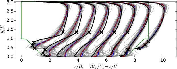
(a) Prior velocities ensemble

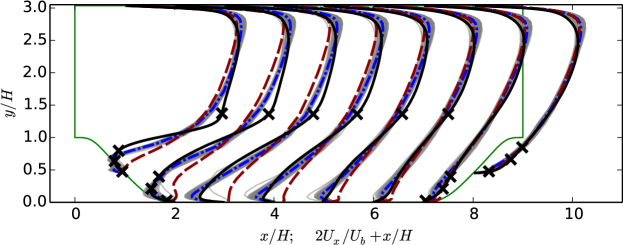
(b) Posterior velocities ensemble

Figure 5: The prior and posterior ensembles of velocity profile for the flow over periodic hill at eight locations $x/H=1,\cdots,8$ compared with benchmark data and baseline results. The locations where velocities are observed are indicated with crosses ($\times$).

Figure 6 shows the 95% credible intervals estimated from the data in the prior and posterior velocity ensembles. That is, at each point, 95% of the samples fall within the shaded region (light/pink shaded for the prior and dark/blue shaded for the posterior). Note that the credible intervals shown here are point estimations and do not contain information on the spatial correlations of the velocity profiles. It can be seen from Fig. 6 that the 95% credible interval in the posterior is significantly narrowed compared to that in the prior, which suggests that the model form uncertainty is reduced by incorporating the velocity observation data. Such a reduction of uncertainty is more visible in the recirculation zone, where more observation data are available. In contrast, the prior uncertainty near the upper wall largely remains, which is due to the lack of observation data in this region.

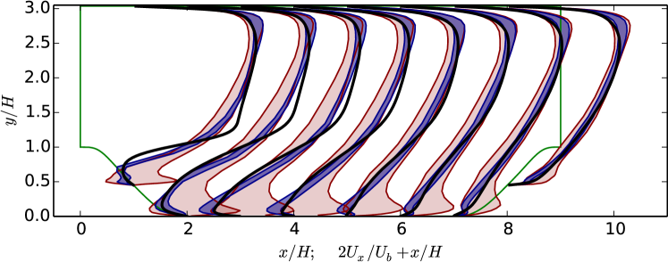
Figure 6: The 95% credible intervals of the prior (light/pink shaded region) and posterior (dark/blue shaded region) ensembles of velocity profiles for the flow over periodic hills.

The other two QoIs, bottom wall shear stress $\tau_{w}$ and the reattachment point $x_{attach}$, are shown in Fig. 7. Similar to the velocity profiles in Fig. 5, both prior and posterior ensembles are presented and compared with benchmark data and baseline results. It can be seen from Fig. 7a that the prior ensemble means of both $\tau_{w}$ and $x_{attach}$ deviate from the benchmark DNS data significantly. In particular, the baseline RANS simulation predicts a much smaller recirculation zone than the truth. Figure 7b shows that in most of the region (between $x/H=1$ and $x/H=8$) the posterior ensemble mean has better agreement with the DNS data than the baseline results. In fact, in this region, all samples in the posterior ensemble have better agreement with the benchmark than the baseline results in terms of both wall shear stress and reattachment point. This improvement demonstrates the merits of the current framework. Incorporating observation data and physical prior knowledge indeed leads to improved predictions of both QoIs.

It is noted that in the immediate vicinity of the hill crest, i.e., near $x/H=0.5$ and $x/H=8.5$, the posterior ensemble is similar to or even slightly deteriorated compared to the baseline in terms of agreement with DNS data. The reason is that in this region the flow has rapid spatial variations. Specifically, there is a separation between $0<x/H<1$, and a large mean flow curvature with strong pressure gradient between $8<x/H<9$. Consequently, the length scales of the coherent structures in this region are small, and thus the correlations between this part of the flow and other regions are weak. On the other hand, no velocity observations are available in this region. Here we point out an important fact that the Bayesian inference based on ensemble Kalman method primarily relies on the correlation between the predicted system state variables at different locations to make corrections. Specifically, the observations only bring information to the states at the locations correlated to the observed states. Hence, poor prediction is expected for a region that has neither observations within it nor statistically significant correlations with the regions that have observations. The role of correlation in the current framework is further discussed in Section 5.2.

The prior and posterior distributions of the reattachment point represented by samples are shown in Fig. 7 (bottom panels). It can be seen that the bias in the prior distribution as compared to the DNS data is large, while in the posterior distribution the bias is significantly corrected. Moreover, the prior sample scattering is wide, indicating large uncertainties. In contrast, the posterior distribution is significantly narrowed, which indicates increased confidence in the prediction by incorporating velocity observations into the Bayesian inference.

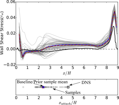
(a) Prior ensemble

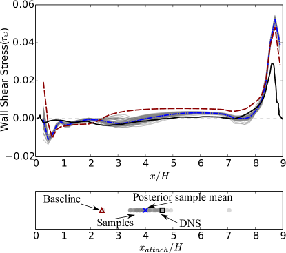
(b) Posterior ensemble

Figure 7: (a) Prior ensemble and (b) posterior ensemble of the bottom wall shear stress $\tau_{w}$ (top panels) and reattachment point $x_{attach}$ (bottom panels) for the flow over periodic hills. The region with negative shear stress $\tau_{w}$ indicates the extent of recirculation zone on the bottom wall. The reattachment point is the downstream end of the recirculation zone, which can be determined by the location at which the wall shear stress changes from negative to positive. Note that certain samples in the ensemble have two recirculation zones that are very close to each other. In these cases the reattachment point of the downstream one is taken.

The comparison of 95% credible interval obtained from the prior and posterior ensemble of wall shear stresses are presented in Figure 8. Similar reduction of model-form uncertainty as shown in Fig. 6 is observed here. Compared to that in the prior, the 95% credible interval in the posterior has a much smaller uncertainty and a better coverage of the benchmark data in the region between $x/H=1$ and 5. This is because there are more observations available in the vicinity. Admittedly, in some regions, e.g., between $0<x/H<1$ and $8<x/H<9$, the posterior credible interval does not improve or even deteriorate compared to the prior, which is due to the lack of observation data and the relatively small length scale in these regions as discussed above. It is noted that in some regions the 95% credit intervals, e.g., in Figs. 6 and 8, failed to cover the truth, which indicates that the current method should still be used with caution when making high-consequence decisions. The iterative ensemble Kalman method tends to underestimate uncertainties in the posterior distributions, a difficulty shared by many other maximum likelihood estimators as well [46].

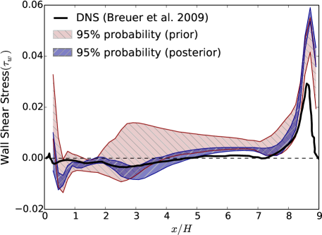
Figure 8: The 95% credible intervals of the prior (light/pink shaded region) and posterior (dark/blue shaded region) ensembles of bottom wall shear stress for the flow over periodic hills.

Figure 9 shows that the bias in the turbulent kinetic energy (TKE) from baseline RANS prediction has been partly corrected, especially for the upstream region. It is possible that the production of TKE due to the instability in the free-shear region after the separation is the driving factor. Consequently, the improved prediction of TKE in this region leads to the corrections for the velocities and other QoIs in the entire field. However, note that the posterior mean of TKE is not necessarily better than the baseline results at all locations. The TKE levels immediately downstream of the hill crest have been increased, but at the downstream locations the posterior mean are not significantly better than the baseline. In the process of minimizing misfit with the observations, some compromises are inevitably made, with some regions such as the upstream experiencing more corrections than other regions such as the downstream region. A possible explanation is that the TKE in the free-shear region has stronger correlations with the velocities at the observed locations. However, it is also possible that the TKE does not necessarily need to be improved to provide better velocity field due to the non-unique mapping from Reynolds stress field to velocity field, as has been discussed above. More detailed discussion can be found in Section 5.3.

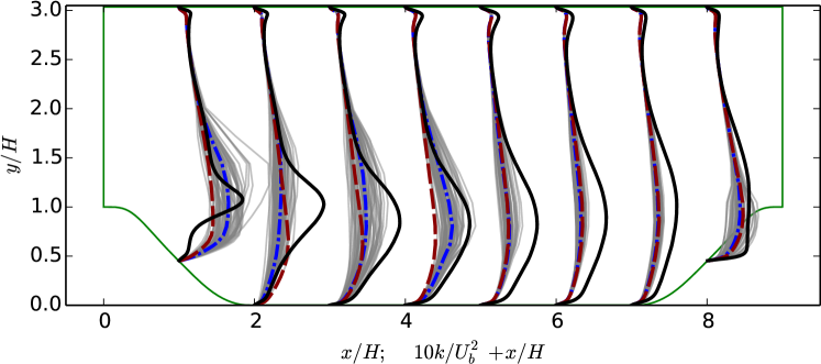
(a)

Figure 9: Posterior ensemble of the turbulent kinetic energy $k$ with its mean compared to the baseline results and the benchmark DNS data. The prior ensemble is omitted for $k$, since its mean is the same as the baseline prediction.

4.2 Fully Developed Turbulent Flow in a Square Duct

4.2.1 Case setup

The fully developed turbulent flow in a square duct is a widely known case for which many turbulence models fail to predict the secondary flow induced by the Reynolds stresses. The geometry of the case is shown in Fig. 10. The Reynolds number based on the edge length $D$ of the square and the bulk velocity $U_{b}$ is $Re_{b}=10320$. All lengths presented below are normalized by the height $h$ of the computational domain, which is half of $D$. Extensive benchmark data from DNS are available in the literature [47, 48].

Standard computational setup as used in the literature is adopted in this work. Only one quadrant of the physical domain is simulated considering the symmetry of the flow with respect to the centerlines along $y$- and $z$-axes as indicated in Fig. 10. We emphasize here that our study is concerned with the mean flow, since the objective is to quantify the uncertainties in RANS simulations. The instantaneous flows are beyond the scope of our discussions, and they do not have the symmetries mentioned here. Non-slip boundary conditions are imposed at the walls and symmetry boundary conditions (zero in-plane velocities) are applied on the symmetry planes. Theoretically, one can further reduce the computational domain size to 1/8 of the physical domain by utilizing the symmetry with respect to the square diagonal. However, this symmetry is not exploited, as it would be difficult to impose proper boundary conditions on the diagonal. The symmetry in the baseline RANS simulation results is implied by the diagonal symmetry of the geometry and boundary conditions. When conducting forward RANS simulations with given Reynolds stress fields, caution must be exercised to ensure that the perturbations introduced to $\tilde{\boldsymbol{\tau}}^{rans}$ have diagonal symmetry, which will be discussed later. Otherwise, the posterior velocities may be asymmetric with respective to the diagonal.

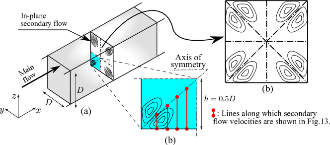
Figure 10: (a) Schematic for the fully developed turbulent flow in a square duct. The $x$ axis is aligned with the streamwise direction. Secondary flows exist in the $y$–$z$ plane, which are schematically represented with contours. (b) Symmetry of the (mean) flow with respect to the centerlines in $y$- and $z$-directions and along the diagonals. (c) The computational domain covers only a quarter of the physical domain due to the centerline symmetry. The cross-sections along which QoIs (e.g., velocities and Reynolds stress imbalance) are compared to benchmark data are also indicated.

The mesh and computational parameters for this case are shown in Table 1. Choice of parameters can be motivated similarly as in the periodic hill case. A notable difference is that only uncertainties in the shape of the Reynolds stress (i.e., $\xi$ and $\eta$) are considered in the square duct flow case. The QoI for this flow is the in-plane flow velocities, which are primarily driven by the normal stress imbalance $\tau_{yy}-\tau_{zz}$, a quantity that is associated with the shape of $\boldsymbol{\tau}$. The design of the variance field $\sigma$ is based on the same principle as in the periodic hill flow. Specifically, we chose $\sigma_{0}=0.2$ throughout the field and $\sigma_{local}=0.5$ at the lower left corner. The length scale of the radial basis kernel is chosen as 0.1D based on the estimation of length scale of secondary flow (see Table 1). It is known that RANS models have more difficulties in predicting the flow near the corner, which justifies the large value of $\sigma(x)$ near the corner and the gradual decrease away from the corner as well as towards the diagonal. Moreover, the variance field is chosen to be symmetric along the diagonal of the $y$–$z$ plane in consideration of the flow symmetry.

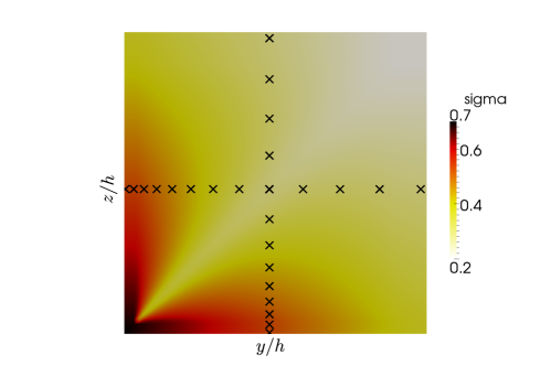
Figure 11: Contour of the variance field $\sigma(x)$ and locations of the observations for the square duct flow case. Larger variances are allowed near the corner due to the difficulties RANS models have in predicting the secondary flow in this region. The variance field is chosen to be symmetric along the diagonal of the $y$–$z$ plane in consideration of the flow symmetry.

4.2.2 Results

The first six modes of KL expansion are shown in Fig. 12 along with two typical realizations. All the modes have been shifted and normalized into the range $[0,1]$. Only the diagonally symmetric modes are retained to guarantee the symmetry of the Reynolds stress along the diagonal, which leads to the symmetry of the posterior velocities. The observations are obtained from the DNS data [47] by adding Gaussian random noises as in the periodic hill flow. Velocities are observed at 25 points as shown in Fig 10, half of which are distributed along the line $y/h=0.5$ and the other half along $z/h=0.5$. Note that half of the information from the observations is redundant due to the diagonal symmetry of the flow.

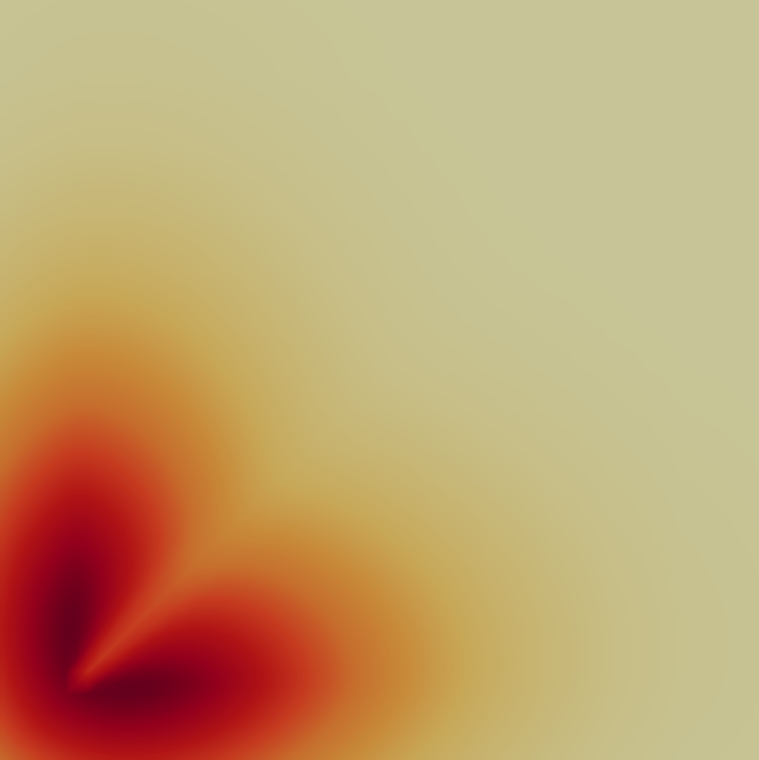
(a) mode1

(b) mode 2

(c) mode 3

(d) mode 4

(e) mode 5

(f) mode 6

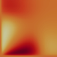
(g) realization 1

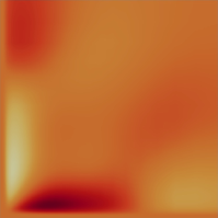
(h) realization 2

Figure 12: Illustration of KL expansion modes for the square duct flow case. All presented modes have been shifted and scaled into a range of 0 (lightest) to 1 (darkest) to facilitate presentation, and the legend is thus omitted. Panels (a) to (f) denote modes 1 to 6, respectively, with lower modes being more important. Only the modes with diagonal symmetry are retained to guarantee the symmetry of perturbed Reynolds stresses field. Panels (g) and (h) show the magnitude of Reynolds stress imbalance $|\tau_{yy}-\tau_{zz}|$ associated with two typical realizations of the discrepancy fields.

The ability of a numerical model to predict the secondary flow in $y$–$z$ plane is of most interest for the flow in square duct. Therefore, the in-plane velocity field is identified as the QoI for this case. The in-plane flow velocity ($U_{y}$) on the four cross-sections as indicated in Fig. 10 are presented to facilitate quantitative comparison with the baseline and benchmark results. The velocity profiles $U_{z}$ in the $z$ direction have similar characteristics as $U_{y}$ (but are not identical) and are thus omitted. The prior and posterior ensembles of the velocity profiles for $U_{y}$ are shown in Fig. 13. Only the velocity profiles in the region below the diagonal are presented due to the diagonal symmetry. It can be seen from Fig. 13 that the baseline RANS simulation predicts uniformly zero in-plane velocities as expected. Around the baseline prediction, the prior ensembles are scattered due to the perturbation of $\delta_{\xi}$ and $\delta_{\eta}$. The large range of scattering indicates that the secondary flow is sensitive to the anisotropy of Reynolds stresses tensor, which has been reported in previous studies [18, 47]. Compared to the prior ensemble mean and the baseline RANS prediction, the posterior ensemble mean of the velocities are significantly improved along all four cross sections, as shown by good agreements with the benchmark data. The scattering has been significantly reduced as well, while still covering the truth adequately in most regions. The remaining differences and the regions where the ensemble fails to cover the truth can be explained similarly as in the periodic hill case. Similar to that in the periodic hill case,

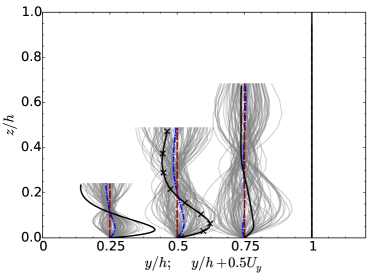
(a) Prior ensemble

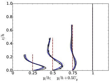
(b) Posterior ensemble

Figure 13: (a) Prior velocity ensemble and (b) posterior velocity ensemble at four spanwise locations $y/h=0.25,0.5,0.75$ and $1$ with comparison to baseline and benchmark results. The velocity $U_{z}$ in the $z$ direction have similar characteristics and are thus omitted. The velocity profiles in the prior ensemble are scaled by a factor of 0.3 for clarity.

Figure 14 shows a comparison of the posterior ensemble mean field of the in-plane flow velocity and the benchmark data. They are presented as vector plots to show the overall features of secondary flow and particularly the vortex structure. The length and direction of an arrow indicate the magnitude and direction, respectively, of the in-plane flow velocity at that location. The plots are arranged such that a perfect agreement between the two would show as exact symmetry of the two panels along the center line. The vector plot of the velocity field from the baseline RANS prediction is omitted since it is uniformly zero. It can be seen that the posterior ensemble mean demonstrates a very good agreement with the benchmark data in most aspects, i.e., the direction and the intensity of secondary flow at most locations as well as the center of vortex structure. Only minor differences between the two can be identified. For example, the posterior mean velocity has a slightly smaller gradient of velocity magnitude compared to the benchmark results near the symmetry line. The agreement clearly demonstrates the merits of the current framework, particularly considering the fact that most of the commonly used turbulence models are not capable of predicting the in-plane flow. Specifically, all isotropic eddy viscosity models completely miss the secondary flow, which is explained by the negligible $\partial{U_{y}}/\partial{y}$ and $\partial{U_{z}}/\partial{z}$ terms and the Boussinesq assumption that Reynolds stress is proportional to local strain rate of the mean flow. Even advanced models (e.g., Reynolds stress transport models) tend to underestimate the flow intensity [49]. Admittedly, velocity observations at some locations are used in this method, but the amount of data used in the inference is rather small compared to the total degrees of freedom of the Reynolds stress field.

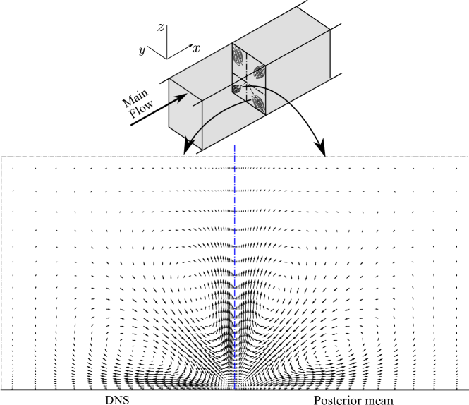
Figure 14: Comparison of the velocity field in a square duct between the posterior mean and benchmark DNS data.The length and direction of an arrow indicate the magnitude and direction, respectively, of the in-plane flow velocity. The plots are arranged such that a perfect agreement between the two would show as exact symmetry of the two panels along the vertical center line. The vector field from the baseline RANS prediction is omitted since it is uniformly zero.

As mentioned above, the normal stress imbalance $\tau_{yy}-\tau_{zz}$ is the main driving force of the secondary flow. Therefore, the prior and posterior ensembles of the imbalance at five locations, $y/h=0.25,0.5,0.6,0.75$, and $1$, are presented in Fig. 15. It can be seen that the baseline RANS prediction of $\tau_{yy}-\tau_{zz}$ is zero. Compared to the baseline RANS prediction, the posterior normal stress imbalance shows a significant improvement in regions close to the observations ($y/h=0.5$), although differences still exist, especially in the regions far away from the observations (e.g., at $y/h=1$). It is consistent with the argument made in Section 2.2.4 that the correlation decreases with distance, and that the quality of correction heavily depends on correlations. Note that the inferred stress imbalances at $y/h=0.75$ agree with the benchmark much better than do those at $y/h=0.25$, although they have approximately the same distances from the observations, which are distributed along $y/h=0.5$. This can be explained by the fact that the length scale of the flow decreases towards the corner (e.g., near $y/h=0.25$) due to the constriction of the duct walls, and thus the correlation decreases much faster in this region than near the symmetry line.

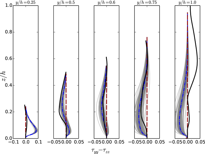
Figure 15: Comparison of the normal stresses imbalance at five locations $y/h=0.25,0.5,0.6,0.75$ and $1.0$. A larger horizontal axis range is used in the panel for $y/h=0.25$ due the large range of values $\tau_{yy}-\tau_{zz}$ at this location.

5 Discussion

5.1 Computational cost of the model-form uncertainty quantification

As mentioned in Sections 3. The ensemble Kalman method uses 60 samples (see Table 1) and needs approximately 10 iterations to achieve statistical convergence. Therefore, each uncertainty quantification case involves 600 evaluations of the forward RANS model tauFoam. Since each forward RANS evaluation is only 10% as expensive as a baseline RANS simulation (see Section 3), the total computational cost of the uncertainty quantification procedure is 60 times as that of the baseline simulation. However, note that the propagation of samples can be done in parallel, i.e., in each iteration the 60 forward RANS simulations were run simultaneously on 60 CPU cores. As a result, the wall time of the uncertainty quantification procedure is approximately the same as that of the baseline simulation, assuming the latter is run on a single core. Finally, the computational costs associated with the projection of Reynolds stresses, the KL expansion, and the Kalman filtering are all neglected in the analysis above. This is justified because the computational cost of the uncertainty quantification is indeed dominated by the forward model evaluations.

5.2 The role of correlation in current framework

It has been pointed out that the relatively poor inference performance is expected in the vicinity of the crest, which is due to the lack of observations in the region and statistically significant correlations with the regions that have observations. The concept of correlation plays an important role in the current inference framework and warrants further discussions.

In three-dimensional complex flows more measurement data may be needed to obtain results of similar quality as presented here. In particular, when the flow consists of a number of distinct regions that are weakly correlated, a design of experiment study is needed to ensure all regions of interest have measurements data if possible. However, note that the correlation within the flow field can be studied a priori solely based on an ensemble of RANS simulations before any measurements are performed. Based on the study of correlations, the measurements can subsequently be optimized. Therefore, such simulation-informed experimental design is feasible in practice. We have performed such a correlation study in a more complex flow, the flow over a wing-body junction, and the detailed results are presented in ref. [26].

It is essential to choose proper correlation length scales based on that of the mean flow, which is part of the physics-based prior knowledge. While an overly small length scale would fail to make corrections to the regions without observation, an overly large length scale would lead to spurious corrections. The correlation structure (e.g., of the velocities) in a flow field is very complex and difficult to visualize due to the high dimensionality of the state. However, we can illustrate the idea by considering the streamlines of the mean flow. Intuitively, velocities at two points on the same streamline should have a relatively high correlation. Consequently, observing the velocity at one point can inform us about velocities at other points on the same streamline. Two points in different coherent structures or regions as mentioned above, e.g., one point in the recirculation zone and another in the shear zone, are likely to be on different streamlines. This explains why points within the same region have higher correlations than the correlations among different regions. That also justifies the arrangement of observation points shown in Fig. 1 with observations scattered in all three regions of interest. This explanation of correlation structure is of course a highly simplified picture. In reality, fluid flows are highly complex, coupled dynamic systems. Velocities at different points can be correlated due to continuity requirements and pressure. It is well known that the pressure is described by an elliptic equation (for incompressible flows), which has whole-domain coupling characteristics.

5.3 Success and limitation of the current framework

The overall idea of the proposed method is to improve flow field and QoI predictions and to quantify the uncertainties therein by combining all sources of available information, including observation data, physical prior knowledge, and RANS model predictions. A Bayesian framework based on an iterative ensemble Kalman method is used for the uncertainty quantification. Numerical simulation results have demonstrated the feasibility of the framework. In particular, even with velocity observations at very few locations, the posterior velocities are significantly improved compared to the baseline results.

One may also expect that the uncertainties in the modeled Reynolds stresses can be quantified and reduced. Indeed, the posterior ensemble obtained from the Bayesian inference process also has information on the Reynolds stresses. However, our experience suggests that the posterior mean of an arbitrarily chosen component or projection of the Reynolds stresses is not significantly more accurate than those of the baseline prediction.

This apparent contradiction can be explained from two perspectives: the high dimensionality of the Reynolds stress field and the mapping $\boldsymbol{\tau}\mapsto\mathbf{u}$ from Reynolds stresses to mean velocities. The most straightforward reason as mentioned in Section 2.3 is that the Reynolds stress discrepancy is a tensor field in a high-dimensional uncertainty space, and thus the amount of velocity data is not sufficient to constrain its uncertainties, even when other prior information is considered. Moreover, the RANS equations describe a many-to-one mapping from Reynolds stresses to mean velocities, and thus the mapping $\boldsymbol{\tau}\mapsto\mathbf{u}$ is not invertible (i.e., a given velocity field may correspond to many possible Reynolds stress fields). This is evident from the fact that the divergence of the Reynolds stress tensor, rather than the Reynolds stress itself, appears in the RANS equation. Although difficult to prove rigorously, we postulate that even Reynolds stress fields that have different divergences can map to very similar velocity fields. One can loosely think of the velocity field as being driven by a projection of the Reynolds stress on a low-dimensional manifold. The specific form of the projection depends on the physics of individual flow. Taking the flow in a square duct for example, it has been demonstrated by analytical derivations [50, 47, 18] that the secondary flow is primarily generated by the normal stress imbalance field $\tau_{yy}-\tau_{zz}$, or more precisely, its cross spatial derivative $\frac{\partial^{2}}{\partial y\partial z}(\tau_{yy}-\tau_{zz})$. The imbalance scalar can be obtained from the Reynolds stress tensor through linear mapping described by a rank deficient matrix. Since only velocity observation data are used in the Bayesian inference in this work, one can only reasonably expect to infer the projection (i.e., the imbalance), but not the full Reynolds stress field. This can be partly explained by the fact that the projection has a lower dimension, but more importantly, the projection is an observable variable from a control-theoretic perspective. This has been demonstrated in Fig. 15. The mapping between Reynolds stresses and velocity as describe by the RANS equations are extremely complex due to the their nonlinearity. This complexity and its implications to the current framework will be further investigated.

Another limitation of the current framework lies in the iterative ensemble method used for the uncertainty quantification, which is a computationally affordable method for approximate Bayesian inference. The posterior distribution obtained with this method may deviate from the true distribution. This compromise is made in this work in consideration of the high computational costs of RANS models (e.g., hours to days for realistic flow simulations), which makes more accurate sampling methods such as those based on the Markov Chain Monte-Carlo method prohibitively expensive. The accuracy of the ensemble-based method will be assessed in future work by comparing current results with those obtained with MCMC, possibly by utilizing recently developed dimension-reduction methods (e.g., active subspace methods [51], likelihood informed dimension-reduction [52]) and sampling techniques (e.g., delayed rejection adaptive metropolis [53]), or by building surrogate models to facilitate the MCMC sampling.

5.4 What if there are no observation data available?

In light of the limitations of the framework as described above, two legitimate follow-up questions can be raised. That is, given that the full Reynolds stress discrepancy field cannot be inferred accurately from the velocity observations, (1) what would the value of the framework be in engineering practice and (2) how can this framework can be used in scenarios with no observation data.

Regarding the first question, sparse observation data are often available for engineering systems that are in operation. For example, real-time monitoring sensors are often installed in wind farms, nuclear power plants, and many other important facilities and devices. For these cases, the current framework can provide a powerful method for combining information from the numerical models (often greatly simplified due to stringent positive lead-time requirement in predictions), observation data, and physical prior knowledge.

In scenarios where there are no observation data available as posed in the second question, the current framework can be used in two ways. First, with the absence of observation data the inference procedure essentially degenerates to forward uncertainty propagation, i.e., propagating the uncertainties in the form of physical prior knowledge on Reynolds stresses to uncertainties in QoIs (e.g., velocity, wall shear stresses, and reattachment point). This is somewhat similar to but more comprehensive than the framework of Iaccarino and co-workers [14, 15, 16, 17, 18], since the prior in our work covers an uncertainty space rather than only a few limit states. Second, when observation data are available in a geometrically similar case but perhaps at a lower Reynolds number (e.g., the downscaled model in a laboratory experiment), the model uncertainties can first be quantified and reduced with the data available on the scaled model. After the calibration, the posterior Reynolds stress uncertainty distribution is extrapolated to the case of concern (e.g., the flow in a geometrically similar prototype at a higher Reynolds number) to make predictions. Dow and Wang [19] used a similar calibration–prediction procedure to predict flows in channels of different geometries by using Gaussian processes describing the eddy viscosity discrepancy. Similar ideas have been suggested and advocated by Duraisamy et al. [23, 24]. In all cases the calibration–prediction procedure relies upon a crucial assumption that the calibration case and the prediction case share physically similar characteristics, despite the differences in specific flow conditions (e.g., Reynolds number or geometry). The feasibility of the calibration–prediction method based on the current framework has been preliminarily explored by Wu et al. [54], which showed promising results when the calibrated Reynolds stress discrepancies are used to predict flows in the same geometry but at a Reynolds number one order of magnitude higher. Prediction of flows in a different geometry, on the other hand, has achieved less successes. However, extreme caution must be exercised and expert opinions must be consulted when using such an extrapolation method as presented in [54], since even a slight change of Reynolds number can lead to significant changes of flow characteristics. Ultimately, the use of this assumption has to be the judgment of the user, which is clearly undesirable. An improved, more intelligent framework should be sought for. It seems that modern machine learning methods have the potential of alleviating users of such burdens, which is a topic of current research [23].

6 Conclusion

In this work we propose an open-box, physics-informed, Bayesian framework for quantifying and reducing model-form uncertainties in RANS simulations. Uncertainties are introduced directly to the Reynolds stresses and are represented with compact parameterization accounting for empirical prior knowledge and physical constraints (e.g., realizability, smoothness, and symmetry). An iterative ensemble Kalman method is used to incorporate the prior knowledge with available observation data in a Bayesian framework and propagate the uncertainties to posterior distributions of the Reynolds stresses and other QoIs. Two test cases, the flow over periodic hills and the flow in a square duct, have been used to demonstrate the feasibility and to evaluate the performance of the proposed framework. Simulation results suggest that even with sparse observations, the obtained posterior mean velocities have significantly better agreement with the benchmark data compared to the baseline results. The methodology provides a general framework for combining information from physical prior knowledge, observation data, and low-fidelity numerical models (including RANS models and beyond) that are frequently used in engineering practice.

A notable limitation is that the full Reynolds stress field inferred from this method is not accurate. This is attributed to the high dimension of the Reynolds stress uncertainty space, the sparseness of the velocity observation data, and the nonlinear, possibly even non-unique, mapping between the Reynolds stresses and velocities as described by the RANS equations. However, we argue that the inferred Reynolds stresses are still valuable despite this limitation, and that they can be extrapolated to cases with similar physical characteristics. Another limitation of the current framework lies in the iterative ensemble method used for the uncertainty quantification, which is computationally less intensive but less accurate than exact Bayesian inference based on Markov Chain Monte-Carlo sampling. The impact of the approximate Bayesian inference method will be investigated in future studies.

7 Acknowledgment

We thank the anonymous reviewers for their comments, which helped in improving the quality and clarity of the manuscript. We gratefully acknowledge partial funding of graduate research assistantships for JLW, JXW, and RS from the Institute for Critical Technology and Applied Science (ICTAS, Grant number 175258).

Appendix A Mapping from Barycentric Coordinates to Natural Coordinates

Following the work of Iaccarino et al., we introduce uncertainties (also referred to as perturbations) to the Reynolds stresses by perturbing its magnitude (the turbulent kinetic energy $k$) and the shape (the eigenvalues $\lambda_{1}$ and $\lambda_{2}$ of the anisotropy tensor) as shown in Eq. (1). The eigenvalues can be linearly transformed to the Barycentric coordinate $(C_{1},C_{2},C_{3})$ as follows [28, 17]:

$$C_{1} =\lambda_{1}-\lambda_{2}$$ (7a)

$$C_{2} =2(\lambda_{2}-\lambda_{3})$$ (7b)

$$C_{3} =3\lambda_{3}+1$$ (7c)

where $C_{1}$, $C_{2}$, and $C_{3}$ indicate the portion of areas of the three sub-triangles in the Barycentric triangle, and thus they sum to 1. Placing the triangle in a Cartesian coordinate $\mathbf{x}^{b}\equiv(y^{b},y^{b})$, the location of any point within the triangle is a convex combination of those of the three vertices, i.e.,

$$\mathbf{x}^{b}=\mathbf{x}^{b}_{1c}C_{1}+\mathbf{x}^{b}_{2c}C_{2}+\mathbf{x}^{b}_{3c}C_{3}$$ (8)

where $\mathbf{x}^{b}_{1c}$, $\mathbf{x}^{b}_{2c}$, and $\mathbf{x}^{b}_{3c}$ are the coordinates of the three vertices of the triangle (see Fig. 2). The superscript $b$ is used to distinguish it from the coordinate system for the fluid flow problems.

While Emory[17] perturbed the Reynolds stress towards the three limiting states (the vertices of the triangle), we need to parameterize and explore the entire triangle. To facilitate parameterization with minimum artificial capping of Reynolds stresses falling outside the realizable range, we further transform the Cartesian coordinate $(x^{b},y^{b})$ to the natural coordinate $(\xi,\eta)$ by using the standard finite element shape functions:

$$x^{b} =x(\xi,\eta)=\sum_{i=1}^{4}N_{i}(\xi,\eta)x^{b}_{i}$$ (9a)

$$y^{b} =y(\xi,\eta)=\sum_{i=1}^{4}N_{i}(\xi,\eta)y^{b}_{i}$$ (9b)

where $(x^{b}_{i},y^{b}_{i})$ are the coordinates of four vertices, and $N_{1}$, $N_{2}$, $N_{3}$, and $N_{4}$ are shape functions defined as

$$N_{1}(\xi,\eta) =\frac{(1-\xi)(1-\eta)}{4}$$

$$N_{2}(\xi,\eta) =\frac{(1+\xi)(1-\eta)}{4}$$

$$N_{3}(\xi,\eta) =\frac{(1+\xi)(1+\eta)}{4}$$

$$N_{4}(\xi,\eta) =\frac{(1-\xi)(1+\eta)}{4}.$$

The mapping from the natural coordinate $(\xi,\eta)$ to the physical coordinate $(x^{b},y^{b})$ as shown in Eq. (9) is routinely used in finite element methods. However, the inverse mapping, i.e., computing the natural coordinate $(\xi,\eta)$ for a given physical coordinate $(x^{b},y^{b})$, is nontrivial and uncommon due to the difficulty of solving the bilinear equation system Eq. (9). In this work we use the analytical results from [55] to obtain this mapping.

In summary, the Reynolds stresses field $\tilde{\boldsymbol{\tau}}^{rans}$ computed from the baseline RANS simulation are mapped to the physical interpretable variables $\tilde{k}^{rans},\tilde{\xi}^{rans},\tilde{\eta}^{rans}$ via the following sequence:

$$\tilde{\boldsymbol{\tau}}\xrightarrow{(\ref{eq:tau-decomp})}(\tilde{k},\tilde{\lambda}_{1},\tilde{\lambda}_{2})\xrightarrow{(\ref{eq:lambda2c})}(\tilde{k},\tilde{C}_{1},\tilde{C}_{2})\xrightarrow{(\ref{eq:c2alpha})}(\tilde{k},\tilde{x}^{b},\tilde{y}^{b})\xrightarrow{\textrm{inv.~{}of }(\ref{eq:xi2x})}(\tilde{k},\tilde{\xi},\tilde{\eta})$$

where unperturbed quantities $\mathbf{v}^{rans}_{1}$, $\mathbf{v}^{rans}_{2}$, and $\mathbf{v}^{rans}_{3}$, dependent variables $\lambda_{3}$ and $C_{3}$, and superscript $rans$ are omitted for simplicity of notation. Equations describing the mappings are indicated above the corresponding arrow. Equation (1) indicates eigen-decomposition and reconstruction. After the sequence of mapping, uncertainties are introduced into these transformed quantities by modeling the truth of $k$, $\xi$, $\eta$ as random fields with their respective baseline results as priors (see Eq. (2)). They are subsequently used to obtain Reynolds stresses via the inverse of mapping sequence as above:

$$({k},{\xi},{\eta})\xrightarrow{(\ref{eq:xi2x})}({k},{x}^{b},{y}^{b})\xrightarrow{\textrm{inv.~{}of }(\ref{eq:c2alpha})}({k},{C}_{1},{C}_{2})\xrightarrow{\textrm{inv.~{}of }(\ref{eq:lambda2c})}({k},{\lambda}_{1},{\lambda}_{2})\xrightarrow{(\ref{eq:tau-decomp})}\boldsymbol{\tau}$$

Appendix B Iterative Ensemble Kalman Method for Inverse Modeling

The algorithm of the iterative ensemble Kalman method for inverse modeling is summarized below. See [34] for details.

Given velocity prediction from the baseline RANS simulation $\mathbf{u}^{rans}$ and observations with error covariance matrix $R$, the following steps are performed:

1. (Sampling step) Generate initial ensemble $\{{\mathbf{x}_{j}}\}_{j=1}^{N}$ of size $N$, where the augmented system state is:

   $$\mathbf{x}_{j}=[\mathbf{u}^{rans},\boldsymbol{\omega}]_{j}$$

2. (Prediction step)

   1. Propagate the state from current state $n$ to the next iteration level $n+1$ with the forward model tauFoam, indicated as $\mathcal{F}$,

      $$\hat{\mathbf{x}}_{j}^{(n+1)}=\mathcal{F}[\mathbf{x}_{j}^{(n)}]$$

      This step involves reconstructing Reynolds stress fields for each sample and computing the velocities from the RANS equations.

   2. Estimate the mean $\bar{\mathbf{x}}$ and covariance $P^{(n+1)}$ of the ensemble as:

      $$\bar{\mathbf{x}}^{(n+1)}=\frac{1}{N}\sum_{j=1}^{N}{\hat{\mathbf{x}}^{(n+1)}_{j}}$$

      $$P^{(n+1)}=\frac{1}{N-1}\sum_{j=1}^{N}{\left(\hat{\mathbf{x}}_{j}\hat{\mathbf{x}}_{j}^{T}-\bar{\mathbf{x}}\bar{\mathbf{x}}^{T}\right)^{(n+1)}}$$

3. (Analysis step)

   1. Compute the Kalman gain matrix as:

      $$K^{(n+1)}=P^{(n+1)}H^{T}(HP^{(n+1)}H^{T}+R)^{-1}$$

   2. Update each sample in the predicted ensemble as follows:

      $$\mathbf{x}_{j}^{(n+1)}=\hat{\mathbf{x}}_{j}^{(n+1)}+K(\mathbf{y}-H\hat{\mathbf{x}}_{j}^{(n+1)})$$

   The vector $\mathbf{y}$ represents observation and $H$ is the observation matrix, which maps state space to the observation space.

4. Repeat the prediction and analysis steps until the ensemble is statistically converged.

References

- [1] D. C. Wilcox, Turbulence modeling for CFD, 3rd Edition, DCW Industries, 2006.
- [2] S. B. Pope, Turbulent Flows, Cambridge University Press, Cambridge, 2000.
- [3] C. J. Roy, W. L. Oberkampf, A comprehensive framework for verification, validation, and uncertainty quantification in scientific computing, Computer Methods in Applied Mechanics and Engineering 200 (25) (2011) 2131–2144.
- [4] A. Saltelli, P. Stano, P. B. Stark, W. Becker, Climate models as economic guides: Scientific challenge or quixotic quest?, Issues in Science and Technology 31 (3).
- [5] M. C. Kennedy, A. O’Hagan, Bayesian calibration of computer models, Journal of the Royal Statistical Society: Series B (Statistical Methodology) 63 (3) (2001) 425–464.
- [6] Y. Xiong, W. Chen, D. Apley, X. Ding, A non-stationary covariance-based kriging method for metamodelling in engineering design, International Journal for Numerical Methods in Engineering 71 (6) (2007) 733–756.
- [7] D. Huang, T. Allen, W. Notz, R. Miller, Sequential kriging optimization using multiple-fidelity evaluations, Structural and Multidisciplinary Optimization 32 (5) (2006) 369–382.
- [8] S. Conti, J. P. Gosling, J. E. Oakley, A. O’Hagan, Gaussian process emulation of dynamic computer codes, Biometrika 96 (3) (2009) 663–676.
- [9] D. Higdon, M. Kennedy, J. C. Cavendish, J. A. Cafeo, R. D. Ryne, Combining field data and computer simulations for calibration and prediction, SIAM Journal on Scientific Computing 26 (2) (2004) 448–466.
- [10] J. Brynjarsdóttir, A. O’Hagan, Learning about physical parameters: The importance of model discrepancy., Inverse Problems 30 (2014) 114007.
- [11] T. Oliver, R. Moser, Uncertainty quantification for RANS turbulence model predictions, in: APS Division of Fluid Dynamics Meeting Abstracts, Vol. 1, 2009.
- [12] T. A. Oliver, R. D. Moser, Bayesian uncertainty quantification applied to RANS turbulence models, in: Journal of Physics: Conference Series, Vol. 318, IOP Publishing, 2011, p. 042032.
- [13] S. H. Cheung, T. A. Oliver, E. E. Prudencio, S. Prudhomme, R. D. Moser, Bayesian uncertainty analysis with applications to turbulence modeling, Reliability Engineering & System Safety 96 (9) (2011) 1137–1149.
- [14] C. Gorlé, G. Iaccarino, A framework for epistemic uncertainty quantification of turbulent scalar flux models for Reynolds-averaged Navier-Stokes simulations, Physics of Fluids 25 (5) (2013) 055105.
- [15] C. Gorlé, J. Larsson, M. Emory, G. Iaccarino, The deviation from parallel shear flow as an indicator of linear eddy-viscosity model inaccuracy, Physics of Fluids 26 (5) (2014) 051702.
- [16] M. Emory, J. Larsson, G. Iaccarino, Modeling of structural uncertainties in Reynolds-averaged Navier-Stokes closures, Physics of Fluids 25 (11) (2013) 110822.
- [17] M. Emory, R. Pecnik, G. Iaccarino, Modeling structural uncertainties in Reynolds-averaged computations of shock/boundary layer interactions, AIAA paper 479 (2011) 1–16.
- [18] M. A. Emory, Estimating model-form uncertainty in Reynolds-averaged Navier–Stokes closures, Ph.D. thesis, Stanford University (2014).
- [19] E. Dow, Q. Wang, Quantification of structural uncertainties in the – turbulence model, in: 52nd AIAA/ASME/ASCE/AHS/ASC Structures, Structural Dynamics and Materials Conference, AIAA, Denver, Colorado, 2011, AIAA Paper, 2011-1762.
- [20] C. K. Wikle, R. F. Milliff, D. Nychka, L. M. Berliner, Spatiotemporal hierarchical bayesian modeling tropical ocean surface winds, Journal of the American Statistical Association 96 (454) (2001) 382–397.
- [21] L. M. Berliner, Physical-statistical modeling in geophysics, Journal of Geophysical Research: Atmospheres 108 (D24).
- [22] B. Launder, G. Reece, W. Rodi, Progress in development of a Reynolds-stress turbulence closure, Journal of Fluid Mechanics 68 (1975) 537–566.
- [23] B. Tracey, K. Duraisamy, J. J. Alonso, A machine learning strategy to assist turbulence model development, AIAA Paper 1287 (2015) 2015.
- [24] E. J. Parish, K. Duraisamy, A paradigm for data-driven predictive modeling using field inversion and machine learning, Journal of Computational Physics 305 (2016) 758–774.
- [25] A. P. Singh, K. Duraisamy, Using field inversion to quantify functional errors in turbulence closures, Physics of Fluids 28 (2016) 045110.
- [26] J.-L. Wu, J.-X. Wang, H. Xiao, Quantifying model form uncertainty in rans simulation of wing–body junction flow, available at: arXiv:1605.05962 (2016).
- [27] H. Tennekes, J. L. Lumley, A first course in turbulence, MIT press, 1972.
- [28] S. Banerjee, R. Krahl, F. Durst, C. Zenger, Presentation of anisotropy properties of turbulence, invariants versus eigenvalue approaches, Journal of Turbulence 8 (32) (2007) 1–27.
- [29] H. Xiao, J.-X. Wang, R. G. Ghanem, A random matrix approach for quantifying model-form uncertainties in turbulence modeling, submitted. Available at http://arxiv.org/abs/1603.09656 (2016).
- [30] J.-X. Wang, R. Sun, H. Xiao, Quantification of uncertainties in turbulence modeling: A comparison of physics-based and random matrix theoretic approaches, submitted. Available at http://arxiv.org/abs/1603.05549 (2016).
- [31] O. P. Le Maître, O. M. Knio, Spectral methods for uncertainty quantification: with applications to computational fluid dynamics, Springer, 2010.
- [32] I. Daubechies, Orthonormal bases of compactly supported wavelets, Communications on pure and applied mathematics 41 (7) (1988) 909–996.
- [33] M. D. Buhmann, Radial basis functions: theory and implementations, Cambridge university press, 2003.
- [34] M. A. Iglesias, K. J. Law, A. M. Stuart, Ensemble Kalman methods for inverse problems, Inverse Problems 29 (4) (2013) 045001.
- [35] G. Evensen, Data assimilation: the ensemble Kalman filter, Springer, 2009.
- [36] B. Dennis, J. M. Ponciano, S. R. Lele, M. L. Taper, D. F. Staples, Estimating density dependence, process noise, and observation error, Ecological Monographs 76 (3) (2006) 323–341.
- [37] K. Law, A. Stuart, Evaluating data assimilation algorithms, Monthly Weather Review 140 (2012) 3757–3782.
- [38] B. Debusschere, K. Sargsyan, C. Safta, UQTk User Manual, Sandia National Laboratories, Albuquerque, NM 87185 and Livermore, CA 94550, version 2.1 Edition (June 2014).
- [39] S. V. Patankar, D. B. Spalding, A calculation procedure for heat, mass and momentum transfer in three-dimensional parabolic flows, International Journal of Heat and Mass Transfer 15 (10) (1972) 1787–1806.
- [40] C. M. Rhie, W. L. Chow, A numerical study of the turbulent flow past an isolated airfoil with trailing edge separation, AIAA 21 (11) (1983) 1525–1532.
- [41] B. E. Launder, B. I. Sharma, Application of the energy dissipation model of turbulence to the calculation of flow near a spinning disc, Letter of Heat Mass Transfer, 1 (1974) 131–138.
- [42] M. Breuer, N. Peller, C. Rapp, M. Manhart, Flow over periodic hills–numerical and experimental study in a wide range of Reynolds numbers, Computers & Fluids 38 (2) (2009) 433–457.
- [43] P. Houtekamer, H. L. Mitchell, X. Deng, Model error representation in an operational ensemble Kalman filter, Monthly Weather Review 137 (7) (2009) 2126–2143.
- [44] J.-X. Wang, J.-L. Wu, H. Xiao, Incorporating prior knowledge for quantifying and reducing model-form uncertainty in RANS simulations, submitted. Available at http://arxiv.org/abs/1512.01750 (2015).
- [45] C. Schillings, A. M. Stuart, Analysis of the ensemble Kalman filter for inverse problems, submitted. Available at http://arxiv.org/abs/1602.02020 (2016).
- [46] S. P. Neuman, Maximum likelihood Bayesian averaging of uncertain model predictions, Stochastic Environmental Research and Risk Assessment 17 (5) (2003) 291–305.
- [47] A. Huser, S. Biringen, Direct numerical simulation of turbulent flow in a square duct, Journal of Fluid Mechanics 257 (1993) 65–95.
- [48] AGARD, A selection of test cases for the validation of large-eddy simulations of turbulent flows, Tech. Rep. 345, AGARD Advisory Report (1998).
- [49] A. Demuren, W. Rodi, Calculation of turbulence-driven secondary motion in non-circular ducts, Journal of Fluid Mechanics 140 (1984) 189–222.
- [50] H. Perkins, The formation of streamwise vorticity in turbulent flow, Journal of Fluid Mechanics 44 (04) (1970) 721–740.
- [51] P. G. Constantine, E. Dow, Q. Wang, Active subspace methods in theory and practice: Applications to kriging surfaces, SIAM Journal on Scientific Computing 36 (4) (2014) A1500–A1524.
- [52] T. Cui, J. Martin, Y. M. Marzouk, A. Solonen, A. Spantini, Likelihood-informed dimension reduction for nonlinear inverse problems, Inverse Problems 30 (11) (2014) 114015.
- [53] H. Haario, M. Laine, A. Mira, E. Saksman, DRAM: efficient adaptive MCMC, Statistics and Computing 16 (4) (2006) 339–354.
- [54] J.-L. Wu, J.-X. Wang, H. Xiao, A Bayesian calibration-prediction method for reducing model-form uncertainties with application in RANS simulations, Flow, Turbulence and Combustion.
- [55] C. Hua, An inverse transformation for quadrilateral isoparametric elements: analysis and application, Finite elements in analysis and design 7 (2) (1990) 159–166.