Compressed Sensing and Reconstruction of Unstructured Mesh Datasets

Abstract

Exascale computing promises quantities of data too large to efficiently store and transfer across networks in order to be able to analyze and visualize the results. We investigate Compressive Sensing (CS) as a way to reduce the size of the data as it is being stored. CS works by sampling the data on the computational cluster within an alternative function space such as wavelet bases, and then reconstructing back to the original space on visualization platforms. While much work has gone into exploring CS on structured data sets, such as image data, we investigate its usefulness for point clouds such as unstructured mesh datasets found in many finite element simulations. We sample using second generation wavelets (SGW) and reconstruct using the Stagewise Orthogonal Matching Pursuit (StOMP) algorithm. We analyze the compression ratios achievable and quality of reconstructed results at each compression rate. We are able to achieve compression ratios between 10 and 30 on moderate size datasets with minimal visual deterioration as a result of the lossy compression.

Sandia National Laboratories, 7011 East Ave., MS 9158, Livermore, CA 94550, USA

mnsallo@sandia.gov

1 Introduction

Large-scale computing platforms are challenged by the growing size of computational datasets generated by simulations. On future exascale platforms, the datasets are expected to be too large to be efficiently stored and transferred across networks to analysis and visualization workstations, thus impeding data exploration and knowledge discovery. Several in-situ data compression schemes are available to reduce the size of simulation datasets. The compressed version of the dataset is transferred to any workstation and reconstructed by a scientist for analysis and visualization purposes.

A suitable compression scheme is one that has a small impact on the running simulation. In other words, the code should not be significantly altered and the overhead cost should be very low. We propose compressive sensing (CS) as such method to compress and reconstruct datasets. Starting from the hypothesis that scientific data has low information density, CS is known to be fast and will provide a high spatial compression ratio. CS is data agnostic i.e. it does not require any knowledge of the simulation data type and the features contained therein, as is the case in wavelet compression. Therefore, it does not require the selection of a basis type and order during the compression in-situ. The wavelets bases are selected and computed during the post-processing stage allowing interactive reconstruction and visualization according to the required accuracy and quality. Finally, CS is non-intrusive which means that its implementation does not significantly alter the simulation code.

Conventional CS theory, developed for image compression, is based on the representation of lattice data using first generation wavelets. There is currently no literature on the applicability of compressed sensing on point-cloud data. We will extend the theory to encompass second generation wavelets (SGW) that can be described on point-clouds e.g. an unstructured mesh. To our knowledge, this extension of CS to point-cloud data has not been explored yet. It will require designing random matrices that are incoherent with SGW and establishing the restricted isometry required for unique inflation of compressed samples.

1.1 Literature Review

In-situ reduction of large computational datasets has recently been the subject of multiple research efforts. In the ISABELA project [1], the dataset is sorted as a vector and encoded with B-splines while computing the resulting associated errors. DIRAQ is a more recent effort by the same research group [2]. It is a faster parallel in-situ data indexing machinery that enables an efficient query of the original data. ISABELA and DIRAQ suffer from low compression ratios ($\sim 4-6\times$) which might not be sufficient for exascale datasets where I/O will be a more critical bottleneck. The zfp project, [3], works by compressing 3D blocks of floating-point field data into a variable-length bitstream. The zfp approach results in compression rates ranging between one and two orders of magnitude but it is limited to regular grids. However, our CS approach compresses unstructured data and we expect to obtain compression ratios ranging between one and three orders of magnitude.

In-situ visualization [4] and feature extraction [5] are also ongoing research efforts that use combustion simulation datasets from the S3D simulator developed at Sandia National Labs (SNL). Selected simulation outputs are analyzed and visualized in-situ. Data analysis occurs at separate computational nodes incurring a significant overhead. Moreover, such in-situ techniques require pre-selected outputs and cannot be used interactively since most clusters are operated in batch mode. Similar techniques have been implemented in the Paraview coprocessing library [6].

Sampling techniques are also employed in-situ for data reduction. Woodring et al. [7] devised such an approach for a large-scale particle cosmological simulation. The major feature in this work is the low cost of the offline data reconstruction and visualization. However, the compression ratios are low and require skipping levels in the simulation data. Sublinear sampling algorithms are also proposed for data reduction [8]. Their success has been proven in the analysis of stationary graphs. They are an ongoing effort at SNL to transfer sublinear sampling theory into practice with focus on large combustion datasets.

2 Mathematical Background

2.1 Compressive Sensing

Compressive Sensing (CS) [9] was first proposed for image compression based on the premise that most fields on lattices (images) can be sparsely represented using first generation wavelets viz., a $N$-pixel image can be well-approximated with $K$ judiciously chosen wavelets, $K\ll N$. The non-zero wavelets i.e., the sparsity pattern, are unknown a priori. Compression can be cast mathematically as the sparse sampling of the dataset in transform domains. Compressive samples are obtained by projecting the image on random vectors [10],

$$y=\Phi f,$$ (1)

where, $y\in\mathbb{R}^{M}$ are the compressed samples, $f\in\mathbb{R}^{N}$ is the field we are sampling, and $\Phi\in\mathbb{R}^{M\times N}$ is the sampling matrix. Theoretically, only $C\cdot K\cdot\text{log}_{2}(N/K)$ samples are necessary for reconstruction, where $C$ is a constant that depends on the data [9].

In practice, reconstruction is posed as a linear inverse problem for the wavelet coefficients $s\in\mathbb{R}^{N}$, conditioned on compressive samples and defined as,

$$f=\Psi s,$$ (2)

with $\Psi$ being the wavelet basis matrix. Then the inverse problem is stated as,

$$y=\Phi\Psi s=As,$$ (3)

and we must find $s$ from samples $y$ obtained by compression. Regularization is provided by a $L_{1}$ norm of the wavelet coefficients, which also enforces sparsity. The scalability of the inverse problem solvers (called shrinkage regression) has only been recently addressed [11]. The random vectors in $\Phi$ are designed to be incoherent with the chosen wavelets. Incoherence ensures that the amount of wavelets information carried by the compressive samples is high. Different types of sampling matrices $\Phi$ can be used to perform the compression [10] (see Eq. 1). In our work, we use the Bernoulli matrix due to its superior incoherence properties with most basis sets $\Psi$.

2.2 Second Generation Wavelets

Wavelets can represent a basis set that can be linearly combined to represent multiresolution functions. Wavelets have compact support and encode all the scales in the data ($j$) as well as their location ($k$) in space. There are two types of wavelets: First generation wavelets (FGW) and second generation wavelets (SGW), [12, 13]. To date, all CS work of which we are aware is based on first generation wavelets which only accommodate data defined on regular grids. FGWs are characterized by scaling functions $\phi(x)$ to perform approximations and $\psi(x)$ to find the details in a function $f$ [14]. These are defined at all levels $j$ in the hierarchy and span all locations $k$ in the regular grid. They are computed in terms of the so-called mother wavelet $\phi_{0}$ which provides the approximation at the largest level $j=0$. At each level $j$, the scaling and detail functions are defined as,

$$\phi_{j}(x)=\sum_{k\in\mathbb{Z}}a_{k}\phi_{j-1}(2x-k),$$ (4)

$$\psi_{j}(x)=\sum_{k\in\mathbb{Z}}b_{k}\phi_{j-1}(2x-k),$$ (5)

where $a_{k}$ and $b_{k}$ are constrained to maintain orthogonality. Each new basis function models a finer resolution detail in the space being spanned. Regular grids are dyadic and the maximum number of levels $j_{\text{max}}$ is equal to log${}_{2}(N)$ where $N$ is the number of grid points in each dimension.

In this work, we examine compression on unstructured data or point clouds which are not well represented by FGWs [12]. For these unstructured data we use the SGWs of Alpert et al., [15, 16] referred to as multi-wavelets. There are two major differences between FGWs and SGWs. The first difference is that the maximum number of levels $j_{\text{max}}$, is computed by recursively splitting the non-dyadic mesh into different non-overlapping groups, thereby forming a multiscale hierarchy [12]. Since SGWs do not require dyadic grids, they can accommodate finite intervals and irregular geometries. The second difference is that in place of one scaling function, there are several, $\phi_{0,j},\cdots,\phi_{N-1,j}$ defined over groups of the space. In addition, the functions themselves are defined by the discrete set of points, $x_{k}$, as opposed to a continuous representation. The discrete Alpert wavelets $\psi_{j}(x_{k})$ are polynomials, are quick to compute and are represented in the matrix, $\Psi$. Details on how to compute the matrix $\Psi$ are given in [15].

2.3 Reconstruction

Much of the work in CS is handled by the reconstruction phase which uses wavelet basis to reconstruct the data set from the compressed samples. Here we use a greedy algorithm, Stagewise Orthogonal Matching Pursuit (StOMP) [17], that has been empirically demonstrated to be very efficient.

The reconstruction process can be described as follows. We have an underdetermined linear system,

$$y=As,$$ (6)

given $y$ and the matrix product $A=\Phi\Psi$, where $\Phi$ is our sampling matrix and $\Psi$ is the wavelet basis matrix as discussed in Section 2.1. We need to find $s$. If $\Phi$ and $\Psi$ exhibit low mutual coherence and $s$ is sparse in $\Psi$ i.e. has few non-zero elements, then StOMP can efficiently provide a solution. StOMP finds the nonzero elements of $s$ through a series of increasingly correct estimates. Starting with an initial estimate $s_{0}=0$ and an initial residual $r_{0}=y$, the algorithm maintains estimates of the location of the nonzero elements of $s$.

StOMP finds residual correlations,

$$c_{n}=A^{T}r_{n-1},$$ (7)

and uses these to find a new set of nonzero entries,

$$J_{n}=\left\{j:|c_{n}(j)|>t_{n}\sigma_{n}\right\}.$$ (8)

where $\sigma_{n}$ assumes a Gaussian noise on each entry and $t_{n}$ is a threshold parameter we provide in order to assess which coefficients $c_{n}$ have to be retained. Elements above the threshold are considered nonzero entries and added to the set $J_{n}$. The new set of entries $J_{n}$ are added to the current estimate of nonzero entries $I_{n}=I_{n-1}\cup J_{n}$, and used to give a new approximation of $s_{n}$ and residual $r_{n}$,

$$(s_{n})_{I_{n}}=(A^{T}_{I_{n}}A_{I_{n}})^{-1}A^{T}_{I_{s}}y,$$ (9)

and,

$$r_{n}=y-As_{n}.$$ (10)

3 Implementation

In order to test the procedure, we have built a processing pipeline that both samples and reconstructs data from a dataset. It allows us to experiment with existing data sets and assess reconstruction quality. In the final implementation, the library will be split into two pieces. The in-situ piece consists of a small sampling codebase. It stores the samples, mesh points and connectivity, and the seed used to generate the Bernoulli sampling matrix $\Phi$. During the in-situ processing the sampling matrix is not constructed explicity, but used implicitly to generate the sampled data. No wavelet computation is required at this stage.

The reconstruction side is responsible for rebuilding the sampling matrix and constructing the wavelet matrix from the mesh data. By providing those matrices to StOMP, we are able to reconstruct the wavelet sampled data, $s$ in Figure 1, and then inverse transform $s$ to reconstruct the original data.

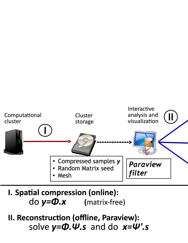
Figure 1: A schematic showing the major steps during the in-situ data compression using CS (I) and the offline reconstruction and visualization of the original dataset (II) using Paraview. The random seed, the mesh and the compressed samples $y$ are transferred to the visualization platform where the reconstruction of $x$ takes place.

We have implemented the reconstruction procedure in two ways: 1) in Matlab in order to experiment and produce some of the results shown below, and 2) a more production-oriented version written using the Trilinos sparse linear algebra library [18] and ParaView for visualization [19].

4 Results

In this section we discuss the compression capability and reconstruction quality of our method. We also describe some aspects of its practical implementation. We consider two types of data defined on unstructured meshes. The first type are “toy problems” where we assume mathematical functions defined on an irregular two-dimensional geometry. These datasets are small, and we can compress and reconstruct them on one processor. The second type are larger datasets obtained from simulations. In this case, we consider unstructured three-dimensional meshes distributed among many processors.

4.1 Two-dimensional datasets

We consider a square geometry with randomly chosen holes such that it constitutes an irregular geometry. We discretize it using a triangular mesh consisting of $N=33,067$ nodes. We assume two functions $f$ and $g$ given in Eqs. 11 and 12 as the datasets represented on the obtained mesh. We choose these functions such that $f$ exhibits multiple oscillations and reveals more features than $g$. The motivations behind this choice is that we would like to explore the effect of data features on the number of samples $y$ required during compressed sensing, that are necessary to accurately reconstruct the original dataset.

$$f =48\text{sin}(8\pi x)\text{sin}(7\pi y)\text{sin}(6\pi x)$$ (11)

$$g =12\text{sin}(2\pi x)\left[4\text{sin}(2\pi x)-4\text{sin}(2\pi y)\right]$$ (12)

We compress $f\in\mathbb{R}^{N}$ and $g\in\mathbb{R}^{N}$ using a random Bernoulli matrix $\Phi\in\mathbb{R}^{M\times N}$ as described in Section 2.1. We select an Alpert wavelet basis and reconstruct $f$ using the StOMP algorithm described in Section 2.3. Both compression and reconstruction are performed in a serial run. We denote the reconstructed fields by $f^{r}$ and $g^{r}$, respectively. They are plotted in Figure 2 which shows that the original and reconstructed datasets are visually identical. The function $f$ that reveals many features; a minimum compression ratio of $R=10$ was required for its accurate reconstruction. However, $g$ affords a higher compression ratio $R=30$ since it has fewer features which incur more data redundancy. This result indicates the possibility to predict the compression ratio in terms of the global gradient. This latter increases with the number of features in a given dataset. Such prediction of the compression ratio is extremely important in-situ since the compressibility of the datasets is unknown a priori.

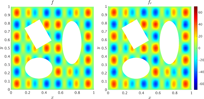
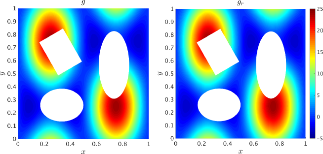
Figure 2: Plots showing (left column) smooth datasets represented on a complex geometry and an unstructured mesh of 33,067 nodes, and (right column) their reconstructed version from compressed samples, at full wavelet detail. The top and bottom rows denote two different datasets given by Eqs. 11 and 12, respectively. The compression ratios are $R=10$ and $R=30$ for $f$ and $g$, respectively. The bases for reconstruction are Alpert wavelets with an order $w=5$.

In order to obtain a quantitative description of the reconstruction accuracy, we evaluate the global $L_{2}$ norm of difference between the original and reconstructed versions. Figure 3 shows this error for $f$ and $g$ as a function of the wavelet order for different compression ratios. As expected, the error is lower for low compression ratios. We notice that there exists a minimum compression ratio required to obtain a low reconstruction error i.e. a correct reconstruction. For example, the compression ratio should be smaller than $30$ for the dataset $g$. This is consistent with the Donoho chart [17] which depicts a discontinuity in the compression ratio range that guarantees an accurate reconstruction.

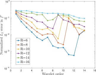
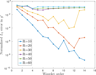
Figure 3: Plots showing the normalized $L_{2}$ error between the original and reconstructed datasets $f^{r}$ (left) and $g^{r}$ (right) plotted in Figure 2 as a function of the wavelet order for different compression ratios, as indicated.

The error decreases with the wavelets order $w$. The decreasing trend is reversed at larger values of $w$. This is mainly attributed to the over-fitting of the function $f$ by the high order Alpert polynomial wavelets. It is therefore preferred to choose lower orders. According to the plots in Figure 3, $w=5$ is an optimum value for the wavelet order that minimizes the reconstruction error and prevents over-fitting of the given function in the dataset.

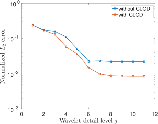
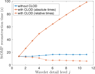
Figure 4: Plots showing (left) the normalized $L_{2}$ error and (right) the time taken in a serial run to perform the reconstruction of the dataset, as a function of the wavelet detail level $j$ for $w=5$. These results are reported using with and without the CLOD approach, as indicated.

The results presented so far are reported at the full wavelets detail level. We turn our attention now to the effect of the detail level on the reconstructed function quality. Such analysis is useful for datasets that exhibit multiple features. By construction, wavelets are able to represent all scales in a function where a scale $j$ reveals a level of detail as described in Section 2.2. In this work, we find the number of detail levels by performing orthogonal splits along each axis [13] which results in $j_{\text{max}}=11$ for $w=5$ for the mesh representing $f$. The wavelet matrix $\Psi$ is computed as the product of different detail level sparse matrices $\Psi_{j}$ [15, 16] following:

$$\Psi=\prod_{j=1}^{j=j_{\text{max}}}\Psi_{j}$$ (13)

$\Psi$ can be computed at any $1\leq j\leq j_{\text{max}}$ and used to perform a StOMP reconstruction. The sparsity of $\Psi$ decreases with $j$ to encode more details. Figure 5 shows the reconstructed function $f^{r}$ at different detail levels $j$. By scanning the figure, we notice how the fine details in the function are revealed. Changes between functions reconstructed at two consecutive detail levels decrease with $j$, indicating convergence. At $j=6$, the function is visually identical to the original $f$ in Figure 2.

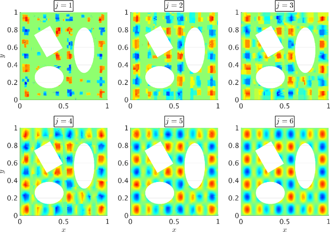
Figure 5: Plots showing the dataset in Figure 2 reconstructed at different wavelet detail levels $j$, as indicated. Results are generated from samples compressed with $R=10$ that are reconstructed with an Alpert wavelet basis of order $w=5$.

For each detail level, we consider two reconstruction approaches. In the first approach, the initial guess of the StOMP reconstruction is the same and assumes wavelet modes equal zero. In the second approach, an initial guess at a detail level $j$ is obtained from the solution at level $j-1$. Thus, we call this approach a continuous level of detail (CLOD) reconstruction. Figure 4 (left) shows the reconstruction error of the dataset $f$ as a function of the wavelet detail level. For both approaches, the error decreases with the detail level, as expected. However, the CLOD approach results in an error about three times lower at the finest details. This is due to the accumulation of knowledge in the reconstructed $f^{r}$ with consecutive detail levels. Figure 4 (right) shows the reconstruction time required at each level. Using CLOD, the relative time taken between two consecutive levels decreases with $j$ due to updated initial guess resulting in a decreased number of StOMP iterations. However, the cumulative time is substantially higher than the case without CLOD. The additional time required by CLOD to reach a smaller reconstruction error can be alleviated by skipping the reconstruction at some levels e.g. performing the CLOD reconstruction at the odd numbers levels.

4.2 Three-dimensional distributed datasets

In this section, we consider a larger dataset represented on a three-dimensional tetrahedral mesh with 396,264 points. The data is the temperature field obtained by a transient heat conduction simulation. The cylindrical geometry constitutes several sub-domains of different solid materials. The sub-domains sizes, heat conductivity and heat generations rates are chosen in a random fashion which results in a heterogeneous temperature distribution. Initially, the temperature is uniform across the domain, after which, it evolves to a steady state. The simulation is performed in parallel on 16 processors and the datasets is split equally among the processors ( 24,766 point per processor). The compression is performed locally on each processor i.e. the matrix-vector product in Eq. 1 was performed serially on each processor with no communications with other processors. Doing so preserves an efficient in-situ compression, and a faster and memory-efficient StOMP reconstruction on the visualization workstation. The whole dataset can be recovered by assembling the different reconstructed portions. Figure 6 shows the original and reconstructed versions of the steady state temperature fields for different portions of the dataset corresponding to different processors. For a compression ratio $R=10$, the reconstructed and original datasets are in a visual agreement.

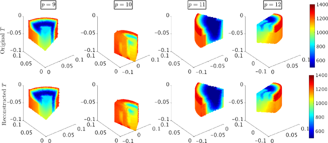
Figure 6: Plots showing the steady state temperature distributions in different portions of the three-dimensional (top) original and (bottom) reconstructed dataset $T$. Results are reported from a parallel simulation on 16 processors where compression is performed locally with a ratio $R=10$. The vertical panels correspond to almost equal portions of the full dataset as distributed among different processors, as indicated. The reconstruction is performed using StOMP for a wavelet order $w=5$ at full detail.

Finally, we report in Figure 7 (left) the evolution of the reconstruction error as a function of time for a constant compression ratio $R=$.10 The error is initially large since at earlier times, large gradients exist in the dataset. As heat diffuses in the domain, the temperature field becomes smoother and better represented by the wavelet bases. It leads to a smaller reconstruction error. Overall, the error decreases with larger wavelet orders as expected. We notice a saturation in the error and even a slightly increased error for higher orders mainly at early times. Similar to the test cases in Section 4.1, this is due by the over-fitting of the high gradients in the temperature field by the higher order Alpert wavelets. These results suggest that local large gradients form discontinuities and contribute to the overall reconstruction error. Therefore, when predicting the compression ratio in-situ, the local gradients have to be accounted for along the global gradient discussed in Section 4.1.

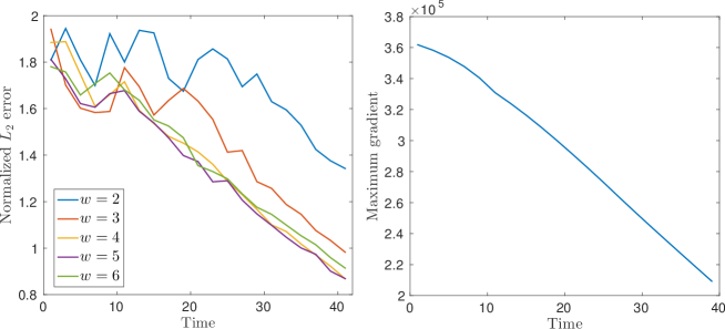
Figure 7: Plots showing the variation of the reconstruction error in the dataset $T$ as a function of time. Results are reported from a parallel simulation on 16 processors where compression is performed locally with a ratio $R=10$. The reconstruction is performed using StOMP at full detail for different wavelet orders $w$, as indicated.

5 Conclusion

In this paper we have demonstrated an application of compressive sensing to unstructured mesh data. We used second generation wavelets to efficiently represent the irregularities present in the spatial geometries and meshes. We are able to achieve lossy compression ratios of between 10 and 30 on fields defined on these meshes, depending on the oscillations and features present in the data. The visual deterioration as a result of the lossy compression at those rates is minimal. Large gradients and discontinuities in the data also contribute in assessing the reconstruction quality. We explored continuous level of detail reconstruction for datasets exhibiting many features and found that it results in a lower reconstruction error at the expense of an increased computational cost. We continue to explore ways to improve the algorithms used here in terms of reconstruction time and streaming. It may also be the case that other wavelet and sampling matrix pairs and reconstruction algorithms will produce better results on some data. We continue to investigate these as well.

6 Acknowledgements

The authors would like to acknowledge Dr. Jaideep Ray for providing valuable discussions and feedback that were helpful to accomplish this work.

This work was supported by the Laboratory Directed Research and Development (LDRD) program at Sandia National Laboratories.

Sandia National Laboratories is a multi-program laboratory managed and operated by Sandia Corporation, a wholly owned subsidiary of Lockheed Martin Corporation, for the U.S. Department of Energy’s National Nuclear Security Administration under contract DE-AC04-94AL85000.

- [1] S. Klasky, H. Abbasi, J. Logan, M. Parashar, K. Schwan, and A. Shoshani et al. In situ data processing for extreme scale computing. In Proceedings of SciDAC 2011, July 2011.
- [2] Sriram Lakshminarasimhan, Xiaocheng Zou, David A Boyuka Ii, Saurabh V Pendse, John Jenkins, Venkatram Vishwanath, Michael E Papka, Scott Klasky, and Nagiza F Samatova. DIRAQ: scalable in situ data-and resource-aware indexing for optimized query performance. Cluster Computing, 17(4):1101–1119, 2014.
- [3] Peter Lindstrom. Fixed-rate compressed floating-point arrays. Visualization and Computer Graphics, IEEE Transations on, 20(12):2674–2683, 2014.
- [4] H. Yu, C. Wang, R.W. Grout, J.H. Chen, and K. Ma. In situ visualization for large-scale combustion simulations. IEEE Computer Graphics and Applications, 30(3):45–57, 2010.
- [5] F. Sauer, H. Yu, and K. Ma. An analytical framework for particle and volume data of large-scale combustion simulations. In Proceedings of the 8th International Workshop on Ultrascale Visualization. ACM, New York, USA, 2013.
- [6] N. Fabian, K. Moreland, D. Thompson, A.C. Bauer, P. Marion, B. Geveci, M. Rasquin, and K.E. Jansen. The paraview coprocessing library: A scalable, general purpose in situ visualization library. In 2011 IEEE Symposium on Large Data Analysis and Visualization (LDAV), 2011.
- [7] J. Woodring, J. Ahrens, J. Figg, J. Wendelberger, S. Habib, and K. Heitmann. In situ sampling of a large scale particle simulation for interactive visualization and analysis. SIAM Journal on Mathematical Analysis, 30(3):1151–1160, 2011.
- [8] J.C. Bennett, S. Comandur, A. Pinar, and D. Thompson. Sublinear algorithms for in-situ and in-transit data analysis at the extreme-scale. In DOE Workshop on Applied Mathematics Research for Exascale Computing, Washington DC, USA, August 2013.
- [9] Emmanuel Candes and Michael Wakin. An introduction to compressive sampling. IEEE Signal Processing Magazine, 25(2):21 – 30, 2008.
- [10] Yaakov Tsaig and David Donoho. Extensions of compressed sensing. Signal Processing, 86(3):533–548, 2006.
- [11] A. Borghi, J. Darbon, S. Peyronnet, T.F. Chan, and S. Osher. A simple compressive sensing algorithm for parallel many-core architectures. Journal of Signal Processing Systems, 71:1–20, 2013.
- [12] M. Jansen and P. Oonincx. Second Generation Wavelets and Applications. Springer, 2005.
- [13] W. Sweldens. The lifting scheme: a construction of second generation wavelets. SIAM Journal on Mathematical Analysis, 29(2):511–546, 1998.
- [14] D.M. Radunovic. Wavelets from Math to Practice. Springer, 2009.
- [15] Bradley Alpert, Gregory Beylkin, Ronald Coifman, and Vladimir Rokhlin. Wavelet-like bases for the fast solution of second-kind integral equations. SIAM Journal on Scientific Computing, 14(1):159–184, 1993.
- [16] Bradley K Alpert. A class of bases in L2 for the sparse representation of integral operators. SIAM journal on Mathematical Analysis, 24(1):246–262, 1993.
- [17] D. L. Donoho, Y. Tsaig, I. Drori, and J-L Starck. Sparse solution of underdetermined systems of linear equations by stagewise orthogonal matching pursuit. IEEE Transactions on Information Theory, 58(2):1094–1121, 2012.
- [18] Michael A. Heroux, Roscoe A. Bartlett, Vicki E. Howle, Robert J. Hoekstra, Jonathan J. Hu, Tamara G. Kolda, Richard B. Lehoucq, Kevin R. Long, Roger P. Pawlowski, Eric T. Phipps, Andrew G. Salinger, Heidi K. Thornquist, Ray S. Tuminaro, James M. Willenbring, Alan Williams, and Kendall S. Stanley. An overview of the trilinos project. ACM Trans. Math. Softw., 31(3):397–423, 2005.
- [19] K. Moreland, D. Rogers, J. Greenfield, B. Geveci, P. Marion, A. Neundorf, and K. Eschenberg. Large scale visualization on the cray xt3 using paraview. In Cray User Group, May 2008.