Weak values are quantum: you can bet on it

Abstract

The outcome of a weak quantum measurement conditioned to a subsequent postselection (a “weak value” protocol) can assume peculiar values. These results cannot be explained in terms of conditional probabilistic outcomes of projective measurements. However, a classical model has been recently put forward that can reproduce peculiar expectation values, reminiscent of weak values. This led the authors of that work to claim that weak values have an entirely classical explanation. Here we discuss what is quantum about weak values with the help of a simple model based on basic quantum mechanics. We first demonstrate how a classical theory can indeed give rise to non-trivial conditional values, and explain what features of weak values are genuinely quantum. We finally use our model to outline some main issues under current research.

More than 25 years ago Aharonov, Albert, and Vaidman have introduced a measurement protocol whose outcome was termed Weak Value (WV). Aharonov1988 This protocol utilizes a weak measurement that avoids the collapse of the system’s wave function, conditioned on a specific outcome of a subsequent strong (projective) measurement –termed postselection. For a generic quantum mechanical system prepared in a state $|i\rangle$, if $A$ is the operator measured weakly, and $|f\rangle$— the system’s state corresponding to the successful postselection, the weak value obtained by the above procedure is $A_{w}=\langle f|A|i\rangle/\langle f|i\rangle$.

A major feature of such a conditional measurement protocol, which has attracted much attention, is that the weak value can be, by far, larger than the standard quantum expectation value of the measured observable. In a recent publication Ferrie and Combes have pointed out that such large values may also be obtained from a strictly classical protocol that involves conditional probabilities. Ferrie2014 As a result, they went on to argue that “there is nothing quantum in WVs”. Theirs is just the latest of a series of works that, over the years, have come up with classical analogues of the weak value protocol and associated paradoxes (see e.g., Ref. Kirkpatrick2003, ), followed by appropriate clarifications (see e.g. Refs. Dressel2012, ; Ravon2007, ). It appears that the question still lingers: is it indeed true that the main features of WVs can be reproduced following a purely classical protocol?

Well, not quite. The essential difference between classical and quantum protocols is inherent to the fact that classically one may acquire information on a system without disturbing it, while quantum mechanically, measurement necessarily leads to disturbance of the system. The implications on quantum WVs, as opposed to their classical counterparts, are quite striking. To have a strong influence of the post selection measurement on the initial one within a classical protocol, the latter needs to ”know” about the former. Strong perturbation of the first measurement on the system is needed. By contrast, large quantum WVs can be obtained for arbitrarily small disturbance of the system by the measurement apparatus. Another fundamental difference is that no probabilistic classical model can consistently reproduce all post-selected outcomes of a quantum system.

To demonstrate the point of view of Ferrie and Combes, we rephrase their simple and appealing example in the form of a parameter’s estimation problem. Note1 Consider a particle prepared in either of two boxes according to a probability distribution: $p_{1}$ is the probability to find it in box 1, and $p_{2}=1-p_{1}$ — the probability to be in box 2. The two boxes define our system. Having at our disposal a statistical ensemble of such systems, we are interested in determining (measuring) $p_{1}$ and $p_{2}$. This is achieved by the following protocol (cf. Fig. 1): in each repetition of the experiment the boxes are opened and, if the particle is in box 1 it will emit a signal with probability $P(S|1)=1/2+\lambda$; if instead the particle is in box 2, it emits a signal with probability $P(S|2)=1/2-\lambda$.

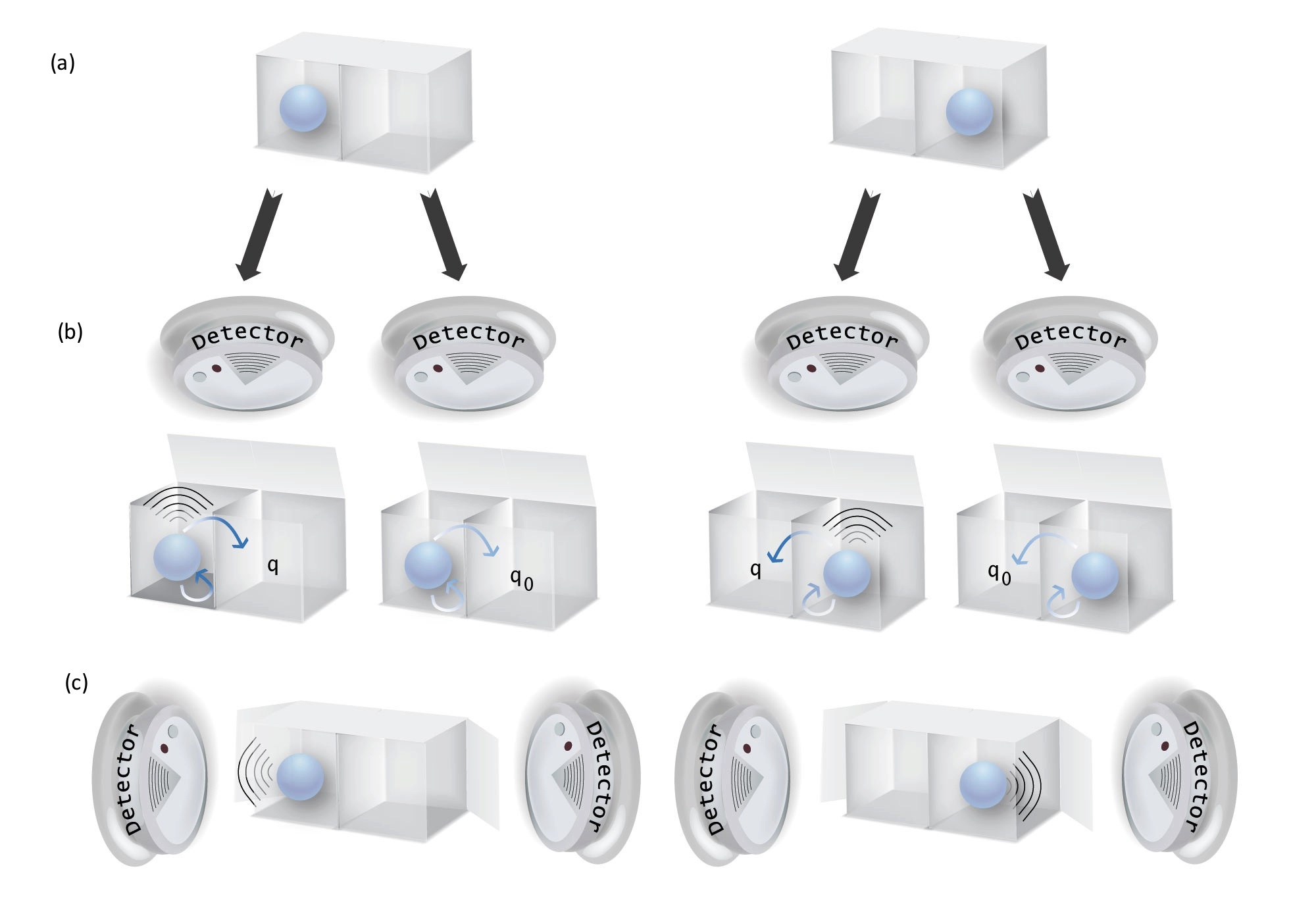
Figure 1: A classical protocol for estimation of the occupation probabilities of box 1 and 2. (a) Preparation. Possible initial states of the system —the system is prepared (with different probabilities) with either box 1 or box 2 occupied. (b) Measurement and disturbance. During the measurement a signal may be emitted (and then detected), with different probabilities, depending on which box the particle is in. The measurement is accompanied by a subsequent disturbance on the system; the particle changes its box location with probability $q$ or $q_{0}$, depending on whether a signal was emitted or not. (c) Post-selection. Following the measurement, the two possible final configurations (left or right) are unambiguously (strongly) detected.

The probabilities of not-emitting a signal are $P(\bar{S}|1)=1/2-\lambda$ and $P(\bar{S}|2)=1/2+\lambda$ respectively. Note that $\lambda$ is a parameter of the detection scheme, which is known a-priori. In fact, it controls how “good” our measurement is: for $\lambda\to 0$ we do not learn anything about the system and the measurement is weak; by contrast, $\lambda=1/2$ maximizes the information that can be extracted from the system — the measurement is strong. Since $p_{1}+p_{2}=1$, it is sufficient to estimate $p_{1}-p_{2}$. To do so we average the statistical data with properly assigned values of the outcome $S$, ( $\alpha_{S}=1/\lambda$) and $\bar{S}$, ($\alpha_{\bar{S}}=-1/\lambda$). The signal average is then

$$\langle S\rangle=\alpha_{S}P_{S}+\alpha_{\bar{S}}P_{\bar{S}},$$ (1)

where $P_{S}$ and $P_{\bar{S}}$ are the probabilities of detecting or not detecting a signal respectively, estimated simply as the number of detected events (or non-detected events), divided by the total number of trials. The values $\alpha_{S}$ and $\alpha_{\bar{S}}$ are, in fact, a special case of so-called contextual values; Dressel2010 they guarantee that $\langle S\rangle=p_{1}-p_{2}\in[-1,1]$, regardless of what the probabilities $p_{1}$, $p_{2}$ are. We now introduce disturbance and postselection by adding another step to this protocol: should a signal be emitted (upon opening the boxes), the particle has probability $q$ to switch its position between box 1 and box 2; should there be no signal emitted, switching of the particle between the two boxes will happen with probability $q_{0}$. We finally check the location of the particle. We define the conditional signal average: this is the average $\langle S\rangle$ , conditioned on the subsequent event f of finding the particle in box 2. It is equal to

$${}_{f}\langle S\rangle=\alpha_{S}P_{S|f}+\alpha_{\bar{S}}P_{\bar{S}|f}=\frac{1}{\lambda}\left(P_{S|f}-P_{\bar{S}|f}\right).$$ (2)

Operationally, the conditional probabilities are equal to the number of events of $S$ or $\bar{S}$, given the subsequent event $f$ (finding the particle in box 2), divided by all trials where $f$ is found. We define the classical analog of the weak value as

$$A_{w}^{(\textrm{classical})}=\lim_{\lambda\to\infty}{}_{f}\langle S\rangle.$$ (3)

If no disturbance is introduced, this conditioned average is bounded, $A_{w}^{(\textrm{classical})}\in[-1,1]$, with the same boundaries of the unconditioned signal.

This classical protocol should be compared to its quantum analog. In the latter, the state of the system is not described by a probability distribution, but rather by a density matrix. We assume for simplicity that the system is in a pure state, $\rho=|i\rangle\langle i|$, with $|i\rangle=\sqrt{p_{1}}|1\rangle+\sqrt{1-p_{1}}|2\rangle$. Our quantum detector, which is weakly coupled to the system (the two boxes) with strength $\lambda$, then measures the operator $A=|1\rangle\langle 1|-|2\rangle\langle 2|$. It extracts an ambiguous signal with two possible outcomes ($S$, $\bar{S}$), analogously to the classical case (see Ref. Ferrie2014, ). Consistently assigning contextual values ($\alpha_{S}$,$\alpha_{\bar{S}}$) to these outcomes, the average over the statistical data yields $\langle S\rangle=\alpha_{S}P_{S}+\alpha_{\bar{S}}P_{\bar{S}}=\langle i|A|i\rangle$. This is the same as the classical outcome. Now, following this measurement we consider a unitary evolution (let it be not the most general one), which transforms the states $|1\rangle$ and $|2\rangle$ to $|f\rangle$ and $|\bar{f}\rangle$, e.g., $|2\rangle\to|\bar{f}\rangle=\cos(\theta/2)|1\rangle+\sin(\theta/2)|2\rangle$, with $\theta\in[0,2\pi]$. The conditional average of the measurement’s outcome with a successful post-selection on box 2 is then given, in the limit of weak measurement, $\lambda\to 0$, by the weak value

$$A_{w}^{(\textrm{quantum})}=\lim_{\lambda\to 0}{}_{f}\langle S\rangle=\frac{\langle f|A|i\rangle}{\langle f|i\rangle}=\frac{\sqrt{p_{1}\sin(\frac{\theta}{2})}+\sqrt{(1-p_{1})\cos(\frac{\theta}{2})}}{\sqrt{p_{1}\sin(\frac{\theta}{2})}-\sqrt{(1-p_{1})\cos(\frac{\theta}{2})}}.$$ (4)

The weak value obtained for any pre- and post-selection in the quantum model can be reproduced by the conditional outcome of the classical model, i.e. $A_{w}^{(\textrm{quantum})}=A_{w}^{(\textrm{classical})}$, upon choosing specific initial state and parameters. This has led Ferrie and Combes to conclude that “weak values are not quantum”. The simple example used to put forward their claim Ferrie2014 employed $\sqrt{p_{1}}=\cos(\theta/2)$, hence $A_{w}^{(\textrm{quantum})}=1/\cos(\theta)$. The same large number is reproduced through the classical model in the weak coupling limit ( $\lambda\to 0$ ) by choosing $p_{1}=1$, $q_{0}=(\cos\theta-\lambda)/(1-\lambda)$, $q=(\cos\theta+\lambda)/(1+\lambda)$.

This example, following the footsteps of several others Kirkpatrick2003 ; Dressel2012 , unambiguously demonstrates that the mere fact that weak values can be arbitrarily large is not per se a unique feature of quantum mechanics. In what way is then the weak value a genuine quantum mechanical entity? First of all, no classical model can consistently reproduce the weak values of a quantum system and all post-selected states. In fact, as nicely highlighted in Ref. Dressel2015, ; Pusey2014, , were this the case in a classical protocol, along with large weak values, some post-selection events would have to occur with negative probabilities!!

A more quantitative way for discerning the quantum nature of weak values is to focus on the detector’s back-action on the system. In the quantum case, the weaker the measurement ($\lambda\to 0$), the lesser is the postselection probability modified from its unperturbed value; nonetheless, large weak values can emerge. This is to be contrasted with a classical protocol, also in the weak measurement limit. In order to obtain the same large value (now of $A_{w}^{(\textrm{classical})}$), one needs to modify the post-selection probability substantially. Dressel2015 ; Hoffmann2014 In the simple classical model outlined by Ferrie and Combes, the postselection probability in the absence of measurement is identically zero; when performing the weak measurement the change in the post selection probability is $P(f)=P(f|S)+P(f|\bar{S})\sim\cos\theta\gg\lambda$. The qualitative difference with the infinitesimal change of post-selection probability in the quantum case is evident, and may be put on a quantitative basis. Ipsen2015 One can look at the minimal back-action for fixed information acquired by the detector in the classical and quantum cases. Trivially, in the former it is possible to attain zero backaction; in the quantum case a finite minimal back-action is unavoidable. An important observation is that one obtains the Aharonov-Albert-Vaidman weak value as the weak measurement limit of a conditioned average in a wide class of models, where the detector minimally disturbs the system. Dressel2012 ; Ipsen2015 How to define weak values as minimal backaction limit over a wide family of quantum measurement protocols is the subject of current research.

It is clear from the above that, while anomalous classical conditional values imply a large disturbance, and they depend on the (arbitrarily chosen) value of the latter, quantum weak values conform to the minimum back-action requirement. In fact, postselected measurements with minimum back-action offer an operational approach to deal with conditional averages in the quantum realm. The related weak values have been used as a new tool to define physical quantities not amenable to simple, direct strong measurement (e.g., tunneling time, Steinberg1995 many-body cotunneling time Romito2014 ). In short, not only are weak values quantum, but they also constitute an interesting tool to explore hidden facets of quantum mechanics. Much of this remains a challenge for the future.

References

- (1) Y. Aharonov, D. Albert, L. Vaidmann, Phys Rev. Lett. 60 (1998).
- (2) C. Ferrie, J. Combes, Phys. Rev. Lett. 113 120404 (2014).
- (3) K. Kirkpatrick, J. Phys. A: Math. Gen. 36, 4891–900 (2003).
- (4) J. Dressel, A.N. Jordan, J. Phys. A: Math. Theor. 45 015304 (2012).
- (5) T. Ravon, L. Vaidman, J. Phys. A: Math. Theor. 40 2873 (2007).
- (6) Note that all the ingredient of the model in Ref. Ferrie2014 are present in previous models, see e.g. Refs. Kirkpatrick2003, ; Dressel2012, ; Ravon2007, .
- (7) J. Dressel, A. Agarwal, A. Jordan, Phys. Rev. Lett. 104, 240401 (2010).
- (8) J. Dressel, Phys. Rev. A 91, 032116 (2015).
- (9) M.F. Pusey, Phys. Rev. Lett. f113, 200401 (2014).
- (10) H. Hoffmann, M. Iinuma, Y. Shikano, arXiv:1410.7126 (2014).
- (11) A. Ipsen, Phys. Rev. A 91, 062120 (2015).
- (12) A. M. Steinberg, Phys. Rev. Lett. 74, 2405 (1995); Y. Choi, A.N. Jordan, Phys. Rev. A 88, 052128 (2013).
- (13) A. Romito, Y. Gefen, Phys. Rev. B 90, 085417 (2014).