Restricted Indian Buffet Processes

Abstract

Latent feature models are a powerful tool for modeling data with globally-shared features. Nonparametric exchangeable models such as the Indian Buffet Process offer modeling flexibility by letting the number of latent features be unbounded. However, current models impose implicit distributions over the number of latent features per data point, and these implicit distributions may not match our knowledge about the data. In this paper, we demonstrate how the Restricted Indian Buffet Process circumvents this restriction, allowing arbitrary distributions over the number of features in an observation. We discuss several alternative constructions of the model and use the insights gained to develop Markov Chain Monte Carlo and variational methods for simulation and posterior inference.

1 Introduction

Generative models are a popular approach for identifying latent structure in data. For example, a musical piece may be naturally modeled as a collection of notes, each with associated frequencies. A patient’s health may be naturally modeled as a collection of diseases, each with associated symptoms. The text of a news article may be naturally modeled as a collection of topics, each with associated words. In each of these cases, we posit that there exists a small set of underlying features that are responsible for generating the structure that we observe in the data.

When the number of these underlying features is unknown, Bayesian nonparametric models such as the Indian Buffet Process (IBP) Griffiths and Ghahramani, (2011) provide an elegant generative modeling approach. Specifically, the IBP posits that there are an infinite number of potential underlying features, but only a finite number of features underlie any particular observation. The IBP has been the foundation for a variety of modeling applications including choice behavior Görür et al., (2006), psychiatric comorbitities Ruiz et al., (2014), network models Miller et al., (2009), blind source separation Knowles and Ghahramani, (2007), image modeling Zhou et al., (2009), and time-series models Fox et al., (2009).

Under the IBP, the prior distribution over the number of features underlying an observation is governed by a single parameter $\alpha$. The number of features in an observation is expected a priori to be distributed as $\mbox{Poisson}(\alpha)$. The two-parameter Griffiths and Ghahramani, (2011) and three-parameter Teh and Görür, (2009) extensions of the IBP retain this strong requirement for Poisson-distributed feature cardinality. Other non-parametric latent variable models such as the infinite gamma-Poisson process Titsias, (2008) and the beta-negative Binomial process Broderick et al., (2015); Zhou et al., (2012) also exhibit a Poisson distribution over the number of non-zero features. Even IBP variants that posit various kinds of correlations between observations Gupta et al., (2013); Miller et al., (2008) or features  Doshi-Velez and Ghahramani, (2009) retain the Poisson property on the number of features in each observation. Caron, (2012) somewhat relaxes the Poisson constraint; their model allows the number of features underlying each observation to follow a mixture of Poissons.

However, there may be situations in which we do not desire Poisson-distributed marginals. For example, power law behaviors are common in networks and natural language. In medicine, the number of patients visiting a clinic without severe illnesses may be much more than predicted by a Poisson distribution. When modeling articles, we may wish to preclude the possibility of having no topics represented. Image data may come with labels, and the text of the label might provide strong clues about the number of objects we can expect to see in the image. In other settings, we may know exactly the number of active features associated with an observation. For example, when modeling audio recordings, the number of speakers in each recording might be known. The IBP does not provide the flexibility to put an arbitrary prior distribution on the number of latent features in an observation; even with the mixture of Poissons allowed by Caron, (2012) we are constrained to overdispersed distributions with full support on the non-negative integers.

In this article, we present and describe the Restricted Indian Buffet Process (R-IBP), a recently developed model that allows an arbitrary prior distribution to be placed over the number of features underlying each observation. Unlike the model of Caron, (2012), this distribution can have arbitrary support, or even be degenerate on a single value. The R-IBP was originally presented in Williamson et al., (2013); this paper extends upon that exposition. We present several alternative constructions, new insights, and novel efficient inference techniques.

2 Background: Completely random measures and Infinite Exchangeable Matrices

Many Bayesian nonparametric models, including the IBP, can be expressed in terms of completely random measures (CRMs) Kingman, (1967). A completely random measure $\mu$ is a random measure consisting of a collection of atoms $\mu=\sum_{i}\pi_{i}\delta_{\theta_{i}}$ on some space $(\Theta,\mathcal{A})$ such that for any disjoint subsets $A_{1},A_{2}\in\mathcal{A},A_{1}\cap A_{2}=\emptyset$, the masses $\mu(A_{1}),\mu(A_{2})$ assigned to those subsets are independent.

The atom sizes $\pi_{i}$ and locations $\theta_{i}$ and are governed by a Lévy measure $\nu(d\pi,d\theta)$; different choices of the Lévy measure yield different properties. For example, the Lévy measure $\nu(d\pi,d\theta)=c\alpha\pi^{-1}(1-\pi)^{\alpha-1}d\pi H(d\theta)$ describes the homogeneous beta process Hjort, (1990), whose name reflects the fact that the atom sizes $\pi_{i}$ are equal in distribution to the limit as $I\rightarrow\infty$ of $\mbox{Beta}\left(\frac{c\alpha}{I},c\left(1-\frac{\alpha}{I}\right)\right)$ random variables. The Lévy measure $\nu(d\pi,d\theta)=\gamma\pi^{-1}e^{-\lambda\pi}d\pi H(d\theta)$ describes the gamma process, whose atom sizes similarly correspond to the infinitesimal limit of a gamma distribution. We will write an arbitrary CRM with Lévy measure $\nu(d\pi,d\theta)$ as $\mbox{CRM}\left(\nu(d\pi,d\theta)\right)$.

CRMs can be used to construct distributions over matrices with exchangeable rows and infinitely many columns. To do so, we first define a directing measure $\mu:=\sum_{i=1}^{\infty}\pi_{i}\delta_{\theta_{i}}\sim\mbox{CRM}\left(\nu(d\pi,d\theta)\right)$ to be a CRM with Lévy measure $\nu$. We then let $\zeta_{n}:=\sum_{n=1}^{\infty}z_{ni}\delta_{\theta_{i}}\stackrel{{\scriptstyle\mbox{\tiny{i.i.d.}}}}{{\sim}}\mbox{CRM}(g(\mu)),n=1,2,\dots$ be a sequence of CRMs whose Lévy measure is some functional $g(\mu)$ of this directing measure $\mu$. Then, following de Finetti, the sequence $\zeta_{1},\zeta_{2},\dots$ is an infinitely exchangeable sequence of measures. If we consider only the atom sizes $z_{ni}$ of these measures, then we can transform this sequence of exchangeable measures into a sequence of exchangeable vectors $Z_{n}=(z_{n1},z_{n2},\dots)$. Stacking these (infinitely long) vectors results in a matrix $\mathbf{Z}=(Z_{1},\dots,Z_{n})$ with exchangeable rows.

One of the most commonly used models in this class is the beta-Bernoulli process Thibaux and Jordan, (2007), which defines a distribution over infinitely exchangeable binary matrices. The directing measure $\mu$ is distributed according to a beta process

$$\mbox{BP}(c,\alpha,H):=\mbox{CRM}\left(c\alpha\pi^{-1}(1-\pi)^{\alpha-1}d\pi H(d\theta)\right),$$

where $c,\alpha>0$ and $H$ is a probability measure on $\Theta$. Conditioned on $\mu$, the $\zeta_{n}$ are distributed according to a Bernoulli process

$$\mbox{BeP}(\mu):=\mbox{CRM}\left(\delta_{1}(d\pi)\mu(d\theta)\right).$$

The number of non-zero entries in each row of the resulting matrix will be finite, but random; marginally, this number will be distributed as $\mbox{Poisson}(\alpha)$.

Since the beta process and the Bernoulli process form a conjugate pair, we can integrate out the directing beta process measure and work directly with the exchangeable sequence of binary vectors. When $c=1$, the resulting exchangeable distribution is known as the Indian Buffet Process Griffiths and Ghahramani, (2011), and the predictive distribution can be described in terms of the following analogy: Let each column of our matrix correspond to a dish in an infinitely-long buffet, and each row correspond to a customer. The first customer selects a $\mbox{Poisson}(\alpha)$ number of dishes. When the $n$th customer arrives at the buffet, there are a finite number of previously sampled dishes and an infinite number of unsampled dishes. He selects a dish that has previously been sampled $m_{i}$ times with probability $m_{i}/n$, and selects a $\mbox{Poisson}(\alpha/n)$ number of new dishes. For general $c\neq 1$, the corresponding exchangeable process is known as the two-parameter IBP Griffiths and Ghahramani, (2011); Thibaux and Jordan, (2007); a related restaurant analogy is given in Griffiths and Ghahramani, (2011).

The Indian Buffet Process can be used as the basis for a latent feature model where both the number of latent features exhibited by a given data point, and the total number of latent features, are unknown. In this context, each row of the matrix corresponds to a data point, and each column corresponds to a latent feature; a non-zero entry indicates that a given data point exhibits a given feature.

Different choices of CRMs yield different properties in the resulting matrix. For example, the three-parameter Indian Buffet Process replaces the beta process directing measure with a stable-beta process; the resulting random matrix exhibits power-law behavior in the total number of features exhibited in $N$ rows Teh and Görür, (2009). If we combine a gamma process directing measure with a sequence of Poisson processes, we obtain the infinite gamma-Poisson process Titsias, (2008), a distribution over integer-valued matrices. Other exchangeable matrices constructed in this manner include the beta-negative binomial process Zhou et al., (2012); Broderick et al., (2015) and the gamma-exponential process Saeedi and Bouchard-Côté, (2011).

3 Exchangeable Binary Matrices with Arbitrary Marginals: The Restricted Indian Buffet Process

The class of exchangeable matrices described in Section 2 offers significant modeling flexibility. One property, however, cannot be avoided by judicious choice of CRM: the distribution over the number of non-zero entries per row is always marginally Poisson. This property is a direct consequence of the complete randomness of the underlying random measures $\mu$ and $\zeta_{n}$. To show this property, we observe that, regardless of choice of directing measure, there will be some probability $\pi_{i}$ that the column $i$ is non-zero. Each column $i$ is chosen independently, resulting in a binomial distribution over the number non-zeros entries per row. With infinite columns, the binomial distribution converges to a Poisson distribution.

We can also show, intuitively, how imposing an arbitrary distribution over the number of non-zero entries must break the complete randomness. Suppose that we know that each row of our matrix has exactly $J$ non-zero entries. Next, suppose that we observe $J$ non-zero entries in the first $k$ columns. We know that the remaining (infinite) entries must be zero with probability one; the probabilities of the entries in the disjoint sets of columns $1\dots k$ and $(k+1)\dots$ are no longer independent. Complete randomness has been broken.

The Restricted Indian Buffet Process (R-IBP), first introduced in Williamson et al., (2013), is a distribution over exchangeable binary matrices with an arbitrary distribution over the number of non-zero entries per row. In the following sections, we describe several equivalent formulations for the R-IBP. While the focus is on restricted versions of the Indian Buffet Process, the ideas in this section can be similarly applied to build other matrices with arbitrary marginals, as we will describe in Section 4.

3.1 Construction of the R-IBP via Restriction in the de Finetti Representation

The R-IBP was originally constructed (in Williamson et al., (2013)) by manipulating the beta-Bernoulli process representation of the IBP. Recall from Section 2 that we can represent the IBP as a mixture of Bernoulli processes, directed by a beta process:

$$\begin{split}\mu:=\sum_{i}\pi_{i}\delta_{\theta_{i}}\sim&\mbox{BP}(c,\alpha,H)\\ \zeta_{n}:=\sum_{i}z_{ni}\delta_{\theta_{i}}\stackrel{{\scriptstyle\mbox{\tiny{i.i.d.}}}}{{\sim}}&\mbox{BeP}(\mu)\\ Z_{n}:=&(z_{ni})_{i=1}^{\infty}.\end{split}$$ (1)

Since we are not interested in the locations $\theta_{i}$ of the atoms, we will employ a slight misuse of notation and write Equation 1 as:

$$\begin{split}\mu\sim&\mbox{BP}(c,\alpha,H)\\ Z_{n}\stackrel{{\scriptstyle\mbox{\tiny{i.i.d.}}}}{{\sim}}&\mbox{BeP}(\mu).\end{split}$$ (2)

We can modify this construction to give a restricted model where the number of non-zero entries per row is constrained to be some integer $J$, by replacing the Bernoulli process in Equation 2 with a restricted Bernoulli process

$$\mbox{R-BeP}(Z_{n};\mu,f=\delta_{J})\propto\begin{cases}\mbox{BeP}(Z_{n};\mu)&\mbox{if }\sum_{i}z_{ni}=J\\ 0&\mbox{otherwise.}\end{cases}$$ (3)

where the associated normalizing constant is proportional to the probability that a random sample from a Bernoulli process has total mass $J$. More concretely, this gives

$$\begin{split}&\mbox{R-BeP}\left(Z_{n};\mu,f=\delta_{J}\right)\\ =&\frac{\prod_{i=1}^{\infty}\pi_{i}^{z_{ni}}(1-\pi_{i})^{1-z_{ni}}\mathbb{I}(\sum_{i}z_{ni}=J)}{\sum_{z^{\prime}\in\mathcal{Z}}\prod_{i}\pi_{i}^{z^{\prime}_{i}}(1-\pi_{i})^{1-z^{\prime}_{i}}\mathbb{I}(\sum_{i}z^{\prime}_{i}=J)},\end{split}$$ (4)

where $\mathcal{Z}$ is the support of $\mbox{BeP}(\mu)$.

This restricted Bernoulli process is the random measure obtained by conditioning the Bernoulli process on its total sum; it can be seen as a nonparametric extension of the conditional Bernoulli distribution Chen, (2000). Clearly it is no longer a completely random measure: disjoint subsets of $Z_{n}$ depend on each other via the total sum.

More generally, we may wish to have some arbitrary distribution $f$ on the number of non-zero entries per row. We can obtain this by creating an $f$-mixture of the distributions described by Equation 4, so that the probability of a vector $Z$ is given by

$$\mbox{R-BeP}(Z;\mu,f)\stackrel{{\scriptstyle d}}{{=}}f\left(\sum_{i}Z_{i}\right)\mbox{R-BeP}\left(Z;\mu,\delta_{\sum_{i}Z_{i}}\right).$$ (5)

We can substitute these restricted Bernoulli processes (Equations 4, 5) for the Bernoulli processes in Equation 2, yielding the following Restricted Indian Buffet Process:

$$\begin{split}\mu\sim&\mbox{BP}(c,\alpha,H)\\ Z_{n}\stackrel{{\scriptstyle i.i.d.}}{{\sim}}&\mbox{R-BeP}(\mu,f).\end{split}$$ (6)

Since the $Z_{n}$ are identically and independently distributed given $\mu$, de Finetti’s theorem tells us the resulting matrix $\mathbf{Z}=(Z_{n})_{n=1}^{N}$ has exchangeable rows.

We note that even if we choose $f(z)=\mbox{Poisson}(z;\alpha)$, we do not recover the IBP. The IBP has $\mbox{Poisson}(\alpha)$ marginals over the number of non-zero elements in each row; however, conditioned on observing some elements in a row, the number of non-zero entries in the remaining elements are distributed according to a Poisson-binomial distribution. Complete randomness requires that distribution over the non-zero elements in some subset of columns does not depend on the number of non-zero elements in a disjoint subset of columns. In contrast, an R-IBP with $f(z)=\mbox{Poisson}(z;\alpha)$ will retain $\mbox{Poisson}(\alpha)$ as the conditional distribution over the total number of non-zero entries, even after some entries have been observed.

3.2 Construction via Subsets of an Exchangeable Sequence

In Section 3.1, we saw how the R-IBP can be represented using the combination of a beta process directing measure and a sequence of restricted Bernoulli processes parametrized by this measure. Sometimes it is more convenient to work solely in terms of the exchangeable matrix $\mathbf{Z}$ (which has a finite number of non-zero columns), integrating out the (infinite-dimensional) directing measure $\mu$. We can make use of the IBP predictive distribution to represent the R-IBP without representing the underlying beta process; however care must be taken to ensure the correct distribution.

We can generate an IBP-distributed sequence $\mathbf{Z}^{*}=(Z^{*}_{1},Z^{*}_{2},\dots)$ of vectors using the buffet-based predictive distribution described in Section 2. Since this sequence is infinitely exchangeable, its law is invariant to shuffling the order of any finite subset Aldous, (1983). A direct consequence of this is that any infinite sub-sequence $\mathbf{Z}$ of $\mathbf{Z}^{*}$ is again infinitely exchangeable. Thus, we can construct an $\mbox{R-IBP}(c,\alpha,f)$-distributed matrix $\mathbf{Z}$ by sampling a sequence of vectors $\mathbf{Z}^{*}\sim\mbox{IBP}(c,\alpha)$, and including each proposed vector $Z_{n}^{*}$ into our matrix $\mathbf{Z}$ with probability $f(\sum_{i}Z^{*}_{ni})$.

We note that this is directly equivalent to the restricted Bernoulli process method described in Section 3.1: if we integrate out the directing measure, a sequence of Bernoulli process-distributed measures is described by the IBP. However, an undesirable property of the IBP-based procedure is that, unlike the Bernoulli process-based procedure, one must retain the entire sequence $\mathbf{Z}^{*}$ (or at least, its sufficient statistics) to generate the next candidate for $\mathbf{Z}$. If we generate our proposed distributions based on the column counts of $\mathbf{Z}$ rather than $\mathbf{Z}^{*}$, the resulting matrix will not have the desired law - and in general will not even be exchangeable.

To demonstrate this lack of exchangeability, we will attempt to construct a $\mbox{R-IBP}(c=1,\alpha,f=\delta_{1})$ matrix $\mathbf{Z}$ by generating candidate vectors for $Z_{n}$ based only on the counts of $Z_{1:n-1}$. As shown by Fortini et al., (2000) and Aldous, (1983), a sequence is infinitely exchangeable iff

$$(Z_{N+1},Z_{N+2})|(Z_{1},\dots,Z_{N})\stackrel{{\scriptstyle d}}{{=}}(Z_{N+2},Z_{N+1})|(Z_{1}\dots Z_{N}).$$

It therefore suffices to check whether $(Z_{2},Z_{3})|Z_{1}\stackrel{{\scriptstyle d}}{{=}}(Z_{3},Z_{2})|Z_{1}$. Let $P$ be the law of the IBP with parameters $1,\alpha$, and let $P^{*}$ be the law of the proposed variant. Since our restricting function $f=\delta_{1}$, trivially we have $P^{*}(Z_{1}=(1,0,0,\dots))=1$. We will compare $P^{*}(Z_{2}=(1,0,0,\dots),Z_{3}=(0,1,0,\dots))$ and $P^{*}(Z_{2}=(0,1,0,\dots),Z_{3}=(1,0,0,\dots))$.

Under the Indian Buffet Process, we have $P(Z_{2}=(1,0,0,\dots)|Z_{1}=(1,0,0,\dots))=\frac{1}{2}e^{-\alpha/2}$ and $P(Z_{2}=(0,1,0,\dots)|Z_{1}=(1,0,0,\dots))=\frac{\alpha}{4}e^{-\alpha/2}$; therefore if we restrict $Z_{2}$ to these two cases, $P^{*}(Z_{2}=(1,0,0,\dots))=\frac{2}{2+\alpha}$ and $P^{*}(Z_{2}=(0,1,0,\dots))=\frac{\alpha}{2+\alpha}$.

Following a similar argument,

$$\begin{split}&P^{*}(Z_{3}=(0,1,0,\dots)|Z_{1}=(1,0,0,\dots),Z_{2}=(1,0,0,\dots))\\ &=\frac{\alpha}{\alpha+6}\end{split}$$

and

$$\begin{split}&P^{*}((Z_{3}=(1,0,0,\dots)|Z_{1}=(1,0,0,\dots),Z_{2}=(0,1,0,\dots))\\ &=\frac{3}{6+2\alpha}.\end{split}$$

So,

$$\begin{split}&P^{*}(Z_{2}=(1,0,0,\dots),Z_{3}=(0,1,0,\dots))\\ &=\frac{2}{2+\alpha}\frac{\alpha}{\alpha+6}=\frac{2\alpha}{\alpha^{2}+8\alpha+12}\end{split}$$

and

$$\begin{split}&P^{*}(Z_{2}=(0,1,0,\dots),Z_{3}=(1,0,0,\dots))\\ &=\frac{\alpha}{2+\alpha}\frac{3}{6+2\alpha}=\frac{3\alpha}{2\alpha^{2}+10\alpha+12}.\end{split}$$

Clearly, $(Z_{2},Z_{3})|Z_{1}\stackrel{{\scriptstyle d}}{{\neq}}(Z_{3},Z_{2})|Z_{1}$ under the proposed construction, meaning the resulting sequence is not exchangeable. In order to construct an exchangeable sequence via the IBP, we must record the entire IBP-generated sequence and then select an appropriate sub-sequence.

3.3 Construction via Tilting the Bernoulli Process

A tilted CRM $\mu^{*}$ is a random measure obtained by scaling the law $P_{\mu}$ of a CRM $\mu$ on $(\Omega,\mathcal{A})$ by its total mass, according to some function $h(\Omega)$ Lau, (2013), so that

$$P_{\mu^{*}}(A):=\frac{1}{\mathbb{E}[h(\mu(\Omega))]}\int_{A}h(\nu(\Omega))P_{\mu}(d\nu).$$ (7)

For example, if $h(x)=e^{-\gamma x}$, then $\mu^{*}$ is said to be exponentially tilted. Exponentially tilting a CRM yields a different CRM Lau, (2013); for example an exponentially tilted $\alpha$-stable process is equal (in distribution) to a generalized gamma process Brix, (1999). In general, however, a tilted CRM will not be a completely random measure. For example, if $h(x)=x^{-q}$ for some $q>0$, then $\mu^{*}$ is said to be polynomially tilted and is no longer a CRM. Random measures constructed via polynomial tilting include the Pitman-Yor process Pitman and Yor, (1997) (obtained by polynomially tilting an $\alpha$-stable process) and the beta-gamma process James, (2005) (obtained by polynomially tilting a gamma process).

In Equation 5, the probability of a vector $Z_{n}$ under the restricted Bernoulli process is given by its probability under the Bernoulli process, scaled by a function $f$ of the number of nonzero entries in $Z_{n}$ (or equivalently, the total mass of the corresponding random measure $\zeta_{n}=\sum_{i}z_{ni}\delta_{\theta_{i}}$). Thus the restricted Bernoulli process can be described as a tilted Bernoulli process with the tilting function $h(x)=f(x)$.

3.4 Construction via the Normalized Beta Prime Process and Invariance with respect to the Directing Measure

As shown in Equation 2, the IBP can be written as a sequence of Bernoulli processes with a beta process directing measure $\mu$. If only a finite number $N$ of rows $Z_{n}$ have been observed, our uncertainty about $\mu$ is described by a beta process with parameters $c+N,\frac{c\alpha}{c+N}H+\frac{1}{c+N}\sum_{n=1}^{N}\zeta_{n}$. As $N$ tends to infinity, this posterior will tend towards the uniquely defined directing measure $\mu$.

In contrast, the beta process directing measure $\mu$ for the R-IBP can never be uniquely determined, even with infinitely many observations. To show this, we can re-construct the R-IBP in terms of a beta-prime process Broderick et al., (2014). A beta-prime process-distributed CRM $\tau:=\sum_{i}w_{i}\delta_{\theta_{i}}$ is obtained by transforming the atoms $\pi_{i}$ of a beta process-distributed CRM $\mu:=\sum_{i}\pi_{i}\delta_{\theta_{i}}$ according to

$$w_{i}:=\frac{\pi_{i}}{1-\pi_{i}}.$$

The de Finetti representation of the R-IBP can now be written as

$$\begin{split}\tau:=\sum_{i}w_{i}\delta_{\theta_{i}}\sim&\mbox{Beta-prime}(c,\alpha,H)\\ J_{n}\sim&f\\ P(Z_{n}|\tau,f)=&\frac{\prod_{i}w_{i}^{z_{i}}\mathbb{I}(\sum_{i}z_{ni}=J)}{\sum_{z^{\prime}\in\mathcal{Z}}\prod_{i}w_{i}^{z^{\prime}_{i}}\mathbb{I}(\sum_{i}z_{ni}=J)}.\end{split}$$ (8)

The law $P(Z_{n}|\tau,f)$ is invariant to rescaling the $w_{i}$ by some constant $e^{\beta}$, that is,

$$\mbox{R-BeP}(Z;\{w_{i}\},J)\stackrel{{\scriptstyle d}}{{=}}\mbox{R-BeP}(Z;\{e^{\beta}w_{i}\},J)$$

for any $\beta\in\mathbb{R}$. Rescaling the beta-prime process weights $w_{i}$ by $e^{\beta}$ is equivalent to rescaling the atoms $\pi_{i}$ of the corresponding beta process according to the nonlinear function

$$\pi_{i}^{\prime}=\frac{\pi_{i}e^{\beta}}{\pi_{i}e^{\beta}+1-\pi_{i}},$$ (9)

which describes the Esscher transform of a Bernoulli random variable Gerber and Shiu, (1993). Intuitively, this scale invariance occurs because the R-IBP first chooses the number of non-zero entries $J_{n}\sim f$ and then selects which entries will be non-zeros. Conditioned on $J_{n}$, the absolute scale of the weights $\pi$ no longer matters; only their relative sizes are important.

The connection between the restricted IBP and the beta-prime process makes it possible to remove extra degree of freedom present in the beta-Bernoulli (or beta-prime-Bernoulli) construction by fixing the scale through a normalized beta-prime process. While this is theoretically appealing – it leads to a unique directing measure for each infinite sequence – it offers little practical advantage, due to the lack of a tractable representation for such a process.

4 Extensions and Variations

In Section 3, we focused on exchangeable models based on the IBP. However, the same ideas apply to exchangeable models based on other completely random measures. One can also relax the exchangeability assumption to allow partial exchangeability, leading to models appropriate for data with observation-specific covariates.

4.1 Restricted Exchangeable Matrices based on Different Completely Random Measures

In Section 3.1 we showed that the Restricted IBP can be constructed by starting from the beta-Bernoulli process representation of the IBP, and replacing the Bernoulli process with a restricted Bernoulli process. Rather than start from the beta-Bernoulli process, we could pick any pair of CRMs to generate an exchangeable sequence $(\zeta_{n})_{n=1}^{N}$, provided we can parametrize the $\zeta_{n}$ using the directing measure $\mu$, for example if $\mu$ and $\zeta_{n}$ form a conjugate pair Orbanz, (2009):

$$\begin{split}\mu\sim&\mbox{CRM}\left(\nu(d\pi,d\theta)\right)\\ \zeta_{n}\stackrel{{\scriptstyle\mbox{\tiny{i.i.d.}}}}{{\sim}}&\mbox{CRM}(g(\mu)),n=1,2,\dots\end{split}$$ (10)

If the support of the random measures $\zeta_{n}$ in Equation 10 consists almost surely of measures with a finite number of non-zero atoms, the resulting exchangeable sequence can be interpreted as a row-exchangeable matrix with a finite number of non-zero columns. Examples of such exchangeable matrices include the beta-negative binomial process Zhou et al., (2012); Broderick et al., (2015) and the gamma-Poisson process Titsias, (2008). All such models exhibit the property that the total number of non-zero elements of a row are (marginally) Poisson-distributed, a direct consequence of the complete randomness of the underlying random measures (as described in Section 3).

For any such exchangeable model, we can restrict the support of the $\zeta_{n}$ to generate an exchangeable matrix with restricted support. If $\zeta_{n}\sim\mbox{BeP}(\mu)$, this amounts to placing some distribution $f$ over the number of non-zero entries, as described in Section 3.1. For other choices of CRM, however, the support of the unrestricted measure will not be limited to binary vectors, presenting a wider range of possible restrictions. We discuss three possibilities below.

Restricting the number of non-zero entries per row

If $\zeta_{n}$ is distributed according to a Bernoulli process, imposing a distribution over the sum of a row is equivalent to imposing a distribution over the number of non-zero entries. For more general CRMs, these two cases are not the same. We first consider imposing a function $f\left(\sum_{k}\mathbb{I}(z_{k}>0)\right)$ on the number of non-zero entries. This yields a restricted CRM with law

$$\begin{split}&\mbox{R-CRM}^{(1)}\left(Z;g(\mu),f\left(\sum_{k}\mathbb{I}(z_{k}>0)\right)\right)\\ \propto&f\left(\sum_{k}\mathbb{I}(z_{k}>0)\right)\mbox{CRM}(Z;g(\mu))\end{split}$$ (11)

where $CRM(g(\mu))$ is the law of the corresponding unrestricted CRM.

Restricting the sum of each row

We can also impose a function $f(\sum_{k}z_{k})$ on the total sum of each row (or equivalently the total mass of each measure $\zeta_{n}$), yielding

$$\begin{split}&\mbox{R-CRM}^{(2)}\left(Z;g(\mu),f\left(\sum_{k}z_{k}\right)\right)\\ \propto&f\left(\sum_{k}z_{k})\right)\mbox{CRM}(Z;g(\mu))\end{split}$$ (12)

A special case of the construction in Equation 12 is obtained when the directing measure $\mu$ is distributed according to a gamma process with parameter $\alpha H$ for some probability measure $H$, and the $\zeta_{n}$ are distributed according to a Poisson process with mean measure $\mu$ Titsias, (2008). In this case, if we restrict the total sum of each row following Equation 12, the distribution over the $\zeta_{n}$ is equivalent to that given by the following Dirichlet process-multinomial model:

$$\begin{split}\rho\sim&\mbox{DP}(\alpha,H)\\ J_{n}\sim&f\\ \zeta_{n}\sim&\mbox{Mult}(\rho,J_{n})\end{split}$$

Restricting the sum of each row and the value of each element

The examples in Equations 11 and 12 give a taste of the sort of distributions available under this construction. We can also specify more complex restrictions. For example, we could generate an exchangeable binary matrix with $J$ non-zero elements by taking letting the $\zeta_{n}$ be a CRM with integer-valued atoms, and restricting both the number of non-zero elements to be $J$ and the values of the non-zero elements to be one. If the directing measure $\mu$ is distributed according to a gamma process, and the $\zeta_{n}$ are distributed according to a Poisson process, each row corresponds to sampling $J$ entries using conditional Poisson sampling from a Dirichlet-distributed random measure.

4.2 Restricted Partially-Exchangeable Matrices

In Section 3, we assumed that our data points (or equivalently, the rows of our matrix) are exchangeable. We can however modify the R-IBP to yield a partially exchangeable model appropriate for data with observation-specific covariates. For example, each observation might have an associated label indicating a group membership $m\in\{1,\dots,M\}$, and each group could have group-specific restricting distribution $f_{m}$, so that

$$\begin{split}\mu\sim&\mbox{BP}(c,\alpha,H)\\ Z_{n}\stackrel{{\scriptstyle i.i.d.}}{{\sim}}&\mbox{R-BeP}(\mu,f_{m(n)}).\end{split}$$

where $m(n)$ is covariate describing the group for observation $n$. The resulting matrix would be partially exchangeable in the sense that the distribution is invariant to permuting rows belonging to the same group.

This model would be appropriate where we have observation-specific information about the number of non-zero features. For example, we might wish to construct a topic model with different distributions over the number of topics depending on the type of document (novels contain many topics, news articles contain fewer topics). Or, we might have a feature extraction task with labeling information indicating the expected number of features per observation – for example, in image modeling we might have descriptions or low-level labeling.

5 Simulation from the R-IBP

In Section 3, we presented several constructions for the R-IBP. These constructions result in a variety of approaches for sampling from the R-IBP prior. In this section, we discuss exact and approximate approaches for sampling from the R-IBP.

5.1 Sub-sampling from an Exchangeable Model

In Section 3.2, we showed that the R-IBP can be constructed by subset selection of an IBP-distributed sequence of binary vectors. This directly suggests a scheme for generating exact from the prior. We generate a sequence $\mathbf{Z}^{*}=(Z_{n}^{*})$ according to the Indian Buffet Process predictive distribution:

$$\begin{split}m_{ni}=&\sum_{j=1}^{n-1}z_{nj}^{*}\\ K^{+}_{n}=&\sum_{k}\mathbb{I}(m_{ni}>0)\\ z_{ni}^{*}\sim&\mbox{Bernoulli}(m_{ni}/n)\mbox{ for }i=1,\dots,K^{+}_{n}\\ \lambda_{n}\sim&\mbox{Poisson}(\alpha/n)\\ z_{nj}^{*}=&1\mbox{ for }j=K_{n}^{+}+1,\dots,K_{n}^{+}+\lambda\end{split}$$

Then, we include each $Z_{n}^{*}=(z_{n1}^{*},z_{n2}^{*},\dots)$ in our sequence $\mathbf{Z}$ with probability $P(Z_{n}^{*}\in\mathbf{Z})=f(\sum_{i}z_{ni}^{*})$. Importantly, while not all the generated binary vectors $Z_{n}^{*}$ are included in $\mathbf{Z}$, they are all included in the counts $m_{ni}$, ensuring exchangeability is maintained. Rejection sampling in an exchangeable model produces perfect samples from the R-IBP, but can suffer from a low acceptance rate.

5.2 Approximate Sampling with a Conditionally Independent Model

An alternative approach, inspired by the construction in Section 3.1, is to explicitly sample the directing measure $\mu\sim\mbox{BP}(c,\alpha,H)$ (or, alternatively, sample $\tau\sim\mbox{Beta-prime}(c,\alpha,H)$), and use this to sample a sequence $\mathbf{Z}^{*}=(Z_{n}^{*})$ of binary vectors. Practically speaking, we cannot represent the entire infinite-dimensional measure $\mu$ (or $\tau$). However, we can work with finite-dimensional approximations to $\mu$ to produce both approximate and exact samples. We describe approximate approaches in this section and an exact approach in section 5.3.

We first need to produce a finite set of weights $\pi$ that well approximate the infinite-dimensional measure $\mu$. We consider two options:

• Weak Limit One approach is to use a finite vector of beta random variables that converges (in a weak limit sense) to the beta process Zhou et al., (2009), approximating $\mu$ with a vector $\tilde{\pi}=(\tilde{\pi}_{1},\dots,\tilde{\pi}_{I})$, where

  $$\tilde{\pi}_{i}\stackrel{{\scriptstyle\tiny{iid}}}{{\sim}}\mbox{Beta}\left(\frac{c\alpha}{I},c-\frac{c\alpha}{I}\right).$$ (13)

• Size-Ordered Stick-breaking Representation Another approach is to transform the arrival times of a unit-rate Poisson process based on the beta process Lévy measure Rosiński, (2001); Ferguson and Klass, (1972). This approach gives exact samples from the size-ordered atoms of the beta process. In the special case where $c=1$, this yields a simple stick-breaking construction Teh et al., (2007):

  $$\begin{split}u_{i}\sim&\mbox{Beta}(\alpha,1)\\ \pi_{i}=&\prod_{j=1}^{i}u_{i}.\end{split}$$ (14)

  If we let our truncated approximation $\tilde{\pi_{i}}=\pi_{i}$ for $i=1\dots I$ and $\tilde{\pi_{i}}=0$ for $i>I$, we obtain an approximation to a sample from a beta process.

Given an approximate sample $\tilde{\pi}=(\tilde{\pi}_{1},\dots,\tilde{\pi}_{I})$ from our directing measure, there are a number of methods to simulate $Z_{n}\sim\mbox{BeP}(\tilde{\pi})$. We discuss several approaches below.

5.2.1 Rejection Sampling

Using a Bernoulli Process Proposal

Conditioned on $\tilde{\pi}$, it is straightforward to sample binary vectors $Z^{*}$ according to a Bernoulli process, by sampling $z^{*}_{i}\sim\mbox{Bernoulli}(\pi_{i}),i=1,\dots,I$. We can use these binary vectors as proposals in a rejection sampler. If $f$ is the desired distribution over the number of non-zero entries per row, we accept a proposal $Z^{*}$ with probability $f(\sum_{i}z^{*}_{i})$. Because we have explicitly instantiated (an approximation to) the directing measure $\mu$, the rows of $Z$ are i.i.d. and we do not need to maintain the sufficient statistics of the rejected binary vectors.

Using a tilted Bernoulli process proposal

The rejection sampling procedure using a Bernoulli process proposal will give low acceptance rates—and therefore high computational cost—if the target distribution $f$ differs significantly from the $\mbox{Poisson}(\alpha)$ distribution implied by the IBP. We can improve the acceptance rate—and hence ameliorate the computational costs—by exponentially tilting the Bernoulli process likelihood, as described in Section 3.4.

If we tilt a Bernoulli process (or, equivalently, scale the beta process-distributed directing measure according to Equation 9 and use the scaled directing measure as the base measure for a Bernoulli process), we change the distribution over the number of non-negative entries Brostrom and Nilsson, (2000). If we restrict the tilted Bernoulli process, however, the distribution is not affected by the tilting parameter $\beta$, i.e.

$$\begin{split}&\mbox{R-BeP}((\tilde{\pi}_{1},\dots,\tilde{\pi}_{I}))\\ \stackrel{{\scriptstyle d}}{{=}}\,&\mbox{R-BeP}\left(\left(\frac{e^{\beta}\tilde{\pi}_{1},}{e^{\beta}\tilde{\pi}_{1}+1-\tilde{\pi}_{1}}\dots,\frac{e^{\beta}\tilde{\pi}_{1},}{e^{\beta}\tilde{\pi}_{I}+1-\tilde{\pi}_{I}}\right)\right).\end{split}$$

We can maximize the likelihood of getting exactly $J$ non-negative entries, by setting $\beta$ to be the unique solution to

$$J=\sum_{i=1}^{I}\frac{e^{\beta}\tilde{\pi}_{i}}{e^{\beta}\tilde{\pi}_{i}+1-\tilde{\pi}_{i}}\,.$$

Thus, we can first sample the number of features $J_{n}$ on the $n$th row from $f$, Esscher transform the weights $\tilde{\pi}_{i}$ to maximize the chance of getting exactly $J_{n}$ non-zero entries, and then sample $Z_{n}$ using the transformed weights. For computational efficiency, the transformed weights can be cached for each value of $J_{n}$.

Discussion of approximation quality

As $I\rightarrow\infty$, both the weak-limit approximation of Equation 13 and the stick-breaking construction of Equation 14 will give exact samples from the R-IBP. However, a finite $I$ will introduce errors. When a stick-breaking representation for $\mu$ is used, then we know that all weights $\pi_{j}$, $j>I$ will be less than $\pi_{I}$. In particular, the iterative nature of the stick-breaking construction means that, if we exclude the first $I$ atoms $\pi_{1},\dots,\pi_{I}$, and scale the remaining atoms by $\pi_{I}$, we are left with a (strictly ordered) sample from the beta process.

We can consider the error introduced by this construction by considering the values of $z_{nj}$ that are excluded due to the truncation. If there are any non-zero elements $z_{nj}$ for $j>I$, our rejection probability will not be correct. Since the weights $\pi_{j},j>I$ are described by a scaled beta process, we know that the number of excluded non-zero elements will be distributed as $\mbox{Poisson}(\alpha\pi_{I})$. So, with probability $1-\mbox{Poisson}(0;\alpha\pi_{I})=1-\exp(-\pi_{I}\alpha)$ the true sum $\sum_{i}^{\infty}z_{ni}\neq\sum_{i}^{I}z_{ni}$ and thus we may incorrectly reject or accept a proposal..

We will reject incorrectly if there are any non-zero elements $z_{nj}$ for $j>I$. If we let $\mu=\sum_{i=1}^{\infty}\pi_{i}\delta_{\theta_{i}}$, where the $\pi_{i}$ are strictly size-ordered, and sample $Z_{n}^{*}$ from the Bernoulli process $\mbox{BeP}(\mu)$, it follows that the distribution over the number of non-zero elements for $z_{nj},j>I$ is given by $\sum_{i=I}^{\infty}z_{ni}^{*}\sim\mbox{Poisson}(\alpha\pi_{I})$. The probability that all elements are zero is given by $P(\sum_{i=I}^{\infty}z_{ni}^{*}=0)=\exp(-\pi_{I}\alpha)$. Thus, with probability $1-\exp(-\pi_{I}\alpha)$, the true sum $\sum_{i}^{\infty}z_{ni}\neq\sum_{i}^{I}z_{ni}$ and thus we may reject incorrectly.

Specifically, in the case where $f=\delta_{J}$, three possible outcomes exist when we propose a binary vector $Z^{*}$ from a size-ordered truncated approximation $\mbox{BeP}((\pi_{i},\dots,\pi_{I}))$:

1. $\sum_{i=1}^{I}z_{i}^{*}>J$: We reject the proposal. This is always correct.

2. $\sum_{i=1}^{I}z_{i}^{*}=J$: We accept the proposal. However, if the truncated tail has $\sum_{i=I+1}^{\infty}z_{i}^{*}>0$, we should really have rejected. Our decision is correct with probability $P(\sum_{i=I+1}^{\infty}z_{i}^{*}=0)=\exp(-\pi_{I}\alpha)$.

3. $\sum_{i=1}^{I}z_{i}^{*}<J$: We reject the proposal. However, if $\sum_{i=1}^{I}z^{*}_{i}=J-k$ but the truncated tail has $\sum_{i=I+1}^{\infty}z_{i}^{*}=k$, we will really should have accepted. Our decision is correct with probability $1-P(\sum_{i=I+1}^{\infty}z_{i}^{*}=J-\sum_{i=1}^{I}z_{i}^{*})=1-\mbox{Poisson}(J-\sum_{i=1}^{I}z^{*}_{i};\pi_{I}\alpha)$.

We will use this enumeration to construct an exact sampler in section 5.3.

5.2.2 Sampling using Inclusion Probabilities

Even with tilting, rejection sampling can be computationally expensive if $f$ differs significantly from $\mbox{Poisson}(\alpha)$. Given a finite-dimensional approximation to $\tilde{\pi}$ to the directing measure, an alternative is to use a draw-by-draw procedure based on computing the inclusion probabilities $P(z_{ni}|\tilde{\pi},k_{n})$ of each feature Aires, (1999). The marginal inclusion probability $\eta_{k;J}$ that feature $k$ is included in a sample of size $J$ is given by

$$\eta_{k;J}=\tilde{\pi}_{k}\frac{S_{J-1}^{I-1}(\tilde{\pi}_{1},...,\tilde{\pi}_{k-1},\tilde{\pi}_{k+1},...,\tilde{\pi}_{I})}{S_{J}^{I}(\tilde{\pi}_{1},...,\tilde{\pi}_{I})}$$ (15)

where $S_{J}^{I}$ corresponds to the probability of sampling $J$ elements from the set of $I$ features if each feature was chosen independently with probability $\tilde{\pi}_{i}$:

$$\textstyle S_{J}^{I}=\sum_{s\in A_{J}(I)}\prod_{k\in s}\tilde{\pi}_{k}\prod_{j\ni s}(1-\tilde{\pi}_{j})$$ (16)

where $A_{J}(I)$ is the set of all samples of size $J$ that can be drawn from the elements $I$. Fortunately, there is a recursion for calculating the values $S_{J}^{I}$ can be computed in $O(I^{2})$-time:

$$S_{J}^{I}=\tilde{\pi}_{I}S_{J-1}^{I-1}(\tilde{\pi}_{1},...,\tilde{\pi}_{I-1})+(1-\tilde{\pi}_{I})S_{J}^{I-1}(\tilde{\pi}_{1},...,\tilde{\pi}_{I-1})$$ (17)

and thus with appropriate caching, all of the elements $\eta_{k,J}$ can be computed (and cached) in $O(I^{3})$ time, and any Esscher transform (Equation 9) of the $\tilde{\pi}_{k}$ can be used in the recursions above.

Given the marginal inclusion probabilities $\eta_{ik}$, we now have a draw-by-draw algorithm for sampling a row $Z_{n}$ from the prior:

1. Sample the total number of features $J_{n}\sim f$.

2. Set $J=J_{n}$.

3. For each feature $k\in\{1,\dots,I\}$:

   1. Sample $z_{nk}\sim\mbox{Bernoulli}(\eta_{k,J})$.

   2. If $z_{nk}=1$, then decrement $J\leftarrow J-1$.

Discussion of approximation quality

If a size-ordered stick-breaking representation is used to approximate the weights $\pi$, then we can directly bound the errors on the inclusion probabilities as functions of the truncation level $I$, the size of the smallest instantiated weight $\pi_{I}$, and the function $f$. To do so, we first expand the expression for the probabilities $S^{\infty}_{J}$, starting with equation 16:

$$\textstyle S_{J}^{\infty} = \sum_{s\in A_{J}(I)}\prod_{k\in s}\pi_{k}\prod_{j\ni s}(1-\pi_{j})$$

$$+\sum_{s\ni A_{J}(I)}\prod_{k\in s}\pi_{k}\prod_{j\ni s}(1-\pi_{j})$$

$$= \exp(-\pi_{I}\alpha)\sum_{s\in A_{J}(I)}\prod_{k\in s}\pi_{k}\prod_{j\ni s,j\leq I}(1-\pi_{j})$$

$$+\sum_{s\ni A_{J}(I)}\prod_{k\in s}\pi_{k}\prod_{j\ni s}(1-\pi_{j})$$

$$= \exp(-\pi_{I}\alpha)S^{I}_{J}+\sum_{s\ni A_{J}(I)}\prod_{k\in s}\pi_{k}\prod_{j\ni s}(1-\pi_{j})$$

where $A_{J}(I)$ are still the sets in which all $J$ non-zero entries occur in the first $I$ columns. The second line follows because the probability of that all the columns $j>I$ are zero is $\exp(-\pi_{I}\alpha)$.

Since the probability of at least on non-zero element in columns $j>I$ is $1-\exp(-\pi_{I}\alpha)$, the second term is bounded between $0$ and $1-\exp(-\pi_{I}\alpha)$. Thus we can bound the inclusion probabilities

$$\eta_{k;J}=\pi_{k}\frac{S_{J-1}^{\infty}(\pi_{1},...,\pi_{k-1},\pi_{k+1},...,\pi_{I})}{S_{J}^{\infty}(\pi_{1},...,\pi_{I})}$$

$$\geq \pi_{k}\frac{e^{-\pi_{I}\alpha}S_{J-1}^{I-1}(\pi_{1},...,\pi_{k-1},\pi_{k+1},...,\pi_{I})}{e^{-\pi_{I}\alpha}S_{J}^{I}(\pi_{1},...,\pi_{I})+(1-e^{-\pi_{I}\alpha})}$$

$$\leq \pi_{k}\frac{e^{-\pi_{I}\alpha}S_{J-1}^{I-1}(\pi_{1},...,\pi_{k-1},\pi_{k+1},...,\pi_{I})+(1-e^{-\pi_{I}\alpha})}{e^{-\pi_{I}\alpha}S_{J}^{I}(\pi_{1},...,\pi_{I})}$$

As expected, the quality of the approximation depends not only truncation $I$ (and associated $\pi_{I}$) but also on the values $S^{I}_{J}$. If the probability of sampling $J$ elements from the first $I$ is low, then the approximation will be poor because it is likely that additional columns would have been required to sample $J$ elements.

5.3 Exact Sampling in a Conditionally Independent Model

We consider rejection sampling in an R-IBP with restricting function $f=\delta_{J}$, where we accept or reject proposals $Z^{*}\sim\mbox{BeP}((\pi_{i},\dots,\pi_{I}))$. In Section 5.2.1, working with a truncated version of $\mu$ obtained using a stick-breaking representation means that some proposals are erroneously rejected or accepted, due to the absence or presence of non-zero elements below the truncation. In particular, there were two cases in which we could make mistakes: if $\sum_{i}^{I}Z^{*}_{ni}<J$, we might reject incorrectly; if $\sum_{i}^{I}Z^{*}_{ni}=J$, we might accept incorrectly. To circumvent the uncertainty in these outcomes, we use a dynamic truncation to obtain exact samples from the R-IBP by using retrospective sampling Papaspiliopoulos and Roberts, (2008).

• Sample an initial truncated directing measure $\pi_{1}\dots\pi_{I}$ according to the size-ordered stick breaking representation of the Beta process (Equation 14).

• For $n=1,\dots,N$, repeat the following proposal step until we have accepted a row $Z_{n}$:

  • Sample $z^{*}_{1}\dots z^{*}_{I}\sim\pi_{1}\dots\pi_{I}$, and compute the sum $K^{*}=\sum_{i=1}^{I}z^{*}_{i}$.

    • If $K^{*}>J$, reject $Z^{*}$.

    • If $K^{*}=J$, accept with probability $\exp(-\pi_{I}\alpha)$.

    • If $K^{*}<J$,

      • Reject with probability $1-\mbox{Poisson}(J-\sum_{i}z_{ni};\pi_{I}\alpha)$.

      • Otherwise, expand the representation by sampling new $\pi_{i},z^{*}_{i}$ for $i=I+1,I+2,\dots$ according to the stick breaking representation, until $\sum z^{*}_{n}=J$. Accept the resulting $Z^{*}$, and update $I$ and $\pi$ to incorporate the new atoms.

We can adapt this procedure to arbitrary restricting function $f$, by first sampling a row count $J_{n}\sim f$ for each row. The growth of the truncation level $I$ will depend on $f$; if $J_{n}\sim f$ is large then we may have to expand to very large truncation levels $I$. Specifically, starting with a truncation level too small may result in many, many rejections before the truncation level is sufficiently expanded. However, the samples that we do accept will be from the correct R-IBP prior.

5.4 Empirical Comparison of Simulation Methods

We empirically compared the simulation approaches from Sections 5.1, 5.2.1, 5.2.2, and 5.3 by measuring the number of rejections and CPU time required to generate samples from the R-IBP with concentration parameter $\alpha=5$ and restricting function $f=\delta_{J}$ for $J=\{2,5,8\}$. We generated 25 samples of 100 observations from each of the five approaches: exact collapsed rejection sampling (Section 5.1), approximate uncollapsed rejection sampling and tilted approximate uncollapsed rejection sampling (Section 5.2.1), approximate inclusion sampling (Section 5.2.2), and exact uncollapsed rejection sampling (Section 5.3).

Rejections per 100 observations are shown in figure 1. As expected, rejection rates are lowest for $J=5$ because $\alpha=5$. Inclusion sampling, a draw-by-draw procedure, has no rejections, and tilting significantly reduces the number of rejections—and the variance in the number of rejections—regardless of $J$. The other procedures all have large rejection rates varying over several orders of magnitude. Figure 2 shows CPU time on a standard laptop. Again, the time to 100 acceptances is shortest when $J$ is equal to the expected value of features $\alpha$. The approximate methods are faster than the exact methods, and the approximate tilted rejection sampler is the fastest, closely followed by the approximate sampler that uses inclusion probabilities.

Figure 1: Rejections per 100 Acceptances

Figure 2: Time required for 100 Acceptances on a standard laptop

Figures 3 and 4 show the mean of the empirical feature probabilities, sorted in descending order, for various truncation levels for $J=5$ and $J=8$. When $J=5$, the exact samplers instantiate between 30-40 hidden features. The mean probabilities of the approximate methods follow the exact probabilities relatively closely even with truncations of $I=10$ or $I=20$, with only slight over-estimation to account for the fewer features. When $J=8$, the exact methods tend to instantiate 35-45 features. The approximate methods have a noticeable over-estimation of feature probabilities when the truncation $I$ is too small (e.g. $I=10$). However, as the truncation is increased, the mean probabilities from the approximate methods again closely match those from the exact methods. Interestingly, there do not seem to be large differences between the different approximate methods. These explorations suggest that the approximate methods can be accurate, computationally-efficient alternatives when the truncation is set to a reasonable value.

Figure 3: Mean of empirical feature probabilities, sorted in descending order for varying truncation levels and $J=5$

.

Figure 4: Mean of empirical feature probabilities, sorted in descending order for varying truncation levels and $J=8$

.

6 Posterior Inference in the R-IBP

In this section, we present approaches for posterior inference in the R-IBP. In Section 6.1, we present MCMC-based approaches related to the simulation techniques described in Section 5, and in Section 6.2 we present a computationally faster hybrid variational/MCMC approach for posterior inference.

6.1 MCMC-based Posterior Inference in the R-IBP

6.1.1 Collapsed Inference using an Augmented Representation

In Section 3.2, we showed that the R-IBP can be constructed by selecting subsets of an IBP, and in Section 5.1 we showed that this construction can be used to generate samples from the R-IBP prior. We can also use this construction to construct a collapsed Gibbs sampler, by reintroducing the discarded rows as auxiliary variables. For each data point $x_{n}$, let $Z_{n}$ be the associated latent R-IBP-distributed binary representation, let $t_{n}$ be an auxiliary variable indicating the number of discarded rows between observations $n-1$ and $n$, and let $c_{n}$ be an aligned auxiliary vector of counts associated with these discarded rows. Let $m_{i}=\sum_{n=1}^{N}(z_{ni}+c_{ni})$ be the total observed and auxiliary counts for the $i$th feature.

Sampling $t_{n}$ and $c_{n}$

When selecting a subset of the IBP, $t_{n}$ is the number of discarded samples between the $n-1$st and the $n$th accepted samples, and $c_{n}$ is the associated column counts. We can sample these directly, by sampling vectors $Z^{*}$ from the prior predictive distribution of the IBP given the remaining counts, $m+c_{-n}$. With probability $1-f(Z^{*})$, we include $Z^{*}$ in the auxiliary counts $c_{n}$ and $t_{n}$, and sample another vector; with probability $f(Z^{*})$ we do not include $Z^{*}$ in $c_{n}$ and stop our sampling procedure.

Sampling $Z_{n}$

We have two options for sampling $Z_{n}$. We can propose an entirely new vector $Z^{\prime}$, by using the ultimate $Z^{*}$ obtained when sampling $c_{n}$ (i.e. the proposal $Z^{*}$ that we rejected from $c_{n}$) as a Metropolis Hastings proposal. Since the proposal is sampled from the prior predictive distribution of the R-IBP, we accept the proposal with probability

$$\min\left(1,\frac{P(x_{n}|Z^{\prime}_{n},\Theta)}{P(x_{n}|Z_{n},\Theta)}\right)$$

Alternatively, we can propose smaller changes to the current vector $Z_{n}$. For example, we could propose $z^{\prime}_{ni}=1-z_{ni}$, and accept with probability $\min(1,r)$ where

$$\begin{split}r=&\frac{P(x_{n}|z_{ni}^{\prime},\mathbf{Z}_{-i},\Theta)P(z_{ni}^{\prime}|m_{-z_{ni}},N,\sum_{n}t_{n})}{P(x_{n}|z_{ni},\mathbf{Z}_{-i},\Theta)P(z_{ni}|m_{-z_{ni}},N,\sum_{n}t_{n})}\frac{q(z_{ni}^{\prime}\rightarrow z_{ni})}{q(z_{ni}\rightarrow z_{ni}^{\prime})}\\ =&\frac{P(x_{n}|z_{ni}^{\prime},\mathbf{Z}_{-i},\Theta)m_{i,-z_{ni}}^{z^{\prime}_{ni}}(1-m_{i,-z_{ni}}^{1-z^{\prime}_{ni}}f(z^{\prime}_{ni}+\sum_{k\neq i}z_{nk})}{P(x_{n}|z_{ni},\mathbf{Z}_{-i},\Theta)m_{i,-z_{ni}}^{z_{ni}}(1-m_{i,-z_{ni}}^{1-z_{ni}}f(z_{ni}+\sum_{k\neq i}z_{nk})}\end{split}$$

Similarly, we could propose changing multiple entries at once (necessary if we have, for example, $f(x)=\delta_{J}(x)$), or adding/removing new features.

6.1.2 Uncollapsed Inference with an Instantiated Latent Measure

If the distribution $f$ over the number of latent features per row differs significantly from that implied by the IBP, the number of auxiliary features required in a collapsed scheme quickly becomes prohibitive. In practice, we found the computational cost of the sampler described in Section 6.1.1 was infeasible in most cases.

An alternative approach is to alternate sampling the latent measure conditioned on the binary matrix, and vice versa, mirroring the methods for sampling from the prior described in Sections 5.2.1 and 5.2.2. Since we cannot represent the entire measure $\mu$, we work with a finite-dimensional approximation $\tilde{\pi}=(\tilde{\pi}_{1},\dots,\tilde{\pi}_{I})$, obtained either via a weak limit approximation or via truncation in a stick-breaking process. Sections 5.2.2 and 5.3 suggest methods for bounding the resulting error, or using a dynamic truncation to avoid such error.

Sampling $\mathbf{Z}|\tilde{\pi}$

If the distribution $f$ is not degenerate on a single point, we can use the inclusion probabilities described in Section 5.2.2, combined with $f$ and the data likelihood $P(X|Z,\Theta)$, to Gibbs sample the value of a single entry, using the conditional probabilities

$$\begin{split}&P(z_{ni}=1|\{\tilde{\pi}_{1},\dots,\tilde{\pi}_{I}\},\mathbf{Z}_{-ni},X,\Theta)\\ &\propto\tilde{\pi}_{i}\frac{S_{0}^{I-k_{n,-i}-1}(\{\tilde{\pi}_{k}:z_{nk}=0,k\neq i\})}{S_{1}^{I-k_{n,-i}}(\{\tilde{\pi}_{k}:z_{nk}=0\mbox{ or }k=i\})}\\ &\phantom{\propto}\cdot f(k_{n,-i}+1)P(X|z_{ni}=1,\mathbf{Z}_{-ni},\Theta)\\[5.0pt] &P(z_{ni}=0|\{\tilde{\pi}_{1},\dots,\tilde{\pi}_{I}\},\mathbf{Z}_{-ni},X,\Theta)\\ &\propto f(k_{n,-i})P(X|z_{ni}=0,\mathbf{Z}_{-ni},\Theta),\end{split}$$ (18)

where $k_{n,-k}=\sum_{j\neq k}z_{nj}$.

If the distribution $f$ is degenerate on a single value $J$, we cannot construct a Gibbs sampler that sequentially turns elements on or off; doing so would change the number of features. Instead, we can use the appropriate inclusion probabilities to sample the location of each of the non-zero elements in a row, conditioned on the other $J-1$ locations. Let $\ell_{nk}$ be the location of the $j$th non-zero entry. Then

$$\begin{split}&P(\ell_{nj}=i|\{\tilde{\pi}_{1},\dots,\tilde{\pi}_{I}\},\ell_{-nj},X,\Theta)\\ &\propto\tilde{\pi}_{i}\frac{S_{0}^{I-k_{n,-i}-1}(\{\tilde{\pi}_{k}:z_{nk}=0,k\neq i\})}{S_{1}^{I-k_{n,-i}}(\{\tilde{\pi}_{k}:z_{nk}=0\mbox{ or }k=i\})}\\ &\phantom{\propto}\cdot f(k_{n,-i}+1)P(X|\ell_{nj}=i,\ell_{-nj},\Theta)\end{split}$$ (19)

The Gibbs sampling steps described in Equations 18 and 19 only change a single element of $\mathbf{Z}$ at a time. This can lead to slow mixing. We can augment these Gibbs sampling steps with Metropolis Hastings proposals generated from the prior, using either the rejection sampling approach of Section 5.2.1 or the inclusion probability approach of Section 5.2.2 to propose an entire row of the binary matrix.

Sampling the latent measure

Once we have sampled our binary matrix $\mathbf{Z}$, we must resample our latent feature weights $\tilde{\pi}$. Unfortunately, since the beta process is not conjugate to the restricted Bernoulli process, we cannot directly Gibbs sample $\tilde{\pi}$ given $\mathbf{Z}$. Instead, we use Metropolis-Hastings steps. Since the posterior distribution over $\tilde{\pi}$ given $\mathbf{Z}$ is likely to be similar to the poster distribution in the unrestricted IBP, we use the posterior distribution from the unrestricted IBP as a proposal distribution. The acceptance probability depends on the R-IBP likelihood (Equations 4 and 5).

6.2 Hybrid Variational Inference in the R-IBP

The standard variational approach for the IBP Doshi et al., (2009) uses a mean-field approximation which places independent distributions $q(z_{ni})$ over each feature assignment $z_{ni}$. Using such a factored distribution is straightforward because each assignment $z_{ni}$ is drawn independently given the weight $\pi_{i}$. However, variational inference in the R-IBP is challenging because fixing the number of active features $J_{n}$ introduces dependence between the $z_{ni}$, and because the implied prior distributions over the marginal inclusion probabilities $\eta_{ik}$ are complex. Further, the invariance of the likelihood to scaling the directing measure, as described in Section 3.4, can lead to inefficiencies in exploring the state space and computational difficulties due to very small atom sizes that may occur at certain scales.

We propose a hybrid variational for inference in the R-IBP that combines variational distributions over the feature assignments and model parameters with MCMC inference over the directing measure. As in Section 6.1.2, we work with a finite dimensional approximation $\tilde{\pi}$ to the directing measure. We assume that the weights $\tilde{\pi}_{i}$ are fixed during the variational update, and then alternate between resampling the $\tilde{\pi}_{i}$ and updating the variational posterior on the other variables. We demonstrate this approach using a linear-Gaussian likelihood, where the data $X$ are assumed to be generated by $ZA+\epsilon$, where $A$ is an $I\times D$ feature matrix with independent normal priors $\mbox{Normal}(0,\sigma_{A}^{2})$ on each value and $\epsilon$ is a $N\times D$ matrix of independent noise drawn from $\mbox{Normal}(0,\sigma_{n}^{2})$. We note that the inference of the feature matrix $A$ is the same as in the standard IBP, and other likelihood models developed for the IBP can be substituted.

Specifically, the variables in the variational update are the feature assignments $Z$, the feature values $A$, and the count of active features per observation $J_{n}$. We consider the following mean field approximation for the variational inference:

• $q_{\phi_{i}}(A_{i})$ independent Gaussian distributions with mean $\phi_{i}$, variance $\Phi_{i}$ on the posterior of the feature value vector $A_{i}$.

• $q_{\nu_{ni}}(z_{ni})$ independent Bernoulli distributions, where $\nu_{ni}$ is the probability that $z_{ni}$ is active.

• $q_{\gamma_{nk}}(J_{n})$ multinomial distributions over the number of features in observation $n$, where $\gamma_{nk}$ is the probability that observation $n$ has $k$ active features.

Let ${W=\{\phi,\Phi,\nu,\gamma\}}$ be the set of variational parameters, and let ${V=\{A,Z,J_{n}\}}$ be the set of variables. Because the actual and variational distributions belong to the exponential family, coordinate ascent on the variational parameters corresponds to setting the variational distribution ${\log(q_{W_{i}})=E_{W_{-i}}[\log(P(W,V|X,\Theta))]}$, where $\Theta$ denotes the set of hyper-parameters $\{\sigma_{n}^{2},\sigma_{a}^{2},\alpha,f\}$ Wainwright and Jordan, (2008).

We focus on providing the variational updates for the parameters associated with $Z$ and $J_{n}$, as the updates for the parameters associated with $A$ (i.e., $\phi_{k},\Phi_{k}$) are exactly the same as in Doshi et al., (2009). The update for $\gamma_{nk}$ is:

$$\begin{split}\log(q_{\gamma_{n}}(J_{n}))=&E_{Z}[\log P(J_{n})+\log P(Z_{n}|\tilde{\pi},J_{n})]\\ =&\textstyle\sum_{k=1}^{K}I(J_{n}=k)[\log(f_{nk})+\nu_{ni}\log(\eta_{ik})\\ &+(1-\nu_{ni})\log(1-\eta_{ik})]\end{split}$$

where $f_{nk}$ is the prior probability that observation $n$ has $k$ elements. Exponentiating and normalizing, we recover the posterior parameters $\gamma_{nk}$.

The update for variational parameters $\nu_{ni}$ for the assignments $Z$ are also straightforward given the inclusion probabilities $\eta_{ik}$:

$$\begin{split}\log(q_{\nu_{ni}}(z_{ni}))=&E_{J_{n},Z_{-ni},A}[\log(P(z_{ni}|Z_{-ni},\tilde{\pi},J_{n}))\\ &+\log(P(X_{n}|Z_{n},A,\sigma_{n}^{2}))]\end{split}$$ (20)

where the second term is again exactly the same as in Doshi et al., (2009). For the first term, we can write

$$\begin{split}&E_{J_{n},Z_{-ni}}[\log(P(z_{ni}|Z_{-ni},\tilde{\pi},J_{n}))]\\ =&E_{J_{n},Z_{-ni}}[z_{ni}I(J_{n}=k)\log(\eta_{ik})\\ &\qquad+(1-z_{ni})I(J_{n}=k)\log(1-\eta_{ik})]\\ =&\textstyle z_{ni}\sum_{k}\gamma_{nk}\log(\frac{\eta_{ik}}{1-\eta_{ik}})+c\,.\end{split}$$ (21)

Substituting equation 21 into equation 20, we derive the update

$$\begin{split}\textstyle\xi=&\textstyle\sum_{k}\gamma_{nk}\log(\frac{\eta_{ik}}{1-\eta_{ik}})-\frac{1}{2\sigma_{n}^{2}}\bigg{(}-2\phi_{i}X_{n}^{T}+Tr(\Phi_{i})\\ &+\phi_{i}\phi_{i}^{T}+2\phi_{i}(\sum_{j\neq i}\nu_{nj}\phi_{j}^{T})\bigg{)}\\ \nu_{ni}=&\textstyle\frac{1}{1+\exp(-\xi)}\,.\end{split}$$ (22)

The equations above show how to update the variational distributions on $Z$, $A$, and $J_{n}$ given $\tilde{\pi}$. During our inference process, we iterate through the following steps:

1. Computing the partial variational posterior on $Z$, $A$, and $J_{n}$.

2. Sampling values of $Z$, $A$, and $J_{n}$ from the variational posterior.

3. Sampling new values of $\tilde{\pi}$ given the sampled $Z$.

To resample $\tilde{\pi}$ given $Z$, we use the Metropolis-Hastings step described in Section 6.1.2, where we jointly propose a new set of $\{\tilde{\pi}_{1}^{\prime}...\tilde{\pi}_{I}^{\prime}\}$ from the weak-limit approximation to the IBP posterior distribution ${\tilde{\pi}_{i}^{\prime}\sim\mbox{Beta}(\frac{\alpha}{I}+m_{i},1+N-m_{i})}$, where ${m_{i}=\sum_{n}z_{ni}}$. Next we accept or reject using the beta process prior on $\tilde{\pi}$ and the likelihood $P(Z|\tilde{\pi}^{\prime},J_{n})$, which can be computed using the inclusion probabilities $\eta^{\prime}_{ik}$.

7 Evaluation

We show a variety of evaluations to demonstrate the value of using the R-IBP on real and synthetic data when we have some knowledge about the marginals on the number of non-zero entries.

7.1 Exploration with Synthetic Data

To explore the ability of the R-IBP to recover latent structure, we generated two datasets using a linear Gaussian model, and used the IBP, the R-IBP with an appropriate restricting distribution, and the partially-exchangeable R-IBP with labeling information described in Section 4.2 to recover the latent structure.

7.1.1 Knowledge about the Number of Latent Features Assists with Parameter Recovery.

One reason for using the R-IBP is when we have strong ideas of what a “feature” corresponds to, coupled with strong information about the number of such features. While an IBP may be able to model the data using a collection of features, these features may not correspond to our preconceived notions of features – for example, the IBP might use multiple features where we expect a single feature.

To explore this, we generated a toy dataset with a total of 15 latent features. We generated 400 observations with 14 of the 15 latent features, and 100 observations with a single latent feature. We assumed a user-defined, observation-specific distribution over the number of features (corresponding to the partially exchangeable model described in Section 4.2). Specifically, if an observation $X_{n}$ contains $k_{n}$ features, we used a restricting distribution $f_{n}$ that is uniform over $k_{n}\pm 1$.

Figure 5 shows qualitative results on the toy data. The first column shows the true features and the true distribution on the number of active features in each observation. Because many of the features occur in many of the data sets, the IBP (center column) does not recover the true features, nor does it recover a distribution of active features that is close to the true distribution. In contrast, the R-IBP (right column) recovers a latent structure that is much closer to true parameters.

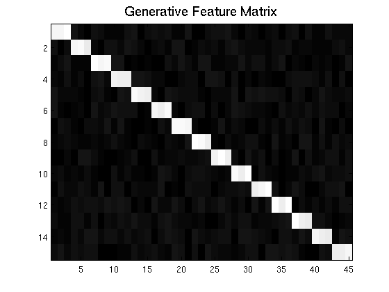
(a) True A

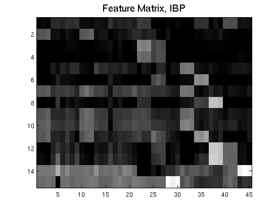
(b) IBP A

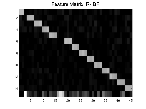
(c) R-IBP A

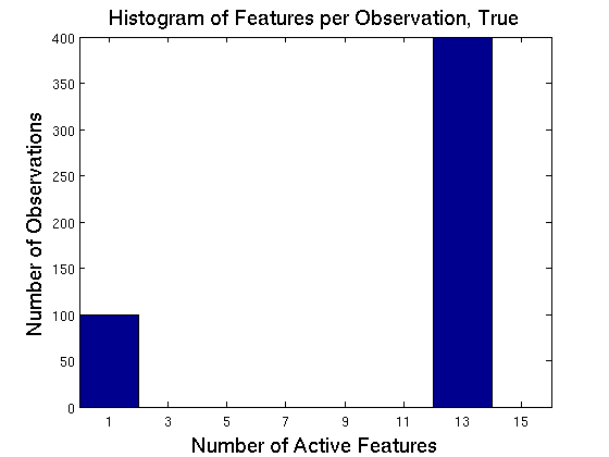
(d) True Histogram over active features per observation

(e) IBP Histogram over active features per observation

(f) R-IBP Histogram over active features per observation

Figure 5: Examples of features and counts of active features found by the variational inference for the R-IBP and the IBP on the toy data. The R-IBP recovers patterns much closer to the true features than the IBP, in which observations with just one feature tend to get assigned no features, while observations with many get a few generic features corresponding to most dimensions being active. In contrast, the R-IBP recovers a histogram of features per observation that is much closer to the true distribution.

7.1.2 Knowledge about the Feature Distribution Assists with Predictive Performance

While interpretable features are desirable, we do not want them to come at the expense of predictive performance. To evaluate predictive performance, we considered 500 observations from a one-inflated Poisson model in which 80% of the observations have one associated latent feature and the remaining 20% have a Poisson-distributed number of associated latent features with mean $\lambda$. Such a model might be relevant when modeling patients in a typical clinical practice, where most patients might have very simple complaints and a few patients may have a very complex combination of diseases. We apply the Gibbs sampler for $\lambda=\{3,6,9,12\}$; the concentration parameter for the IBP was set to the mean number of features per observation in each setting.

We explore two variants of the R-IBP: in the fully exchangeable version, we know that observations come from a mixture distribution but we do not know whether the observation is associated with the spike or the slab; all observations have the same $f_{n}=0.8\delta_{1}+0.2\mbox{Poisson}(\lambda)$. In the partially exchangeable version, we know to which mixture component the observation belongs. If the observation belongs to the spike, we have $f_{n}=\delta_{1}$, otherwise we have $f_{n}=\mbox{Poisson}(\lambda)$ This assumption may be reasonable in many domains; for example, it may be easy to tell if a patient has a simple or complex condition without knowing explicitly what diseases a patient with complex diseases has.

We randomly held out 1% of the data. Figure 6 shows the negative log-likelihoods on the held-out data averaged over 5 runs of 500 iterations each (lower is better). When the mean number latent features in the slab distribution $\lambda=3$, all observations have few features, and the R-IBP variants performs slightly worse than the IBP – something we attribute to slower mixing and therefore slower convergence, due to the lack of conjugacy. However, as the slab mean $\lambda$ increases, the R-IBPs variants consistently out-perform the IBP. As expected, the partially-exchangeable variant, in which each observation contains a covariate describing whether it is a member of the spike or the slab, does the best.

Figure 6: Negative log-likelihoods (lower is better) for data from a one-inflated Poisson model with the mean of the Poisson $\lambda=\{3,6,9,12\}$. R-IBP is the fully exchangeable R-IBP model, whereas R-IBP-PE is the partially-exchangeable R-IBP model where each observation is associated with a covariate describing from which distribution it comes.

7.2 Comparison on Multiple Real Data Sets

We compare the two inference approaches for the R-IBP from sections 6.1 and 6.2 to three IBP baselines. The hybrid variational IBP applies the same hybrid variational approach to inference in the IBP as was developed for the R-IBP in section 6.2. We also compare to Gibbs sampling in the IBP Griffiths and Ghahramani, (2011) and the standard variational inference approach for the IBP Doshi et al., (2009). In all cases, we the linear Gaussian likelihood model in which the data $X$ are assumed to be generated by $ZA+\epsilon$, where $A$ is an $I\times D$ feature matrix with independent normal priors $\mbox{Normal}(0,\sigma_{A}^{2})$ on each value and $\epsilon$ is a $N\times D$ matrix of independent noise drawn from $\mbox{Normal}(0,\sigma_{n}^{2})$. Both the Gibbs sampler and the variational methods were run for 300 iterations. For the hybrid variational methods, the weights were resampled every 25 iterations of the coordinate ascent. All methods were run 5 times. A random 1% of the data was held-out for evaluation.

We compare these methods on several data sets:

• The chord data set consists of a collection of three-note chords and single notes. All 1320 three-note permutations and all 12 single notes for the octave containing middle C were synthesized into wav files using MIDIUtil and FluidSynth; the power spectrum of these wav files was evaluated at every 10Hz between 0 and 1000Hz, resulting in a dataset with 100 dimensions. For the R-IBP, we used the partially exchangeable version, where we provided information stating that single notes had 1 latent feature in expectation $(k_{n}=1)$ and chords had 3 latent features in expectation ($k_{n}=3)$.

• The newsgroup data-set is the subset of the 20 newsgroups data set from http://www.cs.nyu.edu/ roweis/data.html, consisting of the counts for the top 100 words for 5000 documents. We arbitrarily set $k_{n}=\frac{L_{n}}{150}$, where $L_{n}$ was the length of the document.

• The NPR data set consisted of the 365 features and the 365 summaries from April 2013 to April 2014. The stories were processed through NLTK clean and we kept the 1964 most common words. We provided the information that the expected number of topics in a features story was $k_{n}=1$ while the expected number of topics in a summary was $k_{n}=5$.

In all cases, the distribution $f$ was set to be uniform over $k_{n}\pm 1$. We used a linear Gaussian likelihood in all cases.

Likelihoods and training times for the toy problem and other problems are shown in tables 1, 2 and 3. Here we see that the auxiliary information provided by the R-IBP also translates into better likelihoods and not just qualitatively better parameter recovery. As expected, the variational inference also runs significantly faster than the MCMC-based approaches; however in some of the experiments the variational approach yielded a lower quality estimate (shown most clearly in the NPR dataset).

Table 1: Comparison of training set likelihoods for the R-IBP and the IBP.

	Chord	Newsgroups	NPR
Hybrid-Var.	-1.25e+05	-2.33e+06	-1.65e+07
R-IBP	(-1.25e+05, -1.25e+05)	(-2.33e+06, -2.33e+06)	(-1.66e+07, -1.65e+07)
Hybrid-Var.	-2.13e+05	-2.38e+06	-6.49e+06
IBP	(-2.13e+05, -2.13e+05)	(-2.38e+06, -2.38e+06)	(-6.50e+06, -6.48e+06)
Variational	-2.13e+05	-2.39e+06	-6.90e+06
IBP	(-2.13e+05, -2.13e+05)	(-2.39e+06, -2.39e+06)	(-6.96e+06, -6.83e+06)
Gibbs R-IBP	-1.33e+05	-2.34e+06	-4.89e+06
	(-1.33e+05, -1.33e+05)	(-2.34e+06, -2.34e+06)	(-4.90e+06, -4.89e+06)
Gibbs IBP	-1.25e+05	-2.34e+06	-5.15e+06
	(-1.25e+05, -1.25e+05)	(-2.34e+06, -2.34e+06)	(-5.16e+06, -5.14e+06)

Table 2: Comparison of test set likelihoods for the R-IBP and the IBP.

	Chord	Newsgroups	NPR
Hybrid-Var.	-2.11e+03	-2.38e+04	-1.77e+05
R-IBP	(-2.13e+03, -2.09e+03)	(-2.38e+04, -2.37e+04)	(-1.80e+05, -1.74e+05)
Hybrid-Var.	-2.12e+03	-2.43e+04	-7.07e+04
IBP	(-2.13e+03, -2.11e+03)	(-2.43e+04, -2.42e+04)	(-7.14e+04, -7.00e+04)
Variational	-2.12e+03	-2.43e+04	-7.28e+04
IBP	(-2.13e+03, -2.11e+03)	(-2.43e+04, -2.42e+04)	(-7.33e+04, -7.22e+04)
Gibbs R-IBP	-2.26e+03	-2.37e+04	-5.46e+04
	(-2.29e+03, -2.24e+03)	(-2.37e+04, -2.37e+04)	(-5.48e+04, -5.44e+04)
Gibbs IBP	-2.32e+03	-2.37e+04	-5.79e+04
	(-2.34e+03, -2.29e+03)	(-2.38e+04, -2.37e+04)	(-5.81e+04, -5.77e+04)

Table 3: Comparison of running times (in seconds) for the R-IBP and the IBP.

	Chord	Newsgroups	NPR
Hybrid-Var.	1.43e+03	1.56e+05	1.02e+04
R-IBP	(1.42e+03, 1.44e+03)	(1.55e+05, 1.58e+05)	(1.01e+04, 1.02e+04)
Hybrid-Var.	9.68e+02	3.21e+04	1.65e+04
IBP	(9.60e+02, 9.76e+02)	(3.19e+04, 3.23e+04)	(1.63e+04, 1.66e+04)
Variational	1.05e+03	3.69e+04	1.50e+04
IBP	(1.04e+03, 1.06e+03)	(3.67e+04, 3.72e+04)	(1.49e+04, 1.50e+04)
Gibbs R-IBP	3.56e+03	2.04e+04	9.97e+03
	(3.52e+03, 3.60e+03)	(1.99e+04, 2.08e+04)	(9.70e+03, 1.02e+04)
Gibbs IBP	2.01e+03	1.33e+04	7.39e+03
	(1.99e+03, 2.02e+03)	(1.31e+04, 1.35e+04)	(7.20e+03, 7.58e+03)

8 Discussion and Future Work

The Restricted Indian Buffet Process is a useful tool for latent feature modeling with a non-Poissonian number of latent features per data point. In this article, we have expanded on the original exposition Williamson et al., (2013) by providing new representations that connect the R-IBP to tilted CRMs and the scaled beta-prime process. We also provide several alternatives for exact and approximate simulation from the R-IBP, as well as new inference algorithms, including a computationally efficient variational/MCMC hybrid algorithm.

While the IBP often has reasonable performance on data sets with arbitrary distributions over the number of features—rather than a Poisson distribution—we find that additional knowledge about the number of features can be very helpful if it is available. In particular, a common challenge when performing inference with the IBP is that it often learns combinations of features as a single feature, especially when there are correlations between features. While these feature combinations may reasonably represent the data, a latent variable model that learns such grouped features will do poorly if asked to make predictions on observations where that correlation is not present. With the R-IBP, it is possible to specify the expected number of features in an observation, allowing us to discover features with both better interpretability and generalization.

In general, we see the most pronounced differences in situations where we had strong prior knowledge about the number of features in a dataset—such as the chord and toy examples. Differences were less pronounced in data sets such as newsgroups, where we made somewhat arbitrary decisions about the potential number of features based on document lengths; in general the IBP is a sufficiently flexible prior to capture posteriors with relatively small deviations from Poisson-distributions on the number of latent features, and in this case we actively decreased this flexibility. An interesting direction for further research would be try to leverage less strong prior information—such as the information in the NPR data set where some stories are features and some stories are collections of multiple news summaries.

More broadly, while we have focused on the Indian Buffet Process, the concepts described in this paper are applicable to other nonparametric models such as the beta-negative Binomial process or gamma-Poisson process. As we discussed in Section 4, the variety of possible restrictions is much broader when considering non-binary matrices, which are often used for modeling count data. It will be interesting to explore where restricted models can be effectively used in this context; in principle different restrictions can allow domain experts to encode a rich number of kinds of prior knowledge.

Finally, there is much to be explored on approaches for incorporating the kinds of observation-specific restrictions described in this work. The R-IBP has a natural interpretation as an IBP with arbitrary distributions on the number of features in each observation. However, as we discussed in Section 3.4, there is an extra degree of freedom when we specify the Restricted IBP with a beta process or a beta-prime process. Intuitively, this invariance arises because conditioned on the number of latent features in an observation, the scale of the weights no longer matters. Any restriction that can be viewed as conditioning will result in this property. In theory, working with a normalized beta-prime process would remove this invariance; in practice, working with a normalized beta-prime process is intractable.

However, there do exist other tractable normalized random measures James et al., (2009) such as the Dirichlet process and other and nonparametric probability measures such as the Pitman-Yor process Pitman and Yor, (1997). These measures could be substituted for the beta-prime process in Equation 8. The resulting model could no longer be interpreted as a restricted version of the IBP, but it is nonetheless a valid model that may have very similar properties. Having a more potentially more tractable directing measure may assist in developing robust and scalable inference techniques for restricted models.