Bifurcations of the Lagrangian orbits from the classical to the curved 3-body problem

Abstract.

We consider the 3-body problem of celestial mechanics in Euclidean, elliptic, and hyperbolic spaces, and study how the Lagrangian (equilateral) relative equilibria bifurcate when the Gaussian curvature varies. We thus prove the existence of new classes of orbits. In particular, we find some families of isosceles triangles, which occur in elliptic space.

Florin Diacu
Pacific Institute for the Mathematical Sciences
and
Department of Mathematics and Statistics
University of Victoria
Victoria, Canada
Email: diacu@uvic.ca

1. Introduction

The idea of extending Newtonian gravitation to spaces of constant curvature appeared for the first time in the work of János Bolyai and Nikolai Lobachevsky, who independently considered it in the framework of hyperbolic geometry, [2], [26]. They apparently thought in terms of Gauss’s flux law for gravity, according to which two celestial bodies attract each other with a force inversely proportional to the area of a sphere of radius equal to the distance between the bodies.

As it happened to their work in hyperbolic geometry, it took many years until the research community recognized the importance of studying the motion of point masses gravitating in spaces of constant curvature. Lejeune Dirichlet apparently grasped the value of this problem in the 1850s, but in spite of researching it he published nothing in this direction, [31]. The first to write down the expression of the potential in hyperbolic space was Ernest Schering, almost four decades after Bolyai and Lobachevsky. In his derivation, Schering used the fact that the area of a sphere of radius $r$ in $\mathbb{H}_{\kappa}^{3}$ is $4\pi|\kappa|^{-1}\sinh^{2}(|\kappa|^{1/2}r)$, where $\mathbb{H}_{\kappa}^{3}$ denotes the hyperbolic space of curvature $\kappa<0$, [31], [32]. It was then natural to extend this problem to elliptic space, so Wilhelm Killing defined a force inversely proportional to the area $4\pi\kappa^{-1}\sin^{2}(\kappa^{1/2}r)$ of a sphere of radius $r$ in the complete elliptic geometry of the sphere $\mathbb{S}_{\kappa}^{3}$ of curvature $\kappa>0$, [20]. Currently, the topic is intensely researched thanks to the new approach initiated in [3], [13], and [14] (see also [4], [5], [6], [7], [8], [9], [10], [11], [12], [15], [16], [17], [19], [27], [28], [29], [33], [34], [35], [36], [37]).

To get more insight into the problem, let’s consider the motion of two point masses, $m_{1}$ and $m_{2}$, in the three existing kinds of spaces of constant curvature we are interested in, $\mathbb{H}_{\kappa}^{3}$ ($\kappa<0$), $\mathbb{R}^{3}$ ($\kappa=0$), and $\mathbb{S}_{\kappa}^{3}$ ($\kappa>0$), and assume that the corresponding hyperbolic, Euclidean, and elliptic distance between the point masses is a function $r=r(t)$. Let us take the units such that the gravitational constant is 1. Then the attracting forces are given by

$$F_{\mathbb{H}_{\kappa}^{3}}(r)=\frac{|\kappa|m_{1}m_{2}}{\sinh^{2}(|\kappa|^{1/2}r)},\ \ \ F_{\mathbb{R}^{3}}(r)=\frac{m_{1}m_{2}}{r^{2}},\ \ \ F_{\mathbb{S}_{\kappa}^{3}}(r)=\frac{\kappa m_{1}m_{2}}{\sin^{2}(\kappa^{1/2}r)}.$$

The corresponding force functions (the negatives of the potentials, whose derivatives relative to $r$ provide the above forces), take the form

$$V_{\mathbb{H}_{\kappa}^{3}}(r)=m_{1}m_{2}\coth(|\kappa|^{1/2}r),\ \ \ V_{\mathbb{R}^{3}}(r)=\frac{m_{1}m_{2}}{r},\ \ \ V_{\mathbb{S}_{\kappa}^{3}}(r)=m_{1}m_{2}\cot(\kappa^{1/2}r).$$

The classical Newtonian law is recovered in the limit since

$$\lim_{\kappa\to 0,\ \!\kappa<0}F_{\mathbb{H}_{\kappa}^{3}}(r)=\lim_{\kappa\to 0,\ \!\kappa>0}F_{\mathbb{S}_{\kappa}^{3}}(r)=F_{\mathbb{R}^{3}}(r),$$

and similar relationships stand true for the force functions.

But in spite of recovering the Newtonian law in the limit, how can we know that this is the most natural extension of gravity to spaces of constant curvature? After all, there are infinitely many ways of obtaining the classical force when $\kappa\to 0$. In the absence of any physical or observational tests, is Gauss’s law good enough reason for the introduction of the above definitions? Some researchers obviously believed it was not, for Rudolf Lipschitz came up with another expression of the force in curved space, [25]. His proposed law, however, was short lived. First, the solutions to his equations of motion involved elliptic integrals, so they could not be solved. Second, some strong arguments occurred in favour of the approach initiated by Bolyai and Lobachevsky. Indeed, at the beginning of the 20th century, Heinrich Liebmann proved two important results relative to the Kepler problem (which studies the motion of one body about a fixed attractive centre). The first was that, like in the Euclidean case, the potential is a harmonic function, i.e. a solution of the Laplace-Beltrami equation. The second property showed that all bounded orbits are closed, a result originally proved by Joseph Bertrand for the Newtonian force in Euclidean space, [1]. These reasons were convincing enough to accept, even though only on the basis of mathematical analogies and in the absence of physical experiments or observations, that the force functions $V_{\mathbb{H}^{3}}$ and $V_{\mathbb{S}^{3}}$ provide the correct extension of $V_{\mathbb{R}^{3}}$ to spaces of constant curvature. In fact, this conclusion should not be too surprising: Newton’s gravitational law does not shed any light on the physical nature of gravity, it only describes the motion of celestial bodies fairly well. But as we will further explain, the above generalization of the gravitational law may also have merits that transcend mathematics, although this is first of all a mathematical problem.

In 1821 Carl Friedrich Gauss performed some topographic measurements in which he measured the angles of a triangle formed by three mountain peaks, [6]. His aim was apparently to find out whether space was hyperbolic or elliptic, should the sum of the angles add to less or more than $\pi$ radians. His attempt was inconclusive since the measurement errors were above the potential deviation from $\pi$. Lobachevsky tried to decide whether the physical space was curved by measuring the parallax of Sirius, which he treated as the ideal point of an angle of parallelism, but he couldn’t draw any conclusion either. These and other 19th-century attempts to determine the curvature of space are described in [21]. In his famous 1854-paper that laid the foundations of differential geometry, Bernhard Riemann reiterated the importance of this problem, [30]. More recently the so-called boomerang experiment, involving the background radiation, was also initiated in the hope to answer this question, but again without success, [6]. All these efforts proved, however, that even if the large-scale universe is not Euclidean, the deviation from zero curvature, if any, must be extremely small.

The mathematical extension of gravitation to spaces of non-zero constant curvature offers another way to approach the problem of determining the curvature of the physical space. If, for instance, we could prove that certain orbits exist only in, say, Euclidean space, but not in hyperbolic and elliptic space, and we succeed to find these orbits through astronomical observations, then we would be able to conclude that the universe is flat. So the study of the $N$-body problem in spaces of constant Gaussian curvature (or curved $N$-body problem, as we informally call it), may present interest beyond mathematics.

2. Our goal

In the Newtonian 3-body problem of the Euclidean space there are two classes of relative equilibria, the Lagrangian and the Eulerian, named after those who proved their existence. Leonhard Euler found the collinear orbits in 1762, [18]. Joseph Louis Lagrange rediscovered them a decade later, but also found the class of relative equilibria given by equilateral triangles, [22]. In this paper we will study the latter type of solutions and analyze how they bifurcate from the Euclidean plane to 2-spheres and hyperbolic 2-spheres. The reason why we restrict our study to the 2-dimensional case is that all relative equilibria are planar in the Euclidean space. However, it is important to mention that in the curved problem there are relative equilibria that do not necessarily move on great 2-spheres or great hyperbolic 2-spheres, but this phenomenon can take place only for more than three bodies. In previous work, we provided such examples for the curved 3-dimensional problem, [5], [6], [9]. So when investigating the motion of more than three bodies, a 3-dimensional study would also be necessary. In this paper, however, we can restrict our considerations to the 2-dimensional case without any loss of generality.

It will be interesting to notice in the following sections that the dynamics on 2-spheres is richer than on hyperbolic 2-spheres, in the sense that there are more triangular relative equilibria on $\mathbb{S}_{\kappa}^{2}$ than on $\mathbb{H}_{\kappa}^{2}$. Perhaps one of the reasons for this difference can be found in the inequalities

$$\frac{1}{\sinh^{2}r}<\frac{1}{r^{2}}<\frac{1}{\sin^{2}r},$$

which imply that

$$F_{\mathbb{H}_{\kappa}^{2}}<F_{\mathbb{R}^{2}}<F_{\mathbb{S}_{\kappa}^{2}},$$

so the component of the force derived from the potential (since, for $\kappa\neq 0$, the acceleration also involves the force due to the constraints, which keep the bodies on the manifolds) is stronger on spheres than on hyperbolic spheres.

3. Summary of the results

After introducing the equations of motion in Section 4, we study in Section 5 the existence of relative equilibria on and near the equator of $\mathbb{S}_{\kappa}^{2}$. Our first theorem provides a different proof for a result we first published in [4], namely that for every acute scalene triangle inscribed in the equator, we can find a class of masses $m_{1},m_{2},m_{3}>0$, which if placed at the vertices of the triangle form a relative equilibrium that rotates around the equator with any chosen nonzero angular velocity. Then in Theorem 2 we prove a qualitative property: if the three bodies move either in the northern or in the southern closed hemisphere and one of the bodies is on the equator, then all three bodies must move on the equator. In Theorem 3, we find new classes of relative equilibria that move on non-great circles parallel with the plane of the equator, namely those given by isosceles non-equilateral triangles. These relative equilibria occur for masses $m_{1}=:M>0$ and $m_{2}=m_{3}=:m>0$, with $M<2m$, in two pairs of bands symmetric to the equator, as shown in Figure 2. For one of the classes the shape of the isosceles triangle is unique for the given masses, whereas in the other class two distinct shapes are possible. For $M=m$ we recover the Lagrangian (equilateral) relative equilibria, which exist on all circles parallel with (and including) the equator, a result we first proved in [13].

In Section 6 we study the existence of relative equilibria parallel with the $xy$-plane in $\mathbb{H}_{\kappa}^{2}$. We witness here the first manifestation of the difference between the richness of orbits that occur on spheres and hyperbolic spheres by proving that there are no isosceles relative equilibria parallel with the $xy$-plane other than the Lagrangian solutions of equal masses. In Section 7 we introduce some equivalent form of the equations of motion that is more suitable for the study of Lagrangian (equilateral) relative equilibria. This form of the equations has been suggested to us by Carles Simó, who used them in a recent paper on the restricted curved 3-body problem he wrote with Regina Martínez, [28]. In Section 8 we take a glimpse at the simple case of the planetary problem, in which two masses are negligible, and prove in Theorem 5 that there occur no bifurcations of the Lagrangian relative equilibria when passing from $\mathbb{S}_{\kappa}^{2}$ to $\mathbb{R}^{2}$ to $\mathbb{H}_{\kappa}^{2}$ as kappa goes from $+\infty$ to $-\infty$.

In Section 9 we focus on the case of one negligible mass. In Theorem 6 we assume that two bodies of equal mass move on a non-equatorial circle of the sphere $\mathbb{S}_{\kappa}^{2}$, being always diametrically opposed, and form a Lagrangian relative equilibrium with a third body, which has negligible mass. Then the circle on which the two bodies move must have its radius equal to $(2\kappa)^{-1/2}$ and the third body must move on the equator. In other words, given $\kappa$, the size of the equilateral triangle does not depend on the value of the equal masses, but the angular velocity of the equilateral triangle does. In Theorem 7 we then show that there are no Lagrangian relative equilibria in $\mathbb{H}_{\kappa}^{2}$ with two bodies of equal mass and a third body of negligible mass, finding again a manifestation of the difference between the richness of orbits that occur on spheres and hyperbolic spheres. Finally in Theorem 8 we show that if one of the three masses is negligible, then there are no Lagrangian relative equilibria in $\mathbb{H}_{\kappa}^{2}$ and there are no Lagrangian relative equilibria in $\mathbb{S}_{\kappa}^{2}$ either if the curvature $\kappa$ is sufficiently small, unless the two non-negligible masses are equal, in which case the orbits occur as stated in Theorem 6.

4. Equations of motion

The goal of this section is to define the spaces of constant curvature in which the bodies move and introduce the equations of motion that extend Newton’s classical system beyond the Euclidean case. Consider for this the family of 2-dimensional manifolds $(\mathbb{M}_{\kappa}^{2})_{\kappa\in\mathbb{R}}$, with

$$\mathbb{M}_{\kappa}=\begin{cases}\mathbb{S}_{\kappa}^{2}\hskip 8.5359pt{\rm for}\ \ \kappa>0\cr\mathbb{R}^{2}\hskip 7.11317pt{\rm for}\ \ \kappa=0\cr\mathbb{H}_{\kappa}^{2}\hskip 5.97527pt{\rm for}\ \ \kappa<0,\end{cases}$$

where the set $\mathbb{R}^{2}$ is the horizontal Euclidean plane of curvature $\kappa=0$ through the origin of the coordinate system,

$$\mathbb{R}^{2}=\{(x,y,z)\ \!|\ \!z=0\},$$

the sets $\mathbb{S}_{\kappa}^{2}$ denote the spheres

$$\mathbb{S}_{\kappa}^{2}=\{(x,y,z)\ \!|\ \!\kappa(x^{2}+y^{2}+z^{2})+2\kappa^{1/2}z=0\}$$

centred at $(0,0,-\kappa^{-1/2})$ of curvature $\kappa>0$, and the sets $\mathbb{H}_{\kappa}^{2}$ are the hyperbolic spheres of curvature $\kappa<0$ represented by the upper sheets of hyperboloids of two sheets,

$$\mathbb{H}_{\kappa}^{2}=\{(x,y,z)\ \!|\ \!\kappa(x^{2}+y^{2}-z^{2})+2|\kappa|^{1/2}z=0,\ z\geq 0\},$$

whose vertex is tangent to the $xy$-plane. The spheres $\mathbb{S}_{\kappa}^{2}$ and the plane $\mathbb{R}^{2}$ are embedded in $\mathbb{R}^{3}$, which has the standard inner product of signature $(+,+,+)$, whereas $\mathbb{H}_{\kappa}^{3}$ is embedded in the Minkowski space $\mathbb{R}^{2,1}$, endowed with the Lorentz inner product of signature $(+,+,-)$. All these manifolds have a single point in common, the origin $(0,0,0)$ of the coordinate system (see Figure 1).

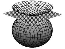
Figure 1. A snapshot of the continuous transition from the spheres $\mathbb{S}_{\kappa}^{2}$, of constant curvature $\kappa>0$, to the plane $\mathbb{R}^{2}$, of curvature $\kappa=0$, and to the hyperbolic spheres $\mathbb{H}_{\kappa}^{2}$, of curvature $\kappa<0$, as $\kappa$ decreases from $+\infty$ to $-\infty$.

In a previous paper, [8], we obtained the equations of motion of the $N$-body problem on the above 2-dimensional manifolds of constant curvature as well as in their 3-dimensional counterparts. But here we will consider only the case $N=3$ on $\mathbb{M}_{\kappa}^{2}$. Then the equations of motion have the form

(1) $$\begin{cases}\ddot{x}_{i}=\sum_{j=1,j\neq i}^{3}\frac{m_{j}\Big{[}x_{j}-\Big{(}1-\frac{\kappa r_{ij}^{2}}{2}\Big{)}x_{i}\Big{]}}{r_{ij}^{3}\Big{(}1-\frac{\kappa r_{ij}^{2}}{4}\Big{)}^{3/2}}-\kappa(\dot{\bf r}_{i}\cdot\dot{\bf r}_{i})x_{i}\cr\ddot{y}_{i}=\sum_{j=1,j\neq i}^{3}\frac{m_{j}\Big{[}y_{j}-\Big{(}1-\frac{\kappa r_{ij}^{2}}{2}\Big{)}y_{i}\Big{]}}{r_{ij}^{3}\Big{(}1-\frac{\kappa r_{ij}^{2}}{4}\Big{)}^{3/2}}-\kappa(\dot{\bf r}_{i}\cdot\dot{\bf r}_{i})y_{i}\cr\ddot{z}_{i}=\sum_{j=1,j\neq i}^{3}\frac{m_{j}\Big{[}z_{j}-\Big{(}1-\frac{\kappa r_{ij}^{2}}{2}\Big{)}z_{i}+\frac{\sigma|\kappa|^{1/2}r_{ij}^{2}}{2}\Big{]}}{r_{ij}^{3}\Big{(}1-\frac{\kappa r_{ij}^{2}}{4}\Big{)}^{3/2}}-(\dot{\bf r}_{i}\cdot\dot{\bf r}_{i})(\kappa z_{i}+\sigma|\kappa|^{1/2}),\end{cases}$$

$i=1,2,3$, where $m_{1},m_{2},m_{3}>0$ represent the masses,

$${\bf r}_{i}=(x_{i},y_{i},z_{i}),\ \ \dot{\bf r}_{i}=(\dot{x}_{i},\dot{y}_{i},\dot{z}_{i}),\ i=1,2,3,$$

are, respectively, the position vectors and the velocities of the bodies, $\sigma$ denotes the signum function: $\sigma=+1$ for $\kappa\geq 0$ and $\sigma=-1$ for $\kappa<0$, and

$$r_{ij}:=[(x_{i}-x_{j})^{2}+(y_{i}-y_{j})^{2}+\sigma(z_{i}-z_{j})^{2}]^{1/2},\ \ i,j=1,2,3,$$

is the Euclidean distance between the bodies of masses $m_{i}$ and $m_{j}$ in $\mathbb{R}^{3}$, but the Minkowski distance in $\mathbb{R}^{2,1}$.

At $t=0$, the initial conditions must have the six constraints

(2) $$\kappa(x_{i}^{2}+y_{i}^{2}+\sigma z_{i}^{2})+2|\kappa|^{1/2}z_{i}=0,\ \ i=1,2,3,$$

(3) $$\kappa{\bf r}_{i}\cdot\dot{\bf r}_{i}+|\kappa|^{1/2}\dot{z}_{i}=0,\ \ i=1,2,3.$$

Since the sets $\mathbb{S}_{\kappa}^{2}$ and $\mathbb{H}_{\kappa}^{2}$ are invariant for the above equations of motion, these conditions are satisfied for all $t$. They are identically satisfied on $\mathbb{R}^{2}$, i.e. for $\kappa=0$.

Let us take a value of $\kappa$ and fix the point masses $m_{i}$ and $m_{j}$ on the manifold $\mathbb{M}_{\kappa}^{2}$. If we let $\kappa$ vary and keep $r_{ij}$ constant, then the coordinates of the point masses vary with $\kappa$. In particular, the values of $z_{i},\ i=1,2,3$, and consequently the values of the expressions $(z_{i}-z_{j})^{2},\ i,j=1,2,3,i\neq j,$ become small when $\kappa$ gets close to 0 and vanish at $\kappa=0$. Consequently, for $\kappa=0$ we recover the classical Newtonian equations of the $3$-body problem in the Euclidean plane,

(4) $$\ddot{\bf r}_{i}=\sum_{j=1,j\neq i}^{3}\frac{m_{j}({\bf r}_{j}-{\bf r}_{i})}{r_{ij}^{3}},\ \ i=1,2,3,$$

where ${\bf r}_{i}=(x_{i},y_{i},0),\ i=1,2,3$.

5. Relative equilibria on and near the equator of $\mathbb{S}_{\kappa}^{2}$

In this section we will introduce some coordinates that allow us to better detect relative equilibria on and near the equator of $\mathbb{S}_{\kappa}^{2}$, namely $(\varphi,\omega)$, where $\varphi$ measures the angle from the $x$-axis in the $xy$-plane and $\omega$ is the height on the vertical $z$-axis. To express the coordinates of each body in this way, let us remark that from the constraints (2), which can be written on $\mathbb{S}_{\kappa}^{2}$ as

$$x_{i}^{2}+y_{i}^{2}+\omega_{i}^{2}+2\kappa^{-1/2}\omega_{i}=0,\ i=1,2,3,$$

we obtain the relations

$$\Omega_{i}:=x_{i}^{2}+y_{i}^{2}=-\kappa^{-1/2}\omega_{i}(\kappa^{1/2}\omega_{i}+2)\geq 0,\ \ i=1,2,3.$$

Notice that in the inequality, which follows from the fact that $\omega_{i}\in[-2\kappa^{-1/2},0]$, equality occurs only when the body is at the North or South Pole.

We can now express the positions of the bodies in $(\varphi,\omega)$-coordinates with the help of the polar transformations

$$x_{i}=\Omega_{i}^{1/2}\cos\varphi_{i},\ \ y_{i}=\Omega_{i}^{1/2}\sin\varphi_{i},\ \ i=1,2,3.$$

Some straightforward computations show that the equations of motion (1) take the form

(5) $$\begin{cases}\ddot{\varphi}_{i}=\Omega_{i}^{-1/2}\sum_{j=1,j\neq i}^{3}\frac{m_{j}\Omega_{j}^{1/2}\sin(\varphi_{j}-\varphi_{i})}{\rho_{ij}^{3}\big{(}1-\frac{\kappa\rho_{ij}^{2}}{4}\big{)}^{3/2}}-\frac{\dot{\varphi}_{i}\dot{\Omega}_{i}}{\Omega_{i}}\cr\ddot{\omega}_{i}=\sum_{j=1,j\neq i}^{3}\frac{m_{j}\big{[}\omega_{j}-\omega_{i}+\frac{\kappa\rho_{ij}^{2}}{2}(\omega_{i}+\kappa^{-1/2})\big{]}}{\rho_{ij}^{3}\big{(}1-\frac{\kappa\rho_{ij}^{2}}{4}\big{)}^{3/2}}-(\kappa\omega_{i}+\kappa^{\frac{1}{2}})\big{(}\frac{\dot{\Omega}_{i}^{2}}{4\Omega_{i}}+\dot{\varphi}_{i}^{2}\Omega_{i}+\dot{\omega}_{i}^{2}\big{)},\end{cases}$$

$i=1,2,3$, where

$$\dot{\Omega}_{i}=-2\kappa^{-1/2}\dot{\omega}_{i}(\kappa^{1/2}\omega_{i}+1),\ \ i=1,2,3,$$

$$\rho_{ij}^{2}=\Omega_{i}+\Omega_{j}-2\Omega_{i}^{1/2}\Omega_{j}^{1/2}\cos(\varphi_{i}-\varphi_{j})+(\omega_{i}-\omega_{j})^{2},\ i,j=1,2,3,\ i\neq j.$$

5.1. Relative equilibria on the equator

Let us first seek relative equilibria on the equator $\omega=-\kappa^{-1/2}.$ Then

$$\omega_{i}=-\kappa^{-1/2},\ \ \dot{\omega}_{i}=0,\ \ \Omega_{i}=\kappa^{-1},\ \ \dot{\Omega}_{i}=0,\ \ i=1,2,3,$$

$$\rho_{ij}^{2}=2\kappa^{-1}[1-\cos(\varphi_{i}-\varphi_{j})],\ i,j=1,2,3,\ i\neq j.$$

In this case, the equations in (5) corresponding to $\ddot{\omega}_{i},\ i=1,2,3$, are identically satisfied, and the equations corresponding to $\ddot{\varphi}_{i},\ i=1,2,3$, lead to the system

(6) $$\ddot{\varphi}_{i}=\kappa^{3/2}\sum_{j=1,j\neq i}^{3}\frac{m_{j}\sin(\varphi_{j}-\varphi_{i})}{|\sin(\varphi_{j}-\varphi_{i})|^{3}},\ \ i=1,2,3.$$

But for relative equilibria the angular velocity is the same constant for all particles, so if we denote this velocity by $\alpha\neq 0$ we can assume that

(7) $$\varphi_{1}=\alpha t+a_{1},\ \varphi_{2}=\alpha t+a_{2},\ \varphi_{3}=\alpha t+a_{3},$$

where $t$ represents the time and $a_{1},a_{2},a_{3}$ are real constants. Therefore

$$\ddot{\varphi}_{i}=0,\ \ i=1,2,3.$$

With the notation

$$s_{1}:=\frac{\kappa^{3/2}\sin(\varphi_{1}-\varphi_{2})}{|\sin(\varphi_{1}-\varphi_{2})|^{3}},\ \ s_{2}:=\frac{\kappa^{3/2}\sin(\varphi_{2}-\varphi_{3})}{|\sin(\varphi_{2}-\varphi_{3})|^{3}},\ \ s_{3}:=\frac{\kappa^{3/2}\sin(\varphi_{3}-\varphi_{1})}{|\sin(\varphi_{3}-\varphi_{1})|^{3}},$$

which are constants, equations (6) take the form

(8) $$\begin{cases}\ \ \ \!m_{1}s_{1}-m_{3}s_{2}\ \ \ \ \ \ \ \ \ \ \ =0\cr-m_{2}s_{1}\ \ \ \ \ \ \ \ \ \ \ +m_{3}s_{3}\hskip 0.85358pt=0\cr\ \ \ \ \ \ \ \ \ \ \ \ \ \ \!m_{2}s_{2}-m_{1}s_{3}\hskip 0.56905pt=0.\end{cases}$$

This system has infinitely many solutions,

$$s_{1}=\frac{m_{3}}{m_{2}}\gamma,\ \ s_{2}=\frac{m_{1}}{m_{2}}\gamma,\ \ s_{3}=\gamma,$$

with $\gamma\neq 0$, such that $s_{1},s_{2},s_{3}$ make sense. We have thus obtained a new proof for a result we previously published in [4]:

Theorem 1.

For every acute scalene triangle inscribed in the equator of $\mathbb{S}_{\kappa}^{2}$, we can find a class of masses $m_{1},m_{2},m_{3}>0$, which if placed at the vertices of the triangle form a relative equilibrium that rotates around the equator with any chosen nonzero angular velocity.

It is interesting to note that for relative equilibria on $\mathbb{S}_{\kappa}^{2}$ if one body moves on the equator, then all bodies must move on the equator, as long as the bodies are assumed to move only in the upper, or only in the lower, closed hemisphere (i.e. including the equator). Let us now formally state and prove this result.

Theorem 2.

Consider a relative equilibrium on $\mathbb{S}_{\kappa}^{2}$ for which all the bodies move either in the northern or in the southern closed hemisphere. Then if one of the bodies moves on the equator, all the bodies move on the equator.

Proof.

Assume, without loss of generality, that the bodies are in the upper closed hemisphere, i.e.

$$\omega_{1}=-\kappa^{-1/2},\ \ \omega_{2}=-u,\ \ \omega_{2}=-v,\ \ u,v\in[0,\kappa^{-1/2}].$$

Then the equation in (5) corresponding to $\ddot{\omega}_{1}$ reduces to

$$\frac{m_{2}(\kappa^{-1/2}-u)}{\rho_{12}^{3}\Big{(}1-\frac{\kappa\rho_{12}^{2}}{4}\Big{)}^{3/2}}+\frac{m_{3}(\kappa^{-1/2}-v)}{\rho_{13}^{3}\Big{(}1-\frac{\kappa\rho_{13}^{2}}{4}\Big{)}^{3/2}}=0.$$

Since the masses and denominators in the left hand side of the above equation are positive and $0\leq u,v\leq\kappa^{-1/2}$, it follows that this equation can be satisfied only if $u=v=\kappa^{-1/2}$. Consequently all the bodies move on the equator. ∎

Remark 1.

The generalization of the above statement and proof to any number $N\geq 3$ of bodies is straightforward.

5.2. Relative equilibria parallel with the equator

In this subsection we will prove the existence of some isosceles relative equilibria that rotate on non-geodesic circles parallel with the plane of the equator. Here is the precise statement of our result.

Theorem 3.

For any sphere $\mathbb{S}_{\kappa}^{2}$ and masses $m_{1}=:M>0,m_{2}=m_{3}=:m>0$, with $M<2m$, there exist two non-geodesic circles parallel with the plane of the equator, symmetrically placed at distance $r\kappa^{-1/2}$ from it, such that the three bodies can form isosceles, non-equilateral, relative equilibria that rotate on any of those parallel circles. Moreover (see Figure 2),

(i) the shape of the triangle is unique if $r\in(0,\sqrt{3}/3]\cup\{3/5\}$,

(ii) there are two possible shapes of the triangle if $r\in(\sqrt{3}/3,3/5)$.

In each case the rotation takes place with constant nonzero angular velocity, whose value depends on $\kappa,m$, and $M$.

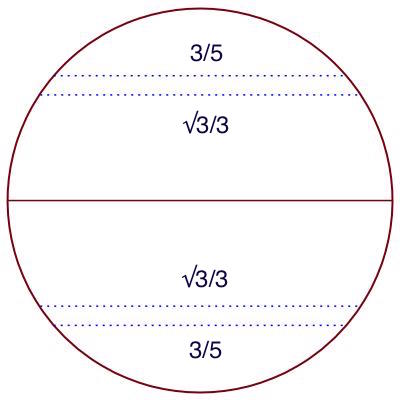
Figure 2. The zones in which one or two isosceles relative equilibria show up. The former orbits occur on the parallels marked by $3/5$ and in the large bands between the equator and the parallels marked by $\sqrt{3}/3$, whereas the latter show up in the two narrow bands, each between the parallel lines marked by $\sqrt{3}/3$ and $3/5$. The represented numbers, multiplied by $\kappa^{-1/2}$, which is the length of the sphere’s radius, give the distances of the dotted lines from the plane of the equator.

Proof.

We will start by seeking relative equilibria on non-great circles parallel with the equator. For this, we take

(9) $$\omega_{i}=-u\ ({\rm constant}),\ i=1,2,3,\ \ 0<u<2\kappa^{-1/2},\ u\neq\kappa^{-1/2}.$$

Then we have

$$\Omega_{i}=u(2\kappa^{-1/2}-u),\ \ \dot{\omega}_{i}=\dot{\Omega}_{i}=0,\ \ i=1,2,3,$$

and assuming that the $\varphi$-angular positions are given by the expressions in (7), we obtain that

$$\rho_{ij}^{2}=2u(2\kappa^{-1/2}-u)[1-\cos(a_{j}-a_{i})],\ \ i,j=1,2,3,\ i\neq j.$$

The equations corresponding to $\ddot{\omega}_{i},\ i=1,2,3,$ in system (5) reduce to the algebraic equations

$$\frac{\kappa(\kappa^{-1/2}-u)}{2}\Bigg{[}\sum_{j=1,j\neq i}\frac{m_{j}}{\rho_{ij}\big{(}1-\frac{\kappa\rho_{ij}^{2}}{4}\big{)}^{3/2}}-2\alpha^{2}u(2\kappa^{-1/2}-u)\Bigg{]}=0,\ \ i=1,2,3.$$

Since $\kappa>0$, we are not on the equator, i.e. $u\neq\kappa^{-1/2}$, and $\alpha^{2}$ must be the same in all the above three equations, this system leads to the conclusion that

(10) $$\frac{m_{2}}{A_{21}^{1/2}B_{21}^{3/2}}+\frac{m_{3}}{A_{31}^{1/2}B_{31}^{3/2}}=\frac{m_{1}}{A_{12}^{1/2}B_{12}^{3/2}}+\frac{m_{3}}{A_{32}^{1/2}B_{32}^{3/2}}=\frac{m_{1}}{A_{13}^{1/2}B_{13}^{3/2}}+\frac{m_{2}}{A_{23}^{1/2}B_{23}^{3/2}},$$

where

$$A_{ij}=1-\cos(a_{i}-a_{j}),\ \ B_{ij}=2-\gamma A_{ij},\ \ \gamma=\kappa u(2\kappa^{-1/2}-u).$$

Notice that $A_{ij}=A_{ji}$ and $B_{ij}=B_{ji},\ i,j=1,2,3,\ i\neq j$.

To evaluate the range in which $\gamma$ lies, we denote

$$u=\lambda\kappa^{-1/2},\ \ {\rm with}\ \ 0<\lambda<2,\ \lambda\neq 1,$$

in agreement with the conditions imposed on $u$ in (9). Then

$$\gamma=\lambda(2-\lambda),$$

which implies that, for the range of $\lambda$ specified above, we have

$$0<\gamma<1.$$

The equations corresponding to $\ddot{\varphi}_{i},\ i=1,2,3,$ in system (5) take the form

$$\sum_{j=1,j\neq i}^{3}\frac{m_{j}\sin(a_{j}-a_{i})}{\rho_{ij}^{3}\big{(}1-\frac{\kappa\rho_{ij}^{2}}{4}\big{)}^{3/2}}=0,\ \ i=1,2,3,$$

which are equivalent to

(11) $$\begin{cases}\cfrac{m_{2}\sin(a_{2}-a_{1})}{A_{21}^{3/2}B_{21}^{3/2}}+\cfrac{m_{3}\sin(a_{3}-a_{1})}{A_{31}^{3/2}B_{31}^{3/2}}=0\cr\cfrac{m_{1}\sin(a_{1}-a_{2})}{A_{12}^{3/2}B_{12}^{3/2}}+\cfrac{m_{3}\sin(a_{3}-a_{2})}{A_{32}^{3/2}B_{32}^{3/2}}=0\cr\cfrac{m_{1}\sin(a_{1}-a_{3})}{A_{13}^{3/2}B_{13}^{3/2}}+\cfrac{m_{2}\sin(a_{2}-a_{3})}{A_{23}^{3/2}B_{23}^{3/2}}=0.\end{cases}$$

It was shown in [13] that, for any given $u$ as above, there exist two values for the angular velocity $\alpha$, one corresponding to each sense of rotation, in the case when the triangle is equilateral and $m_{1}=m_{2}=m_{3}$. It is easy to see that we can recover these relative equilibria from equations (10) and (11). We will therefore look now for acute isosceles relative equilibria. Triangles with an obtuse angle cannot form relative equilibria since it is impossible to have relative equilibria if, at every moment in time, there is a plane containing the rotation axis such that all the bodies are on one side of it (see [13] for a proof of this fact). For this purpose, we can assume without loss of generality that

$$a_{1}=0,\ \ a_{2}=:a,\ \ a_{3}=:2\pi-a,\ \ {\rm with}\ \ a\in(\pi/2,\pi),$$

such that the isosceles triangle is acute. Then $A_{12}=A_{13}$ and $B_{12}=B_{13}$, so from the last equation in (10) we can draw the conclusion that $m_{2}=m_{3}$. Let us further use the notation

$$M:=m_{1},\ \ m:=m_{2}=m_{3}.$$

Then equations (10)-(11) reduce to

(12) $$\frac{2m-M}{A^{1/2}B^{3/2}}=\frac{m}{C^{1/2}D^{3/2}},$$

(13) $$\frac{M}{A^{3/2}B^{3/2}}=-\frac{2m\cos a}{C^{3/2}D^{3/2}},$$

respectively, where

$$A=1-\cos a,\ \ B=2-\gamma(1-\cos a),\ \ C=1-\cos 2a,\ \ D=2-\gamma(1-\cos 2a).$$

Expressing $A^{1/2}B^{3/2}$ in (12) in terms of $C^{1/2}D^{3/2}$ and substituting in (13), we are led to the conclusion that

$$\cos a=-\frac{M}{2m}.$$

Since $a\in(\pi/2,\pi)$, it means that

$$-1<-\frac{M}{2m}<0,$$

conditions that are satisfied for positive masses whenever

$$M<2m.$$

Notice that for $m=M$, equations (12)-(13) are identically satisfied, so we recover the Lagrangian equilateral relative equilibria.

Substituting $M=-2m\cos a$ in equations (12) and (13), we are led to the same relationship, namely

$$2-\gamma(1-\cos a)=4(1+\cos a)[1-\gamma(1-\cos^{2}a)].$$

Using the notation $s:=\cos a$, the above equation takes the form

$$4\gamma s^{3}+4\gamma s^{2}+(4-5\gamma)s-3\gamma+2=0,$$

which can be written as

$$\gamma=F(s),\ \ {\rm with}\ \ F(s)=-\frac{4s+2}{4s^{3}+4s^{2}-5s-3}.$$

It is easy to see that for $s\in(-1,-1/2)\cup(-1/2,0)$, $F$ takes values in the interval $[16/25,1)$, with its single minimum, $16/25$, occurring for $s=-1/4$ (see Figure 3). For $s=-1/2$, a case that corresponds to $a=2\pi/3$, i.e. to Lagrangian equilateral triangles, we have that $F(-1/2)=0/0$. This means $F$ could take any value at $s=-1/2$. The physical interpretation of this fact is that Lagrangian relative equilibria can occur on any parallel circle on the sphere.

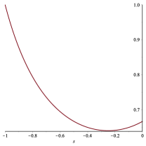
Figure 3. The graph of $F(s)=-\frac{4s+2}{4s^{3}+4s^{2}-5s-3}$ in the interval $(-1,0)$.

For $s\in(-1,-1/2)\cup(-1/2,0)$, we necessarily have $\gamma\in[16/25,1)$. But as $\lambda(2-\lambda)=\gamma$, it means that $\lambda\in(2/5,8/5)$. Therefore isosceles non-equilateral relative equilibria can exists only on non-geodesic circles parallel with the equator in a region bounded by two planes: one at distance $\frac{3}{5}\kappa^{-1/2}$ above the plane of the equator and the other at the same distance below the plane of the equator. Since $F(0)=2/3$ (see Figure 3), for $\gamma\in(16/25,2/3)$ there are two values of $s$ that satisfy the equation $\gamma=F(s)$. They correspond to values of $\lambda$ that satisfy the inequalities $16/25<\lambda(2-\lambda)<2/3,$ which translate into $\lambda\in(2/5,1-\sqrt{3}/3)\cup(1+\sqrt{3}/3,8/5)$. This means that there are two open regions, symmetrically placed relative to the equator, in which for every admissible $m$ and $M$ we find two distinct isosceles triangles that form relative equilibria. These regions are distanced at $\frac{3}{5}\kappa^{-1/2}$ (upper bound) and $\frac{\sqrt{3}}{3}\kappa^{-1/2}$ (lower bound) from the plane of the equator. When $\gamma=2/3$, there are two values of $s$ that correspond to it (see Figure 3), one of which is 0, and implies that $\cos a=0$, a case that leads to a right isosceles triangle (which cannot be a relative equilibrium since the triangle is not acute). When $\gamma=1$, only the value $s=-1$ corresponds to it, which means that $\cos a=-1$, so we have a degenerate isosceles triangle with a collision-antipodal singularity (collision between $m_{2}$ and $m_{3}$ and antipodal configuration between $m_{1}$ and the pair $m_{2}m_{3}$). Therefore this case leads to no new solutions, a remark that completes the proof. ∎

Remark 2.

In a previous paper, [4], we stated a result according to which there are no relative equilibria given by scalene triangles on parallel circles outside the equator of $\mathbb{S}_{\kappa}^{2}$. But in the mean time we found an error in the proof (we wrongly assumed that a certain relation can generate two similar relations by circular permutations). The result in [4] remains true as stated (and we will provide a correct demonstration in a future paper), in the sense of purely scalene triangular relative equilibria, i.e. with the exclusion of the isosceles relative equilibria whose existence is proved above.

6. Elliptic relative equilibria in $\mathbb{H}_{\kappa}^{2}$

In this section we study the existence of relative equilibria in $\mathbb{H}_{\kappa}^{2}$. It turns out that the set of solutions of this kind is not as rich as in $\mathbb{S}_{\kappa}^{2}$, a first manifestation of the phenomenon we mentioned earlier. More precisely we will prove the following result.

Theorem 4.

There are no isosceles relative equilibria parallel with the $xy$-plane in $\mathbb{H}_{\kappa}^{2}$, except for the Lagrangian (equilateral) solutions of equal masses, which occur on any circle parallel with the $xy$-plane.

Proof.

We start by rewriting system (1) in a convenient way, which will allow us to use part of the proof of Theorem 3 for our current purposes. For this, let us denote

$$\Psi_{i}=|\kappa|^{-1/2}\omega_{i}(|\kappa|^{1/2}\omega_{i}+2),\ \ \omega_{i}\in[0,\infty),\ \ \kappa<0,$$

and consider the change of coordinates

$$x_{i}=\Psi_{i}^{1/2}\cos\varphi_{i},\ \ y_{i}=\Psi_{i}^{1/2}\sin\varphi_{i},\ \ i=1,2,3.$$

Then some straightforward computations show that the equations of motion (1) take the form

(14) $$\begin{cases}\ddot{\varphi}_{i}=\Psi_{i}^{-1/2}\sum_{\stackrel{{\scriptstyle j=1}}{{j\neq i}}}^{3}\frac{m_{j}\Psi_{j}^{1/2}\sin(\varphi_{j}-\varphi_{i})}{\rho_{ij}^{3}\big{(}1-\frac{\kappa\rho_{ij}^{2}}{4}\big{)}^{3/2}}-\frac{\dot{\varphi}_{i}\dot{\Psi}_{i}}{\Psi_{i}}\cr\ddot{\omega}_{i}=\sum_{\stackrel{{\scriptstyle j=1}}{{j\neq i}}}^{3}\frac{m_{j}\big{[}\omega_{j}-\omega_{i}+\frac{\kappa\rho_{ij}^{2}}{2}(\omega_{i}+|\kappa|^{-1/2})\big{]}}{\rho_{ij}^{3}\big{(}1-\frac{\kappa\rho_{ij}^{2}}{4}\big{)}^{3/2}}-(\kappa\omega_{i}-|\kappa|^{\frac{1}{2}})\big{(}\frac{\dot{\Psi}_{i}^{2}}{4\Psi_{i}}+\dot{\varphi}_{i}^{2}\Psi_{i}-\dot{\omega}_{i}^{2}\big{)},\end{cases}$$

$i=1,2,3$, where

$$\dot{\Psi}_{i}=2|\kappa|^{-1/2}\dot{\omega}_{i}(|\kappa|^{1/2}\omega_{i}+1),\ \ \omega_{i}\in(0,\infty),\ \ i=1,2,3,$$

$$\rho_{ij}^{2}=\Psi_{i}+\Psi_{j}-2\Psi_{i}^{1/2}\Psi_{j}^{1/2}\cos(\varphi_{i}-\varphi_{j})-(\omega_{i}-\omega_{j})^{2},\ i,j=1,2,3,\ i\neq j.$$

Since we assume that the motion takes place in a plane parallel with the $xy$-plane on $\mathbb{H}_{\kappa}^{2}$, we can take

$$\omega_{i}=v>0,\ \ i=1,2,3.$$

The rest of the proof is identical with that for Theorem 3, with one exception: if we denote

$$\mu=|\kappa|^{1/2}v>0,\ \ \delta=-|\kappa|v(2|\kappa|^{-1/2}+v),$$

then $\gamma$ in the proof of Theorem 3 must be replaced by $\delta$ and the discussion of the inequalities related to the quadratic equation $\lambda(2-\lambda)=\gamma$ must be replaced by that of the quadratic equation in $\mu$,

$$-\mu(\mu+2)=\delta.$$

But then, in the equation $\delta=F(s)$, the only solutions occur when $F(s)=0/0$, since otherwise $\delta$ is negative and $F(s)$ positive. Like in the case of the spheres $\mathbb{S}_{\kappa}^{2}$, those solutions correspond to the Lagrangian (equilateral) triangles, a remark that completes the proof. ∎

7. Equivalent equations of motion

In this section we will obtain another form of the equations of motion that will be suitable for the study of Lagrangian relative equilibria. Let us notice first that system (1) is not analytic in $\kappa$ at $\kappa=0$ due to the occurrence of the terms $|\kappa|^{1/2}$ in the last equation. In [8], this inconvenience was solved by applying the substitution $\delta=\sigma|\kappa|^{1/2},$ and further using the parameter $\delta$ instead of $\kappa$. Here we will proceed differently. The idea, which Carles Simó kindly suggested, is to express the variables $\omega_{1},\omega_{2},\omega_{3}$ in terms of the other variables in a suitable way with the help of the constraints, such that system (1) becomes analytic for all values of $\kappa\in\mathbb{R}$. For this, we will write the constraints (2) as

$$\kappa(x_{i}^{2}+y_{i}^{2}+z_{i}^{2})+(|\kappa|^{1/2}\omega_{i}+1)^{2}=1,\ \ i=1,2,3,$$

which we solve for $\omega_{i}$ explicitly and obtain

(15) $$\omega_{i}=|\kappa|^{-1/2}\Big{[}\sqrt{1-\kappa(x_{i}^{2}+y_{i}^{2}+z_{i}^{2})}-1\Big{]},\ \ i=1,2,3.$$

We can now completely eliminate the three equations involving $\omega_{1},\omega_{2},\omega_{3}$, but these variables still occur in the terms $r_{ij}^{2}$, which show up in the other equations. Actually these variables appear in the particular form $\sigma(\omega_{i}-\omega_{j})^{2},$ which using (15) can be written as

(16) $$\sigma(\omega_{i}-\omega_{j})^{2}=\frac{\kappa(x_{i}^{2}+y_{i}^{2}+z_{i}^{2}-x_{j}^{2}-y_{j}^{2}-z_{j}^{2})^{2}}{\Big{[}\sqrt{1-\kappa(x_{i}^{2}+y_{i}^{2}+z_{i}^{2})}+\sqrt{1-\kappa(x_{j}^{2}+y_{j}^{2}+z_{j}^{2})}\ \Big{]}^{2}}.$$

For $\kappa>0$ and sufficiently small, the expressions involving square roots always exist, an assumption we will further impose in the rest of the paper. So system (1) is now reduced to the first $18$ equations without any constraints and is analytic in $\kappa$ for all small values of this parameter. In fact, as we mentioned earlier, from the physical point of view these values are the only interesting ones because should our universe be non-flat, it would for sure have a curvature that is close to zero, whether positive or negative.

Using equations (1), as well as formulas (15) and (16) with $z_{1}=z_{2}=z_{3}=0$, some differentiation leads us to the system

(17) $$\begin{cases}\ddot{x}_{i}=\sum_{j=1,j\neq i}^{3}\cfrac{m_{j}\Big{[}x_{j}-\Big{(}1-\frac{\kappa\rho_{ij}^{2}}{2}\Big{)}x_{i}\Big{]}}{\rho_{ij}^{3}\Big{(}1-\frac{\kappa\rho_{ij}^{2}}{4}\Big{)}^{3/2}}-\kappa(\dot{x}_{i}^{2}+\dot{y}_{i}^{2}+\kappa B_{i})x_{i}\cr\ddot{y}_{i}=\sum_{j=1,j\neq i}^{3}\cfrac{m_{j}\Big{[}y_{j}-\Big{(}1-\frac{\kappa\rho_{ij}^{2}}{2}\Big{)}y_{i}\Big{]}}{\rho_{ij}^{3}\Big{(}1-\frac{\kappa\rho_{ij}^{2}}{4}\Big{)}^{3/2}}-\kappa(\dot{x}_{i}^{2}+\dot{y}_{i}^{2}+\kappa B_{i})y_{i},\cr\end{cases}$$

$i=1,2,3$, where, for $i,j\in\{1,2,3\},\ i\neq j,$

(18) $$\rho_{ij}^{2}=(x_{i}-x_{j})^{2}+(y_{i}-y_{j})^{2}+\frac{\kappa(A_{i}-A_{j})^{2}}{\big{(}\sqrt{1-\kappa A_{i}}+\sqrt{1-\kappa A_{j}}\ \!\big{)}^{2}},$$

(19) $$A_{i}=x_{i}^{2}+y_{i}^{2},\ \ i=1,2,3,$$

(20) $$B_{i}=\frac{(x_{i}\dot{x}_{i}+y_{i}\dot{y}_{i})^{2}}{1-\kappa A_{i}},\ \ i=1,2,3.$$

This is the system we will further study here. Notice that for $\kappa=0$ we recover the classical Newtonian equations of the planar 3-body problem,

(21) $$\begin{cases}\ddot{x}_{i}=\sum_{j=1,j\neq i}^{3}\frac{m_{j}(x_{j}-x_{i})}{\rho_{ij}^{3}}\cr\ddot{y}_{i}=\sum_{j=1,j\neq i}^{3}\frac{m_{j}(y_{j}-y_{i})}{\rho_{ij}^{3}},\ \ i=1,2,3.\cr\end{cases}$$

For all $\kappa\in\mathbb{R}$, system (17) possesses the integral of energy,

(22) $$T_{\kappa}({\bf q},\dot{\bf q})-U_{\kappa}({\bf q})=h,$$

where $h$ is an integration constant, $T_{\kappa}$ is the kinetic energy,

(23) $$T_{\kappa}({\bf q},\dot{\bf q})=\frac{1}{2}\sum_{i=1}^{3}m_{i}(\dot{x}_{i}^{2}+\dot{y}_{i}^{2}+\kappa B_{i}),$$

and $U_{\kappa}$ is the force function,

(24) $$U_{\kappa}({\bf q})=\sum_{1\leq i<j\leq 3}\frac{m_{i}m_{j}\Big{(}1-\frac{\kappa\rho_{ij}^{2}}{2}\Big{)}}{\rho_{ij}\Big{(}1-\frac{\kappa\rho_{ij}^{2}}{4}\Big{)}^{1/2}},$$

with

$${\bf q}=({\bf q}_{1},{\bf q}_{2},{\bf q}_{3}),\ {\bf q}_{i}=(x_{i},y_{i}),\ i=1,2,3.$$

Notice that for $\kappa=0$ we recover the well-known expression of the kinetic energy,

$$T({\bf q},\dot{\bf q})=\frac{1}{2}\sum_{i=1}^{3}m_{i}(\dot{x}_{i}^{2}+\dot{y}_{i}^{2}),$$

and the force function,

$$U({\bf q})=\sum_{i=1}^{3}\frac{m_{i}m_{j}}{\rho_{ij}}.$$

To write the integrals of the total angular momentum, notice first that from (15) we have that

$$\dot{\omega}_{i}=-\sigma|\kappa|^{1/2}B_{i}^{1/2},\ \ i=1,2,3,$$

and by multiplying with the conjugate in (15), we can write that

$$\omega_{i}=-\frac{\sigma|\kappa|^{1/2}A_{i}}{1+\sqrt{1-\kappa A_{i}}},\ \ i=1,2,3.$$

Using these expressions, we can now write the three integrals of the total angular momentum,

(25) $$\sigma|\kappa|^{1/2}\sum_{i=1}^{3}m_{i}\bigg{(}B_{i}^{1/2}x_{i}-\frac{A_{i}\dot{x}_{i}}{1+\sqrt{1-\kappa A_{i}}}\bigg{)}-|\kappa|^{-1/2}\sum_{i=1}^{3}m_{i}\dot{x}_{i}=c_{1},$$

(26) $$\sigma|\kappa|^{1/2}\sum_{i=1}^{3}m_{i}\bigg{(}B_{i}^{1/2}{y}_{i}-\frac{A_{i}\dot{y}_{i}}{1+\sqrt{1-\kappa A_{i}}}\bigg{)}-|\kappa|^{-1/2}\sum_{i=1}^{3}m_{i}\dot{y}_{i}=c_{2},$$

(27) $$\sum_{i=1}^{3}\sigma m_{i}(y_{i}\dot{x}_{i}-x_{i}\dot{y}_{i})=c_{3},$$

where $c_{1},c_{2},c_{3}$ are integration constants. Notice that if we multiply equations (25) and (26) by $|\kappa|^{1/2}$, then for $\kappa=0$ these two integrals of the angular momentum become the two integrals of the linear momentum, so we are left only with one integral of the total angular momentum, equation (27), as expected to happen in the planar Euclidean case.

So for $\kappa=0$, we can write the integrals of the centre of mass and linear momentum as

(28) $$\begin{cases}\sum_{i=1}^{3}m_{i}x_{i}=0,\cr\sum_{i=1}^{3}m_{i}y_{i}=0,\cr\sum_{i=1}^{3}m_{i}\dot{x}_{i}=0,\cr\sum_{i=1}^{3}m_{i}\dot{y}_{i}=0.\cr\end{cases}$$

No such integrals, however, occur for $\kappa\neq 0$, as shown in [8].

8. The case of two negligible masses

In this section we consider the simple case when $m_{1}=:m>0$ and $m_{2}=m_{3}=0$, also known as a planetary problem. For the classical Newtonian equations, the Lagrangian relative equilibria have a particular form under such circumstances: $m_{1}$ is at rest at the origin of the coordinate system, while $m_{2}$ and $m_{3}$ move along the same circle, such that the three particles form an equilateral triangle for all time. We will further show that similar orbits exist for $\kappa\neq 0$. More precisely, we will prove the following result.

Theorem 5.

In the case of two negligible masses, there occur no bifurcations of the Lagrangian equilateral relative equilibria when passing from $\mathbb{S}_{\kappa}^{2}$ to $\mathbb{R}^{2}$ to $\mathbb{H}_{\kappa}^{2}$, as $\kappa$ goes from $+\infty$ to $-\infty$.

Proof.

Since $m_{2}=m_{3}=0$, these particles do not influence the motion of $m_{1}$. Therefore if we initially take $x_{1}(0)=y_{1}(0)=0$, the coordinates of $m_{1}$ remain the same all along the motion. Then the equations in (17) corresponding to $x_{1}$ and $y_{1}$ are identically satisfied and system (17), which now describes only the motion of $m_{2}$ and $m_{3}$, takes the form

(29) $$\begin{cases}\ddot{x}_{2}=\frac{m\big{(}\frac{\kappa\rho_{12}^{2}}{2}-1\big{)}x_{2}}{\rho_{12}^{3}\big{(}1-\frac{\kappa\rho_{12}^{2}}{4}\big{)}^{3/2}}-\kappa(\dot{x}_{2}^{2}+\dot{y}_{2}^{2}+\kappa B_{2})x_{2}\cr\ddot{y}_{2}=\frac{m\big{(}\frac{\kappa\rho_{12}^{2}}{2}-1\big{)}y_{2}}{\rho_{12}^{3}\big{(}1-\frac{\kappa\rho_{12}^{2}}{4}\big{)}^{3/2}}-\kappa(\dot{x}_{2}^{2}+\dot{y}_{2}^{2}+\kappa B_{2})y_{2}\cr\ddot{x}_{3}=\frac{m\big{(}\frac{\kappa\rho_{13}^{2}}{2}-1\big{)}x_{3}}{\rho_{13}^{3}\big{(}1-\frac{\kappa\rho_{13}^{2}}{4}\big{)}^{3/2}}-\kappa(\dot{x}_{3}^{2}+\dot{y}_{3}^{2}+\kappa B_{2})x_{3}\cr\ddot{y}_{3}=\frac{m\big{(}\frac{\kappa\rho_{13}^{2}}{2}-1\big{)}y_{3}}{\rho_{13}^{3}\big{(}1-\frac{\kappa\rho_{13}^{2}}{4}\big{)}^{3/2}}-\kappa(\dot{x}_{3}^{2}+\dot{y}_{3}^{2}+\kappa B_{2})y_{3},\cr\end{cases}$$

where

$$\rho_{12}^{2}=x_{2}^{2}+y_{2}^{2}+\frac{\kappa(x_{2}^{2}+y_{2}^{2})^{2}}{\big{[}1+\sqrt{1-\kappa(x_{2}^{2}+y_{2}^{2})}\big{]}^{2}},$$

$$\rho_{13}^{2}=x_{3}^{2}+y_{3}^{2}+\frac{\kappa(x_{3}^{2}+y_{3}^{2})^{2}}{\big{[}1+\sqrt{1-\kappa(x_{3}^{2}+y_{3}^{2})}\big{]}^{2}},$$

$$B_{2}=\frac{(x_{2}\dot{x}_{2}+y_{2}\dot{y}_{2})^{2}}{1-\kappa(x_{2}^{2}+y_{2}^{2})},\ \ \ B_{3}=\frac{(x_{3}\dot{x}_{3}+y_{3}\dot{y}_{3})^{2}}{1-\kappa(x_{3}^{2}+y_{3}^{2})}.$$

We can now show that system (29) has a solution of the form

(30) $$x_{2}=r\cos\alpha t,\ \ y_{2}=r\sin\alpha t,\ \ x_{3}=r\cos(\alpha t+\theta),\ \ y_{3}=r\sin(\alpha t+\theta),$$

where $\theta\in(0,\pi)$. This means that $m_{2}$ and $m_{3}$ move along a circle of radius $r$ on the 2-sphere or the hyperbolic 2-sphere of curvature $\kappa$, such that they form an equilateral triangle with $m_{1}$ at all times. In the 3-dimensional flat ambient space, the particles form an equilateral triangle that is not parallel with the $xy$-plane. The projection of the $2\pi/3$-angle between the sides $m_{1}m_{2}$ and $m_{1}m_{3}$ on the $xy$-plane is $\theta$, an angle that depends on $r$. The projection of the other two angles of the equilateral triangle onto the $xy$-plane is also different from $2\pi/3$.

To show that (30) is a solution of system (29), notice first that

$$\rho^{2}:=\rho_{12}^{2}=\rho_{13}^{2}=\frac{2r^{2}}{1+\sqrt{1-\kappa r^{2}}},\ \ \ B_{2}=B_{3}=0.$$

But the point masses $m_{1},m_{2},m_{3}$ form an equilateral triangle only if the condition

$$\rho^{2}=\rho_{23}^{2}=2(1-\cos\theta)r^{2}$$

is also satisfied. This condition leads to the connection between $\theta$ and $r$, namely

$$\cos\theta=\frac{\sqrt{1-\kappa r^{2}}}{1+\sqrt{1-\kappa r^{2}}}.$$

Then some straightforward computations prove that all four equations in system (29) lead to the same relationship,

(31) $$\alpha^{2}=\frac{m(1-\kappa r^{2}+\sqrt{1-\kappa r^{2}})}{r^{3}(1-\kappa r^{2})(1+\sqrt{1-\kappa r^{2}})},$$

which shows how the angular velocity $\alpha$ of the particles $m_{2}$ and $m_{3}$ depends on the constants $\kappa,m$, and $r$. Since for $\kappa,m$, and $r$ fixed there are always two values of $\alpha$ that satisfy the above relationship, one corresponding to each direction of rotation, it means that Lagrangian relative equilibria of this kind exist. ∎

9. The case of one negligible mass

We further consider the case when $m_{1}=:M>0,m_{2}=:m>0$ and $m_{3}=0$. For the classical Newtonian equations, the Lagrangian relative equilibria have a particular form under such circumstances: $m_{1}$ and $m_{2}$ lie on a straight line that rotates around the centre of mass of these particles, each moving along a circle, while $m_{3}$ moves on another circle, concentric with the other two, such that all three particles form an equilateral triangle at all times. We will further find out what happens for $\kappa\neq 0$.

Since $m_{3}=0$, this particle does not influence the motion of $m_{1}$ and $m_{2}$. System (17) thus takes the form

(32) $$\begin{cases}\ddot{x}_{1}=\frac{m\Big{[}x_{2}-\Big{(}1-\frac{\kappa\rho_{12}^{2}}{2}\Big{)}x_{1}\Big{]}}{\rho_{12}^{3}\Big{(}1-\frac{\kappa\rho_{12}^{2}}{4}\Big{)}^{3/2}}-\kappa(\dot{x}_{1}^{2}+\dot{y}_{1}^{2}+\kappa B_{1})x_{1}\cr\ddot{y}_{1}=\frac{m\Big{[}y_{2}-\Big{(}1-\frac{\kappa\rho_{12}^{2}}{2}\Big{)}y_{1}\Big{]}}{\rho_{12}^{3}\Big{(}1-\frac{\kappa\rho_{12}^{2}}{4}\Big{)}^{3/2}}-\kappa(\dot{x}_{1}^{2}+\dot{y}_{1}^{2}+\kappa B_{1})y_{1}\cr\ddot{x}_{2}=\frac{M\Big{[}x_{1}-\Big{(}1-\frac{\kappa\rho_{12}^{2}}{2}\Big{)}x_{2}\Big{]}}{\rho_{12}^{3}\Big{(}1-\frac{\kappa\rho_{12}^{2}}{4}\Big{)}^{3/2}}-\kappa(\dot{x}_{2}^{2}+\dot{y}_{2}^{2}+\kappa B_{2})x_{2}\cr\ddot{y}_{2}=\frac{M\Big{[}y_{1}-\Big{(}1-\frac{\kappa\rho_{12}^{2}}{2}\Big{)}y_{2}\Big{]}}{\rho_{12}^{3}\Big{(}1-\frac{\kappa\rho_{12}^{2}}{4}\Big{)}^{3/2}}-\kappa(\dot{x}_{2}^{2}+\dot{y}_{2}^{2}+\kappa B_{2})y_{2}\cr\ddot{x}_{3}=\frac{M\Big{[}x_{1}-\Big{(}1-\frac{\kappa\rho_{13}^{2}}{2}\Big{)}x_{3}\Big{]}}{\rho_{13}^{3}\Big{(}1-\frac{\kappa\rho_{13}^{2}}{4}\Big{)}^{3/2}}+\frac{m\Big{[}x_{2}-\Big{(}1-\frac{\kappa\rho_{23}^{2}}{2}\Big{)}x_{3}\Big{]}}{\rho_{23}^{3}\Big{(}1-\frac{\kappa\rho_{23}^{2}}{4}\Big{)}^{3/2}}-\kappa(\dot{x}_{3}^{2}+\dot{y}_{3}^{2}+\kappa B_{3})x_{3}\cr\ddot{y}_{3}=\frac{M\Big{[}y_{1}-\Big{(}1-\frac{\kappa\rho_{13}^{2}}{2}\Big{)}y_{3}\Big{]}}{\rho_{13}^{3}\Big{(}1-\frac{\kappa\rho_{13}^{2}}{4}\Big{)}^{3/2}}+\frac{m\Big{[}y_{2}-\Big{(}1-\frac{\kappa\rho_{23}^{2}}{2}\Big{)}y_{3}\Big{]}}{\rho_{23}^{3}\Big{(}1-\frac{\kappa\rho_{23}^{2}}{4}\Big{)}^{3/2}}-\kappa(\dot{x}_{3}^{2}+\dot{y}_{3}^{2}+\kappa B_{3})y_{3},\cr\end{cases}$$

which is decoupled, since the first four equations are independent of the last two equations. Here we have denoted by

$$\rho_{12}^{2}=(x_{1}-x_{2})^{2}+(y_{1}-y_{2})^{2}+\frac{\kappa(x_{1}^{2}+y_{1}^{2}-x_{2}^{2}-y_{2}^{2})^{2}}{\big{[}\sqrt{1-\kappa(x_{1}^{2}+y_{1}^{2})}+\sqrt{1-\kappa(x_{2}^{2}+y_{2}^{2})}\big{]}^{2}},$$

$$\rho_{13}^{2}=(x_{1}-x_{3})^{2}+(y_{1}-y_{3})^{2}+\frac{\kappa(x_{1}^{2}+y_{1}^{2}-x_{3}^{2}-y_{3}^{2})^{2}}{\big{[}\sqrt{1-\kappa(x_{1}^{2}+y_{1}^{2})}+\sqrt{1-\kappa(x_{3}^{2}+y_{3}^{2})}\big{]}^{2}},$$

$$\rho_{23}^{2}=(x_{2}-x_{3})^{2}+(y_{2}-y_{3})^{2}+\frac{\kappa(x_{2}^{2}+y_{2}^{2}-x_{3}^{2}-y_{3}^{2})^{2}}{\big{[}\sqrt{1-\kappa(x_{2}^{2}+y_{2}^{2})}+\sqrt{1-\kappa(x_{3}^{2}+y_{3}^{2})}\big{]}^{2}},$$

$$B_{1}=\frac{(x_{1}\dot{x}_{1}+y_{1}\dot{y}_{1})^{2}}{1-\kappa(x_{1}^{2}+y_{1}^{2})},\ \ \ B_{2}=\frac{(x_{2}\dot{x}_{2}+y_{2}\dot{y}_{2})^{2}}{1-\kappa(x_{2}^{2}+y_{2}^{2})},\ \ \ B_{3}=\frac{(x_{3}\dot{x}_{3}+y_{3}\dot{y}_{3})^{2}}{1-\kappa(x_{3}^{2}+y_{3}^{2})}.$$

In the flat case, $m_{1}$ and $m_{2}$ lie on an axis that rotates around the centre of mass of these particles. Thus $m_{1}$ and $m_{2}$ move, in general, on concentric circles; if $m_{1}=m_{2}$, they move on the same circle. The particle $m_{3}$ forms all the time an equilateral triangle with $m_{1}$ and $m_{2}$ and moves on a circle that is concentric with the other (one or two) circles.

We will therefore place $m_{1}$ and $m_{2}$ on a geodesic passing through and rotating around the contact point of $\mathbb{S}_{\kappa}^{2},\mathbb{R}^{2}$, and $\mathbb{H}_{\kappa}^{2}$ (see Figure 1). Then, if a Lagrangian orbit exists, $m_{3}$ must move on a circle of $\mathbb{S}_{\kappa}^{2}$ or $\mathbb{H}_{\kappa}^{2}$. So if we take a fixed angle $\theta\in(0,\pi)$, we are seeking a solution of the form

(33) $$x_{1} =r_{1}\cos\alpha t,\ \ \ \ \ \ \ \ \ \ y_{1}=r_{1}\sin\alpha t$$

(34) $$x_{2} =-r_{2}\cos\alpha t,\ \ \ \ \ \ \ \ \!y_{2}=-r_{2}\sin\alpha t$$

(35) $$x_{3} =r_{3}\cos(\alpha t+\theta),\ \ \ y_{3}=r_{3}\sin(\alpha t+\theta),$$

with $r_{1},r_{2},r_{3}>0$ and, in the case of $\mathbb{S}_{\kappa}^{2}$, no larger than the radius of the sphere. Then it follows that for this candidate solution we have

(36) $$B_{1}=B_{2}=B_{3}=0,$$

(37) $$\rho_{12}^{2}=(r_{1}+r_{2})^{2}+\frac{\kappa(r_{1}^{2}-r_{2}^{2})^{2}}{(\sqrt{1-\kappa r_{1}^{2}}+\sqrt{1-\kappa r_{2}^{2}})^{2}},$$

(38) $$\rho_{13}^{2}=r_{1}^{2}+r_{2}^{2}+2r_{1}r_{2}\cos\theta+\frac{\kappa(r_{1}^{2}-r_{3}^{2})^{2}}{(\sqrt{1-\kappa r_{1}^{2}}+\sqrt{1-\kappa r_{3}^{2}})^{2}},$$

(39) $$\rho_{23}^{2}=r_{2}^{2}+r_{3}^{2}+2r_{2}r_{3}\cos\theta+\frac{\kappa(r_{2}^{2}-r_{3}^{2})^{2}}{(\sqrt{1-\kappa r_{2}^{2}}+\sqrt{1-\kappa r_{3}^{2}})^{2}}.$$

Since the triangle is equilateral, we must have

(40) $$\rho_{12}=\rho_{13}=\rho_{23}=:\rho.$$

Substituting (33) and (34) in the first and third as well as in the second and fourth equations of system (32), we can respectively conclude that

(41) $$\alpha^{2}r_{1}(1-\kappa r_{1}^{2})=\frac{m\big{(}r_{1}+r_{2}-\frac{\kappa\rho^{2}r_{1}}{2}\big{)}}{\rho^{3}\big{(}1-\frac{\kappa\rho^{2}}{4}\big{)}^{3/2}},$$

(42) $$\alpha^{2}r_{2}(1-\kappa r_{2}^{2})=\frac{M\big{(}r_{1}+r_{2}-\frac{\kappa\rho^{2}r_{2}}{2}\big{)}}{\rho^{3}\big{(}1-\frac{\kappa\rho^{2}}{4}\big{)}^{3/2}},$$

relationships which imply that the Lagrangian solution of the decoupled system given by the first four equations in (32) exists only if

(43) $$\frac{m\big{(}r_{1}+r_{2}-\frac{\kappa\rho^{2}r_{1}}{2}\big{)}}{r_{1}(1-\kappa r_{1}^{2})}=\frac{M\big{(}r_{1}+r_{2}-\frac{\kappa\rho^{2}r_{2}}{2}\big{)}}{r_{2}(1-\kappa r_{2}^{2})}.$$

This identity is obviously satisfied when $r_{1}=r_{2}$ and $M=m$. Let us first deal with this case.

9.1. Two equal masses and one negligible mass in $\mathbb{S}_{\kappa}^{2}$

In this subsection we will prove the following result.

Theorem 6.

Assume that two bodies of equal mass move on a non-equatorial parallel circle of the sphere $\mathbb{S}_{\kappa}^{2}$, being always diametrically opposed and form a Lagrangian relative equilibrium with a third body, which has negligible mass. Then the circle on which the two bodies move must have its radius equal to $(2\kappa)^{-1/2}$ and the third body must move on the equator. In other words, given $\kappa$, the size of the equilateral triangle does not depend on the value of the equal masses, but the angular velocity of the equilateral triangle does.

Proof.

So we assume that the motion takes place in $\mathbb{S}_{\kappa}^{2}$, that $0<r_{1}=r_{2}=:r<\kappa^{-1/2}$, $M=m$, and $m_{3}$ is negligible. Notice that $\kappa^{-1/2}=:R_{\kappa}$ is the radius of $\mathbb{S}_{\kappa}^{2}$. Also remark that in this case the geodesic passing through $m_{3}$ and the North Pole of the sphere is orthogonal to the geodesic connecting $m_{1}$ and $m_{2}$. If we project these geodesics on the $xy$-plane, the projections are also orthogonal. This implies that the angle $\theta$ taken in (35) is $\pi/2$, so the solution we are now checking is of the form

(44) $$x_{1} =r\cos\alpha t,\ \ \ \ \ \ \ \!y_{1}=r\sin\alpha t$$

(45) $$x_{2} =-r\cos\alpha t,\ \ \ \ y_{2}=-r\sin\alpha t$$

(46) $$x_{3} =-r_{3}\sin\alpha t,\ \ \ y_{3}=r_{3}\cos\alpha t.$$

From (37) and (40), we can conclude that for a solution of system (32) of the form (44)–(46) we have

$$\rho=2r.$$

This fact together with relations (38) and (39) for $\theta=\pi/2$ and with equation (40) imply on one hand that

(47) $$3r^{2}=r_{3}^{2}+\frac{\kappa(r^{2}-r_{3}^{2})^{2}}{(\sqrt{1-\kappa r^{2}}+\sqrt{1-\kappa r_{3}^{2}})^{2}}.$$

On the other hand, we have from (41) and (42) that

(48) $$\alpha^{2}(1-\kappa r^{2})=\frac{m\big{(}2-\frac{\kappa\rho^{2}}{2}\big{)}}{\rho^{3}\big{(}1-\frac{\kappa\rho^{2}}{4}\big{)}^{3/2}},$$

and from the last two equations in (32) that

(49) $$\alpha^{2}(1-\kappa r_{3}^{2})=\frac{2m\big{(}1-\frac{\kappa\rho^{2}}{2}\big{)}}{\rho^{3}\big{(}1-\frac{\kappa\rho^{2}}{4}\big{)}^{3/2}}.$$

By comparing (48) and (49) we are led to the relationship

(50) $$r_{3}=\sqrt{2}r.$$

Substituting (50) into (47), we obtain

(51) $$r=(2\kappa)^{-1/2}\ \ {\rm or}\ \ r=R_{\kappa}/\sqrt{2},$$

which also implies that $r_{3}=R_{\kappa}$. Then we also obtain that

(52) $$\alpha^{2}=2m\kappa^{3/2}\ \ {\rm or}\ \ \alpha^{2}=2m/R_{\kappa}^{3}.$$

From the geometric-dynamical point of view, the above results describe a surprising situation. Since $r_{3}=R_{\kappa}$, it means that the projection of the height from $m_{3}$ of the equilateral triangle $m_{1}m_{2}m_{3}$ onto the $xy$-plane has the same Euclidean length as the radius of the sphere. Therefore the particle $m_{3}$ must rotate on the equator that is parallel to the $xy$-plane, while the particles $m_{1}$ and $m_{2}$ rotate on a non-geodesic circle that is also parallel with the $xy$-plane. This circle has radius $r=R_{\kappa}/\sqrt{2}$, so it is uniquely determined only by the given sphere (therefore cannot be chosen arbitrarily). So, for a given sphere, the equilateral triangle has always the same size, independently of the values of the masses. But the angular velocity, $\alpha$, depends on the value, $m$, of the two equal masses and on the curvature, $\kappa>0$, or radius $R_{\kappa}$, of the sphere $\mathbb{S}_{\kappa}^{2}$. This remark completes the proof. ∎

9.2. Two equal masses and one negligible mass in $\mathbb{H}_{\kappa}^{2}$

In this subsection we will prove the following result, which shows again that the dynamics on $\mathbb{H}_{\kappa}^{2}$ is not as rich as in $\mathbb{S}_{\kappa}^{2}$.

Theorem 7.

There are no Lagrangian relative equilibria in $\mathbb{H}_{\kappa}^{2}$ with two bodies of equal mass and a third body of negligible mass.

Proof.

So assume that the motion takes place in $\mathbb{H}_{\kappa}^{2}$, that $r_{1}=r_{2}=:r>0$, $M=m$, and $m_{3}$ is negligible. In this case the imaginary radius of the hyperbolic sphere is $(-\kappa)^{-1/2}=:R_{\kappa}$. We can proceed as in the case of the sphere discussed in Subsection 9.1, and the solution we are checking has the same form, (44)–(46). The computations are then identical up to formula (50). But after substituting (50) into (47), we are led to the conclusion that

$$\frac{\kappa r^{2}}{(\sqrt{1-\kappa r^{2}}+\sqrt{1-2\kappa r^{2}})^{2}}=1,$$

which is impossible since $\kappa<0$. Therefore we must conclude that there are no Lagrangian relative equilibria of this type in $\mathbb{H}_{\kappa}^{2}$. ∎

9.3. The general case

We now return to the general case and assume, without loss of generality, that $M\geq m$. Under this hypothesis we can prove the following result.

Theorem 8.

If one of the three masses is negligible,

(i) there are no Lagrangian relative equilibria in $\mathbb{H}_{\kappa}^{2}$;

(ii) there are no Lagrangian relative equilibria in $\mathbb{S}_{\kappa}^{2}$ if the curvature $\kappa$ is sufficiently small, unless the two non-negligible masses are equal, in which case the solutions occur as stated in Theorem 6.

Proof.

If we substitute a candidate solution of the form (33)–(35) into the last two equations of system (32), we obtain equations that involve $\cos\alpha t,\sin\alpha t$, on one hand, and $\cos(\alpha t+\theta),\sin(\alpha t+\theta)$ on the other hand. Separating the arguments $\alpha t$ and $\theta\in(0,\pi)$, and arguing that the equations must be satisfied for all $t\in\mathbb{R}$, we are led to the relationships

(53) $$\alpha^{2}r_{3}(1-\kappa r_{3}^{2})=\frac{(M+m)\big{(}1-\frac{\kappa\rho^{2}}{2}\big{)}r_{3}}{\rho^{3}\big{(}1-\frac{\kappa\rho^{2}}{4}\big{)}^{3/2}},$$

(54) $$\alpha^{2}r_{3}(1-\kappa r_{3}^{2})\cos\theta=-\frac{Mr_{1}-mr_{2}}{\rho^{3}\big{(}1-\frac{\kappa\rho^{2}}{4}\big{)}^{3/2}}+\frac{(M+m)\big{(}1-\frac{\kappa\rho^{2}}{2}\big{)}r_{3}\cos\theta}{\rho^{3}\big{(}1-\frac{\kappa\rho^{2}}{4}\big{)}^{3/2}},$$

which are simultaneously satisfied only if

(55) $$Mr_{1}=mr_{2}.$$

The case of $M=m$ and $r_{1}=r_{2}$, which corresponds to $\theta=\pi/2$ and was already treated in subsections 9.1 and 9.2, is in agreement with relation (55) and its derivation from (53) and (54).

Writing (55) as $m/r_{1}=M/r_{2}$, we can conclude from (43) that

(56) $$(r_{1}-r_{2})\Big{[}\frac{\rho^{2}}{2}(1+\kappa r_{1}r_{2})-(r_{1}+r_{2})^{2}\Big{]}=0.$$

Therefore we must split our analysis into two cases.

Case 1: $r_{1}=r_{2}$. With this hypothesis it follows from (55) that $M=m$, a situation we already settled in subsections 9.1 and 9.2. Moreover, for $\kappa>0$, the relationship between $r$ and $r_{3}$ that we obtain from (43) and (53) is identical with the one we computed in subsection 9.1, so this case is completely solved.

Case 2: $\frac{\rho^{2}}{2}(1+\kappa r_{1}r_{2})-(r_{1}+r_{2})^{2}=0$. Under these circumstances we must start with the hypothesis $r_{1}\neq r_{2}$. Since we assumed $M\geq m$, relation (55) implies that we cannot have $r_{1}>r_{2}$, so the initial hypothesis leads to the conclusion that $r_{1}<r_{2}$ and, consequently, $M>m$. If we denote $r:=r_{1}$ and $\mu:=M/m\geq 1$, then $r_{2}=\mu r$ and

(57) $$\frac{\rho^{2}}{2}(1+\kappa r_{1}r_{2})-(r_{1}+r_{2})^{2}=\frac{\rho^{2}}{2}(1+\kappa\mu r^{2})-(1+\mu)^{2}r^{2}.$$

But from (37), we obtain that

(58) $$\rho^{2}=(1+\mu)^{2}r^{2}+\frac{\kappa(1-\mu)^{2}r^{4}}{(\sqrt{1-\kappa r^{2}}+\sqrt{1-\kappa\mu^{2}r^{2}})^{2}}.$$

If $\kappa<0$, we can see from (58) that

$$\rho^{2}\leq(1+\mu)^{2}r^{2}.$$

Consequently, using the above relation and (57), we have the inequality

$$\frac{\rho^{2}}{2}(1+\kappa r_{1}r_{2})-(r_{1}+r_{2})^{2}\leq\frac{1}{2}(1+\mu)^{2}r^{2}(\kappa\mu r^{2}-1).$$

But for $\kappa<0$, the right hand side of this inequality is negative, so the second factor in (56) cannot be zero. We can thus conclude from here and from the result obtained in subsection 9.2 that there are no Lagrangian relative equilibria on 2-dimensional hyperbolic spheres in the case of one negligible mass.

If $\kappa>0$ and sufficiently small, then

$$(\sqrt{1-\kappa r^{2}}+\sqrt{1-\kappa\mu^{2}r^{2}})^{2}<1.$$

From (58) we can thus draw the conclusion that

$$\rho^{2}<(1+\mu)^{2}r^{2}+\kappa(1-\mu)^{2}r^{4}.$$

Using the above relationship and (57) we obtain the inequality

(59) $$\frac{\rho^{2}}{2}(1+\kappa r_{1}r_{2})-(r_{1}+r_{2})^{2}<\frac{1}{2}[(1+\mu)^{2}r^{2}(\kappa\mu r^{2}-1)+\kappa(1-\mu)^{2}r^{4}(1+\kappa\mu r^{2})].$$

Let us further see

(60) $$\kappa\mu r^{2}-1\leq 0$$

even for large values of $\kappa>0$. For this, notice that from the second square root in the denominator of (58), we must have

$$1-\kappa\mu^{2}r^{2}\geq 0,$$

which is the same as

$$r\leq\frac{m}{M}R_{\kappa},$$

where, recall, $\kappa=1/R_{\kappa}^{2}$. But $0<m/M<1$, so the above inequality implies that

$$r\leq\sqrt{\frac{m}{M}}R_{\kappa},$$

a relationship that is equivalent to (60) and that is always satisfied.

From (60) we now obtain that for $\kappa>0$ and sufficiently small, the right hand side of (59) is negative, thus

$$\frac{\rho^{2}}{2}(1+\kappa r_{1}r_{2})-(r_{1}+r_{2})^{2}<0,$$

and consequently there are no Lagrangian relative equilibria in Case 2.

So for one negligible mass, we can conclude that Lagrangian relative equilibria do not exist for negative curvature, and that they occur for small positive curvature only if $M=m$. Since the case $|\kappa|<\!\!<1$ is the only one of relevance when studying the curvature of the large-scale universe, we will not further investigate here what happens for other positive values of $\kappa$. ∎

Acknowledgments. The author is indebted to Regina Martínez, Carles Simó, and Ernesto Pérez-Chavela for several discussions on this topic.

References

- [1] J. Bertrand, Théorème relatif au mouvement d’un point attiré vers un center fixe, C. R. Acad. Sci. 77 (1873), 849-853.
- [2] W. Bolyai and J. Bolyai, Geometrische Untersuchungen, Hrsg. P. Stäckel, Teubner, Leipzig-Berlin, 1913.
- [3] F. Diacu, On the singularities of the curved -body problem, Trans. Amer. Math. Soc. 363, 4 (2011), 2249–2264.
- [4] F. Diacu, Polygonal homographic orbits of the curved 3-body problem, Trans. Amer. Math. Soc. 364 (2012), 2783–2802.
- [5] F. Diacu, Relative equilibria of the curved -body problem, Atlantis Studies in Dynamical Systems, vol. 1, Atlantis Press, Amsterdam, 2012.
- [6] F. Diacu, Relative equilibria of the 3-dimensional curved -body problem, Memoirs Amer. Math. Soc. 228, 1071 (2013).
- [7] F. Diacu, The curved -body problem: risks and rewards, Math. Intelligencer 35, 3 (2013), 24–33.
- [8] F. Diacu, The classical -body problem in the context of curved space, arXiv:1405.0453.
- [9] F. Diacu and S. Kordlou, Rotopulsators of the curved -body problem, J. Differential Equations 255 (2013) 2709–2750.
- [10] F. Diacu, R. Martínez, E. Pérez-Chavela, and C. Simó, On the stability of tetrahedral relative equilibria in the positively curved 4-body problem, Physica D 256-7 (2013), 21-35.
- [11] F. Diacu and E. Pérez-Chavela, Homographic solutions of the curved -body problem, J. Differential Equations 250 (2011), 340–366.
- [12] F. Diacu, E. Pérez-Chavela, and M. Santoprete, Saari’s conjecture for the collinear -body problem, Trans. Amer. Math. Soc. 357, 10 (2005), 4215–4223.
- [13] F. Diacu, E. Pérez-Chavela, and M. Santoprete, The -body problem in spaces of constant curvature. Part I: Relative equilibria, J. Nonlinear Sci. 22, 2 (2012), 247–266, DOI: 10.1007/s00332-011-9116-z.
- [14] F. Diacu, E. Pérez-Chavela, and M. Santoprete, The -body problem in spaces of constant curvature. Part II: Singularities, J. Nonlinear Sci. 22, 2 (2012), 267–275, DOI: 10.1007/s00332-011-9117-y.
- [15] F. Diacu, E. Pérez-Chavela, and J. Guadalupe Reyes Victoria, An intrinsic approach in the curved -body problem. The negative curvature case, J. Differential Equations 252 (2012), 4529–4562.
- [16] F. Diacu and S. Popa, All Lagrangian relative equilibria have equal masses, J. Math. Phys. 55, 112701 (2014).
- [17] F. Diacu and B. Thorn, Rectangular orbits of the curved 4-body problem, Proc. Amer. Math. Soc. 143 (2015), 1583–1593.
- [18] L. Euler, Considerationes de motu corporum coelestium, Novi commentarii academiae scientiarum Petropolitanae 10 (1764), 1766, pp. 544Ð558 (read at Berlin in april 1762). Also in Opera Omnia, S. 2, vol. 25, pp. 246-257 with corrections and comments by M. Schürer.
- [19] L.C. García-Naranjo, J.C. Marrero, E. Pérez-Chavela, M. Rodríguez-Olmos, Classification and stability of relative equilibria for the two-body problem in the hyperbolic space of dimension 2, arXiv:1505.01452.
- [20] W. Killing, Die Rechnung in den nichteuklidischen Raumformen, J. Reine Angew. Math. 89 (1880), 265–287.
- [21] H. Kragh, Is space Flat? Nineteenth century astronomy and non-Euclidean geometry, J. Astr. Hist. Heritage 15, 3 (2012), 149-158.
- [22] J.L. Lagrange, Essai sur le problème des trois corps, 1772, Œuvres tome 6.
- [23] H. Liebmann, Die Kegelschnitte und die Planetenbewegung im nichteuklidischen Raum, Berichte Königl. Sächsischen Gesell. Wiss., Math. Phys. Klasse 54 (1902), 393-423.
- [24] H. Liebmann, Über die Zentralbewegung in der nichteuklidische Geometrie, Berichte Königl. Sächsischen Gesell. Wiss., Math. Phys. Klasse 55 (1903), 146-153.
- [25] R. Lipschitz, Extension of the planet-problem to a space of dimensions and constant integral curvature, Quart. J. Pure Appl. Math. 12 (1873), 349-370.
- [26] N. I. Lobachevsky, The new foundations of geometry with full theory of parallels [in Russian], 1835-1838, In Collected Works, V. 2, GITTL, Moscow, 1949, p. 159.
- [27] R. Martínez and C. Simó, On the stability of the Lagrangian homographic solutions in a curved three-body problem on , Discrete Contin. Dyn. Syst. Ser. A 33 (2013) 1157-1175.
- [28] R. Martínez and C. Simó, Relative equilibria of the restricted 3-body problem in curved spaces, (in preparation).
- [29] E. Pérez-Chavela and J.G. Reyes Victoria, An intrinsic approach in the curved -body problem. The positive curvature case, Trans. Amer. Math. Soc. 364, 7 (2012), 3805-3827.
- [30] B. Riemann, Über die Hypothesen welche der Geometrie zu Grunde liegen, Abhandl. Königl. Ges. Wiss. Gött., 13, 1854.
- [31] E. Schering, Die Schwerkraft im Gaussischen Räume, Nachr. Königl. Ges. Wiss. Gött. 15, (1870), 311–321.
- [32] E. Schering, Die Schwerkraft in mehrfach ausgedehnten Gaussischen und Riemmanschen Räumen. Nachr. Königl. Ges. Wiss. Gött. 6, (1873), 149–159
- [33] A.V. Shchepetilov, Nonintegrability of the two-body problem in constant curvature spaces, J. Phys. A: Math. Gen. V. 39 (2006), 5787-5806; corrected version at math.DS/0601382.
- [34] P. Tibboel, Polygonal homographic orbits in spaces of constant curvature, Proc. Amer. Math. Soc. 141 (2013), 1465–1471.
- [35] P. Tibboel, Existence of a class of rotopulsators, J. Math. Anal. Appl. 404 (2013), 185–191.
- [36] P. Tibboel, Existence of a lower bound for the distance between point masses of relative equilibria in spaces of constant curvature, J. Math. Anal. Appl. 416 (2014), 205–211.
- [37] S. Zhu, Eulerian relative equilibria of the curved 3-body problems in , Proc. Amer. Math. Soc. 142 (2014), 2837–2848.