Stochastic Model of the Spin Distribution of Dark Matter Halos

Abstract

We employ a stochastic approach to probing the origin of the log-normal distributions of halo spin in N-body simulations. After analyzing spin evolution in halo merging trees, it was found that a spin change can be characterized by a stochastic random walk of angular momentum. Also, spin distributions generated by random walks are fairly consistent with those directly obtained from N-body simulations. We derived a stochastic differential equation from a widely used spin definition and measured the probability distributions of the derived angular momentum change from a massive set of halo merging trees. The roles of major merging and accretion are also statistically analyzed in evolving spin distributions. Several factors (local environment, halo mass, merging mass ratio, and redshift) are found to influence the angular momentum change. The spin distributions generated in the mean-field or void regions tend to shift slightly to a higher spin value compared with simulated spin distributions, which seems to be caused by the correlated random walks. We verified the assumption of randomness in the angular momentum change observed in the N-body simulation and detected several degrees of correlation between walks, which may provide a clue for the discrepancies between the simulated and generated spin distributions in the voids. However, the generated spin distributions in the group and cluster regions successfully match the simulated spin distribution. We also demonstrated that the log-normality of the spin distribution is a natural consequence of the stochastic differential equation of the halo spin, which is well described by the Geometric Brownian Motion model.

1. Introduction

Primordial angular momentum is believed to decay with the expansion of the universe and the observed rotations of galaxies and clusters are believed to originate from tidal interactions with local environments (the tidal torque theory) or the acquisition of orbital angular momentum from infalling matter (the merging theory). In the tidal torque theory (Hoyle, 1949; Peebles, 1969; Lee & Pen, 2001; Prociani et al., 2002; Lee & Erdogdu, 2007), a collapsing cloud at the turn-around epoch may obtain a tidal torque due to the misalignment between the local tidal shear and structural inertia tensor. Consequently, the spin directions of halos may provide information on the nearby mass distribution (Aragon-Calvo & Yang, 2014; Zhang et al., 2009; Trowland et al., 2013), although some studies (Lee & Erdogdu, 2007; Varela et al., 2012) have reported inconclusive or opposing results from observations. On the other hand, the merging theory (Gardner, 2001; Vitvitska et al., 2002; Maller et al., 2002) focuses on the change in angular momentum in hierarchical clusterings through the off-center infall of nearby objects/matter to drive the sudden change in halo spin (Bett & Frenk, 2012). However, D’Onghia & Navarro (2007) argued that simulated halos do not show any obvious correlation between spin and merger history.

Each theory views the same object from different angles. A dark matter halo is not static but dynamically evolves through the sometimes violent, sometimes quiet ingestion of nearby matter. According to hierarchical clustering (Cole & lacey, 1996; Jiang et al., 2014), large halos grow in mass by assimilating nearby smaller halos. However, a small satellite halo tends to have a spiral infall motion with a finite orbital angular momentum around the central halo, which, after merging, causes a net change in rotational angular momentum of the merging remnants. This non-radial infall motion of satellites may be derived from the tidal torque of anisotropic matter distributions around the central halo. However, the acquisition of satellite orbital angular momentum described in the merging theory is analogous to that of a mass shell in the tidal torque theory because they are based on the same ground: the tidal torque generated by local environments. The only difference is whether they consider the infalling source to be a satellite or a mass shell. By extending the original tidal torque theory of a spherical collapse to the multiple-shell collapses at different epochs, the tension between the two theories may be relaxed.

The distributions of halo spin have been reported to be well fitted by the log-normal function (Gardner, 2001; Bailin & Steinmetz, 2005; Bullock et al., 2001; Muñoz-Cuartas et al., 2011), with small deviations depending on the definition of the halo samples (Bett et al., 2007; Knebe & Power, 2008; Antonuccio-Delogu et al., 2010). Researchers have found that massive cluster halos are not yet relaxed from recent mergers and are responsible for the over-population of the high-$\lambda$ tail compared to the log-normal distribution (Bett et al., 2007; Hahn et al., 2007).

Antonuccio-Delogu et al. (2010) explored the origin of the log-normality of spin distributions based on the stochastic variables of halo angular momentum ($\boldsymbol{J}$), total energy ($E$), and mass ($M$). Theirs was the first attempt of its kind to address this issue. They introduced stochasticity between the two terms ${|\boldsymbol{J}|}/M^{5/2}$ and $E$ and argued that deviations from the log-normal functional form are mainly due to correlations between the two terms. However, they did not provide a physical or probable reason for the stochasticity between the two terms.

In the present study, we analyze the origin of the halo spin distribution. Using simulated mass histories of individual halos and the stochastic differential equation of the angular momentum change, we model the spin evolution using the stochastic model, distinguishing between the roles of major merging and accretion in shaping the spin distributions in various situations (Hetznecker & Burkert, 2006; Antonuccio-Delogu et al., 2002; Gardner, 2001; Lemson & Kauffmann, 1999).

This paper is organized as follows. In section 2, we describe the stochastic for spin evolution. Then, in section 3, we describe the simulation data, merging trees, and local environments of a halo. From the simulated merging history, we measure distributions of angular momentum change with respect to halo mass, spin, local environments, infall mass ratio, and redshift in section 4. In section 5, using the simulated mass histories of individual halos, we randomly generate spin changes and compare the spin distributions of the stochastic model and $N$-body simulations. In section 6, we verify how a random-walk process produces the log-normal distribution of the halo spin. We summarize the results of our study in section 7

All of the logarithms used in the equations and figures in this study are base 10.

2. Analytic Descriptions

2.1. Definition of Spins

Peebles (1969) first proposed a dimensionless parameter to quantify the rotation of a cosmic object or halo as

$$\lambda={{\sqrt{E}|\boldsymbol{J}|}\over{GM^{5/2}}},$$ (1)

where $\lambda$ is the spin, $E$ is the total energy, $M$ is the virial mass, and $\boldsymbol{J}$ is the rotational angular momentum of a halo. However, measuring halo potential is practically bothersome, and the potential of an open system is sometimes ill-defined. Therefore, another definition was proposed by Bullock et al. (2001), which reads as

$$\lambda^{\prime}_{o}={{|\bf{J}|}\over\sqrt{2}MRV},$$ (2)

where $R$ is the virial radius, and $V$ is the virial circular velocity. The virial radius can be derived from the definition of virial mass as

$$M={4\pi\over 3}R^{3}\rho_{c}(z)\Delta_{\rm vir}(z),$$ (3)

where $\rho_{c}$ is the critical density at redshift $z$, $\Delta_{\rm vir}\simeq(18\pi^{2}+82x-39x^{2})$, and $x\equiv\Omega(z)-1$ for a flat universe (Bryan & Norman, 1998). These widely used spin parameters are equivalent to $\lambda$ in the case of an idealized halo; halos are fully virialized and their density profiles follow the isothermal model. However, simulated halos may show a significant discrepancy between $\lambda$ and $\lambda_{0}^{\prime}$ because most are not fully virialzed and their radial profiles do not follow the isothermal model.

The gravitational potential of a halo should be measured using the same finite softening length ($\epsilon$) as adopted in $N$-body simulations because the chosen potential estimation strongly depends on the potential model: the Newtonian ($1/r$) or Plummer ($1/\sqrt{\epsilon^{2}+r^{2}}$) model. The difference increases at higher redshift (Ahn et al., 2014). To comply with the simulated potential, we measure the halo potential using

$$\Phi(r)=-{Gm_{i}m_{j}\over\sqrt{\epsilon^{2}+r^{2}}},$$ (4)

where $\epsilon=36~{}h^{-1}{\text{kpc}}$. Therefore, great care must to be taken when interpreting the halo spin value.

In this study, we adopt a new spin parameter $\lambda^{\prime}$ (Ahn et al., 2014),

$$\lambda^{\prime} = f(z)\lambda_{0}^{\prime}$$ (5)

$$= \left({0.26\over\sqrt{1+z}}\right)^{1/6}\lambda_{0}^{\prime},$$ (6)

which is introduced to correct for all possible systematics (see Ahn et al. 2014). We call $f(z)$ a correcting factor. Hereafter, whenever we refer to a halo spin, we mean the corrected spin and use $\lambda$ to denote it. Of course, one may return to $\lambda_{0}^{\prime}$ simply by dividing the spin value by $f(z)$.

2.2. Stochastic Model: Random Walk of Halo Spin

From equation (2), we derive a stochastic differential equation of spin change as

$${d\log_{10}\lambda\over d\log_{10}M}={d\log_{10}|{\boldsymbol{J}}|\over d\log_{10}M}+\alpha(z)-{5\over 3},$$ (7)

where

$$\alpha(z)\equiv{1\over 6}{d\log_{10}(\rho_{c}(z)\Delta_{\rm vir})\over d\log_{10}M}+{d\log_{10}f(z)\over d\log_{10}M}.$$ (8)

Here, $\alpha(z)$ is a cosmological effect depending on the redshift and model parameters. However, its contribution is relatively trivial compared with the constant factor of $-5/3$ in equation (7) unless $|d\log_{10}M|\lesssim 10^{-2}$. This implies that the background history of the universe does not much affect the evolution of the spin parameter (Lemson & Kauffmann 1999; Cervantes-Sodi et al. 2008).

This differential equation was derived to model the spin change as a function of the mass event (mass-merging or mass-loss event) accompanying a change in angular momentum amplitude $|\boldsymbol{J}|$. Here, we introduce a Markov chain process of spin evolution as

$${\Delta\log_{10}\lambda\over\Delta\log_{10}M}=D(M,\lambda,z,{\rm etc.})-D_{c},$$ (9)

where $D_{c}\equiv 5/3-\alpha(z)$ and the angular momentum change rate is defined as

$$D(M,\lambda,z,{\rm etc.})\equiv{\Delta\log_{10}|{\boldsymbol{J}}|\over\Delta\log_{10}M}.$$ (10)

Since $\alpha(z)$ is relatively small, we will not explicitly mention it, even though we include this contribution in the subsequent calculations. We stress the importance of $\alpha(z)$ later in Appendix A.

Throughout this stochastic approach, our primary assumption is that a spin change, $\Delta\log_{10}\lambda$, does not depend on the past history of a halo but can be completely described by the current physical status of the halo; the spin change is determined by the stochastic probability of angular momentum change, $P(D)$, which will later be shown to be a function of $M$, $\lambda$, $\Delta\log_{10}M$, $z$, and local environments. Later, we will prove that if $P(D)$ is a Gaussian distribution, then the resulting spin distribution follows the log-normal shape. In the stochastic equation, there is one independent variable, $\Delta\log_{10}M$, which should be determined outside of the model. The halo mass history could be provided by $N$-body simulations or by an extended Press & Schechter (EPS) formalism. However, in this analysis, we limit our study to the simulated mass histories. Hereafter, we define a major merger event and an accretion (or minor-merger) event as mass changes of $\Delta\log_{10}M\geq 0.1$ and $0<\Delta\log_{10}M<0.1$, respectively.

3. Data

3.1. Simulations

We run a series of cosmological $N$-body simulations with $2048^{3}$ particles using the GOTPM code (Dubinski et al., 2004). Four of the simulations are basically identical but were run with different sets of initial conditions. The simulations have a cubic simulation volume with a side length of $L_{\rm box}=737.28~{}h^{-1}{\rm Mpc}$. The cosmological model adopted in the simulations is a WMAP 5-year cosmology. The fractions of matter, baryonic matter, and dark energy are 0.26, 0.044, and 0.74, respectively. The initial power spectrum is obtained from the CAMB Source package . Table 1 summarizes several characteristics of the simulations used in this paper.

Table 1Simulation characteristics

$N_{p}$	$L_{\rm box}$	$z_{i}$	$N_{\rm step}$	$\Omega_{m}$	$\Omega_{b}$	$\Omega_{\Lambda}$	$h$	$b_{8}$
$2048^{3}$	737.24	120	3000	0.26	0.044	0.74	0.72	1.26

We applied the Friend-of-Friend (FoF) method to identify groups of particles with a percolation linking length, $l_{\rm FoF}$, which is usually (also in this paper) set to be 0.2 times the mean particle separation. This ensures that the identified halos to have a mean over-density of 180, satisfying the cosmic virialization conditions in the spherical top-hat collapse model. The minimum mass of a halo identified with 30 member particles is about $10^{11}~{}h^{-1}{\rm M_{\odot}}$. Data on the member particles of each halo are stored at 44 redshifts during the simulation run. Table 2 contains some basic information on the merging data extracted from these $N$-body simulations, including the simulation step number (first column), redshift (second), time between merging steps (third), number of halos (fourth), number of seed halos (fifth), and mean halo number density (last). Here, seed halos are introduced to define a local density which will be described in detail in section 3.3.

Table 2Basic information on the merging data

step	$z$	$\Delta t$	$N_{\rm samp}$	$N_{\rm bkg}$	$\bar{n}$
250	10	–	174	174	$4.3\times 10^{-7}$
278	9	$125.7895$	7,317	713	$4.6\times 10^{-6}$
353	7	$336.9363$	264,329	47,823	0.00016
407	6	$242.5939$	1,135,317	3,735	0.00071
440	5.5	$148.2521$	2,142,976	11,608	0.0013
479	5	$175.2068$	3,841,831	34,147	0.0024
501	4.8	$98.8345$	5,025,833	56,128	0.0031
525	4.5	$107.8197$	6,471,073	89,473	0.004
551	4.3	$116.8045$	8,190,543	139,552	0.0051
580	4	$130.2820$	10,239,195	213,106	0.0064
605	3.8	$112.3119$	12,072,304	292,010	0.0075
633	3.6	$125.7898$	14,159,663	397,941	0.0088
662	3.4	$130.2818$	16,313,976	526,000	0.01
695	3.2	$148.2521$	18,714,095	692,528	0.012
731	3	$161.7294$	21,221,990	893,728	0.013
771	2.8	$179.6993$	23,841,886	1,137,628	0.015
815	2.6	$197.6691$	26,477,254	1,419,370	0.017
865	2.4	$224.6239$	29,135,986	1,746,844	0.018
920	2.2	$247.0869$	31,672,320	2,105,555	0.02
983	2	$283.0264$	34,107,018	2,500,701	0.021
1018	1.9	$157.2365$	35,262,139	2,708,351	0.022
1055	1.8	$166.2222$	36,346,533	2,918,928	0.023
1095	1.7	$179.6993$	37,374,958	3,132,572	0.023
1138	1.6	$193.1770$	38,330,932	3,347,949	0.024
1185	1.5	$211.1466$	39,224,698	3,565,667	0.024
1235	1.4	$224.6238$	40,019,836	3,777,393	0.025
1290	1.3	$247.0869$	40,747,200	3,985,683	0.025
1350	1.2	$269.5488$	41,384,587	4,188,379	0.026
1415	1.1	$292.0116$	41,921,471	4,379,074	0.026
1487	1	$323.4587$	42,370,158	4,561,970	0.026
1567	0.9	$359.3986$	42,728,496	4,731,685	0.027
1656	0.8	$399.8306$	42,996,082	4,887,605	0.027
1754	0.7	$440.2634$	43,161,903	5,027,849	0.027
1866	0.6	$503.1586$	43,252,426	5,155,748	0.027
1992	0.5	$566.0531$	43,252,029	5,264,860	0.027
2136	0.4	$646.9167$	43,180,668	5,362,503	0.027
2302	0.3	$745.7516$	43,035,938	5,443,524	0.027
2496	0.2	$871.5429$	42,835,401	5,513,029	0.027
2725	0.1	$1028.778$	42,586,126	5,570,734	0.027
2776	0.08	$229.1170$	42,533,514	5,581,988	0.027
2856	0.05	$359.3983$	42,446,174	5,597,921	0.026
2941	0.02	$381.8615$	42,359,628	5,611,664	0.026
3000	0	268.061	42,298,156	5,621,397	0.026

3.2. Main Merging Tree

To build halo merging trees, we used information for member particles of each FoF halo. If a “majority” of member particles of a halo are also members of a halo at the previous time step, then we link them with a mainr-merging tree line. We call the former halo an “ancestor” and the latter a “major descendent.” If a halo has no major descendent, then we terminate the line. The chains of these merging lines consist of a merging tree with which we are able to trace the histories of halo angular momentum, mass, and other physical quantities. One should note that the main merger tree is a trimmed version of the merging tree widely quoted in other studies.

Note that, on average, about 25% of halos experience a mass loss in a time step of this study, which means that its major descendent (or successor) becomes less massive. This happens when a halo undergoes a violent merging process and is broken into multiple less-massive remnants or when a halo passes another and is stripped of some member particles.

3.3. Spin Evolution of Simulated Halos

Now, let us look at the spin evolution of simulated halos and their main-merging trees. In Figure 1, we show several typical examples selected from the simulations. There are several significant spin decreases to less than $\lambda=0.01$ or increases to greater than $0.07$, but halo spins immediately bounce back to settle over the range of $0.01\lesssim\lambda\lesssim 0.07$. Here, we suppose that spin change is random, but there is a hidden mechanism that regulates the spin value to lie in a certain range.

A sudden massive merger event may cause a halo to rotate quickly, resulting in a substantial loss of angular momentum due to the ejection of high-angular momentum material through violent relaxation. A smaller halo may pass a nearby larger halo (being attached when they encounter but separated afterward), after which point the larger halo experiences a sudden increase and decrease in spin value. Of course, during the encounter, there could be an exchange of finite angular momentum and the host may not fully recover its original angular momentum. As stated before, several events of mass loss events due to the separation of satellites can be seen in Figure 1 (a line segment moving to the left).

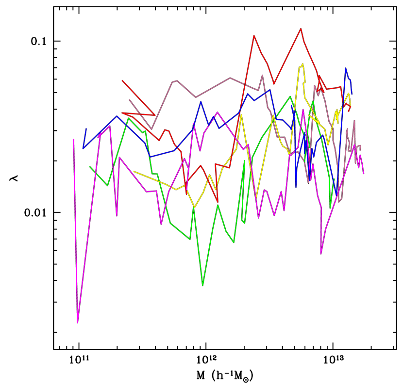
Figure 1.— Several examples of spin evolution of simulated halos. Each color represents the spin trajectory of a single main-merging tree. For the $x$ axis, we use halo mass rather than time or redshift. Halos at $z=0$ are chosen with mass $10^{13}~{}h^{-1}{\rm M_{\odot}}\leq M<2\times 0^{13}~{}h^{-1}{\rm M_{\odot}}$.

3.4. Local Environment

We define a local density measured from 10 nearest neighbor halos as a halo environment. The halos tracing the local density, called “background halos”, are all halos with mass greater than $M_{s}=10^{12}~{}h^{-1}{\rm M_{\odot}}$ (equal to the sum of 300 particle masses) at $z<7$. However, at higher redshifts ($z>7$), the number of massive halos is much lower and, therefore, we reduce the mass limit to $M_{s}=2\times 10^{11}h^{-1}{\rm M_{\odot}}$ at $7\leq z<9$ and even further to $M_{s}=10^{11}h^{-1}{\rm M_{\odot}}$ at $z\geq 9$.

The variable-width spline kernel is adopted to adaptively resolve high-density regions as

$$\rho^{i}=\sum_{j=1}^{N_{\rm n}=10}W(|{{\boldsymbol{r}}^{ij}}|/h^{i}),$$ (11)

where ${\boldsymbol{r}}^{ij}$ is the distance from the $i$th halo to the $j$th background halo, and $h^{i}$ is the distance to the tenth nearest neighbor. The density measure was first used with 20 neighbors in Park et al. (2007). The kernel size varying with environments helps dense regions not to be oversmoothed.

The spline kernel has the form

$$W(x)={8\over\pi}\begin{cases}1-6x^{2}+6x^{3}&\text{if }0\leq x\leq{1\over 2},\\ 2(1-x)^{3}&\text{if }{1\over 2}<x\leq 1,\text{ and}\\ 0&\text{if }x>1,\end{cases}$$

where $x\equiv r/h$. The median radius of the kernel is $h=7.5$ h${}^{-}1$Mpc.

The local environment is parameterized by

$$\Delta\rho_{10}(r)\equiv{\rho_{10}(r)\over\bar{\rho}}$$ (12)

where $\bar{\rho}$ is the mean density of the background halos, which is measured to be $3.54\times 10^{-3}(\rm h^{-1}\rm Mpc)^{-3}=(6.56\rm h^{-1}\rm Mpc)^{-3}$. If a region has a density of $\Delta\rho_{10}<0.7$, then we refer to it as an under-dense or void region. Regions $0.7\leq\Delta\rho_{10}<2$, $2\leq\Delta\rho_{10}<10$, $10\leq\Delta\rho_{10}<100$, and $\Delta\rho_{10}>100$ are referred to as mean-field, group, cluster, and highly clustered regions, respectively.

4. Probability Distribution of Angular Momentum Change, $P(D)$

4.1. General Descriptions of $P(D)$

Table 3Parameter ranges applied to the measurement of $P(D)$

id	halo mass ($M_{12}$)	$\lambda$	$\Delta\log_{10}M$	$\Delta\rho_{10}$	$z$
1	0.1	0.004	-0.3	0.7	5
2	0.3	0.006	-0.1	2	4
3	0.5	0.0085	-0.07	10	3
4	0.8	0.01	-0.05	100	2
5	1	0.015	-0.03	$\infty$	1.5
6	2	0.02	-0.02	-	1
7	4	0.025	-0.01	-	0.6
8	5	0.03	-0.0065	-	0.4
9	7	0.035	-0.004	-	0.2
10	10	0.038	0	-	0.0
11	20	0.04	0.004	-	-
12	50	0.043	0.0065	-	-
13	500	0.045	0.008	-	-
14	5000	0.047	0.01	-	-
15	$\infty$	0.05	0.015	-	-
16	-	0.053	0.02	-	-
17	-	0.056	0.03	-	-
18	-	0.06	0.05	-	-
19	-	0.063	0.08	-	-
20	-	0.067	0.1	-	-
21	-	0.07	0.15	-	-
22	-	0.072	0.2	-	-
23	-	0.075	0.3	-	-
24	-	0.078	0.7	-	-
25	-	0.08	$\infty$	-	-
26	-	0.09	-	-	-
27	-	0.1	-	-	-
28	-	0.11	-	-	-
29	-	0.12	-	-	-
30	-	0.13	-	-	-
31	-	0.15	-	-	-
32	-	0.17	-	-	-
33	-	0.2	-	-	-
34	-	0.25	-	-	-
35	-	0.3	-	-	-
36	-	0.4	-	-	-
37	-	0.5	-	-	-
38	-	0.7	-	-	-
39	-	1.2	-	-	-
40	-	$\infty$	-	-	-

We measured the distribution of angular momentum changes, $P(D)$, as a function of $M$, $\lambda$, $\Delta\log_{10}M$, $z$, and $\Delta\rho_{10}$. First, we divided all of the merging events into five-dimensional subsamples stretching over the entire parameter space, and measured the distribution of $D$ in each subsample. The $D$ was derived by estimating the changes in mass and the angular momentum (Eq. 10). Between merging steps ($t_{1}$ and $t_{2}$), the log mass change would be $\log_{10}M_{2}-\log_{10}M_{1}$ and the angular momentum change in the log scale is obtained as $\log_{10}|\boldsymbol{J}_{2}|-\log_{10}|\boldsymbol{J}_{1}|$, where subscripts 1 and 2 indicate the time step. Then, we fit the distribution with a bimodal Gaussian function as

$$P ( D;\mu_{1},\sigma_{1},\mu_{2},\sigma_{2})={f_{1}\over\sqrt{2\pi\sigma_{1}^{2}}}\exp\left[{-{1\over 2}{{(D-\mu_{1})}^{2}\over\sigma_{1}^{2}}}\right]$$ (13)

$$+{1-f_{1}\over\sqrt{2\pi\sigma_{2}^{2}}}\exp\left[{-{1\over 2}{{(D-\mu_{2})}^{2}\over\sigma_{2}^{2}}}\right]$$

where $\mu$ is the Gaussian mean, and $\sigma$ is the standard deviation. The overall mean ($\mu_{D}$) and standard deviation ($\sigma_{D}$) are obtained as

$$\mu_{D} = f_{1}\mu_{1}+(1-f_{1})\mu_{2}$$ (14)

$$\sigma_{D} = f_{1}\left(\sigma_{1}^{2}+d_{1}^{2}\right)+(1-f_{1})\left(\sigma_{2}^{2}+d_{2}^{2}\right),$$ (15)

where $d_{1}\equiv\mu_{1}-\mu_{D}$ and $d_{2}\equiv\mu_{2}-\mu_{D}$.

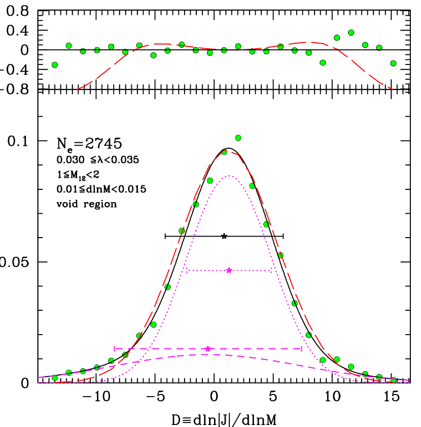
Figure 2.— Typical example of a distribution of $D$. In this plot, we select a sample with $10^{12}\leq M/(h^{-1}{\rm M_{\odot}})<2\times 10^{12}$, $0.03\leq\lambda<0.035$, $0.01\leq\Delta\log_{10}M<0.015$, and $\Delta\rho_{10}<0.7$ in the redshift interval of $0\leq z<0.2$. A total of 2745 mass events are recorded in these parameter spaces. Bottom: The solid line with symbol and error bar shows the least $\chi^{2}$ fit, mean, and standard deviation of the distribution. Also, we plot the mean and standard deviation of each Gaussian component using dotted (major component) and dashed (minor component) lines. Their corresponding Gaussian components are shown using the same line styles. The long dashed line is a single Gaussian fit to the symbols. Top: the deviations of $P(D)$ with respect to the bimodal Gaussian fit are shown with circles.

Figure 2 shows an example of the probability distribution of angular momentum change in a void sample ($\Delta\rho_{10}<0.7$) with parameter ranges $0.03\leq\lambda<0.035$, $0.01\leq\Delta\log_{10}M<0.015$, and $1\leq M_{12}<2$, where $M_{12}\equiv M/(10^{12}~{}h^{-1}{\rm M_{\odot}})$. A fitting to the bimodal Gaussian is shown by a solid line. The star symbol with a solid error bar in the middle of the plot represents the mean with 1–$\sigma$ standard deviation, while the lower two error bars (dotted and dashed) mark those of each Gaussian component. Also, we overplot the single Gaussian fit (long dashed curve), which shows a poorer fit to the fat tails on both sides (more easily seen in the upper panel). Spin distributions generated based on the single Gaussian fitting function show large deviations from simulated distributions, while the bimodal Gaussian has a better result in describing simulated spin distribution at most redshifts.

There are several points to note in this plot. First, the distribution around a peak is well described by a single major Gaussian, while the fat tails on both sides require an additional minor broad Gaussian. Second, the peak positions of the Gaussian components are not well separated from each other, implying that the combined distribution is somewhat symmetric. Most subsamples show this kind of distribution, although several show significant deviations from a symmetrical shape. Such asymmetric distributions of $D$ may play a crucial role in distorted cluster spin distributions from a log-normal form, which will be discussed in subsequent sections.

4.2. Comparison of $P(D)$ among Halo Subsamples

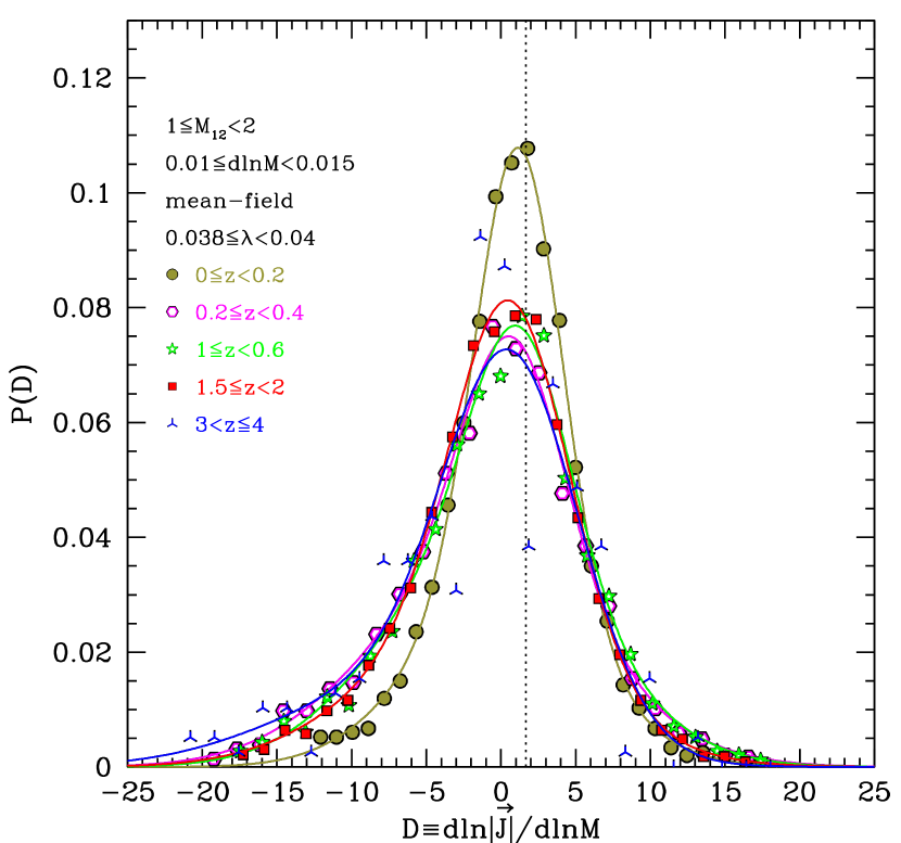
Figure 3.— Redshift evolution of $P(D)$ for a spin range of $0.038\leq\lambda<0.04$ (in a moderately rotating case). Other parameter ranges of the sample are shown in the legend. The vertical dotted line marks $D=D_{c}$ as a reference.

In Figure 3, we show the redshift dependence of $P(D)$ in halo subsamples for a small mass infall ratio ($0.01\leq\Delta\log_{10}M<0.015$) and an average spin value ($0.038\leq\lambda<0.04$) in the mean field ($0.7\leq\Delta\rho_{10}<2$). As the redshift approaches zero, the standard deviation of the distribution becomes narrower and the mean value becomes larger. From this behavior, we understand that the infall direction is more likely to be random at higher redshift because $\mu_{D}\simeq 0$ (see the distribution color-coded in blue at redshift between $z=$ 3 and 4). At a lower redshift, angular momentum changes tend to be larger, suggesting that the orbital angular momentum of infalling matter tends to be a bit more aligned with (or positively biased to) the halo rotational axis (also see Appendix B). If $D\simeq D_{c}$ (vertical dotted line), then we expect that there would be no substantial change in the spin value.

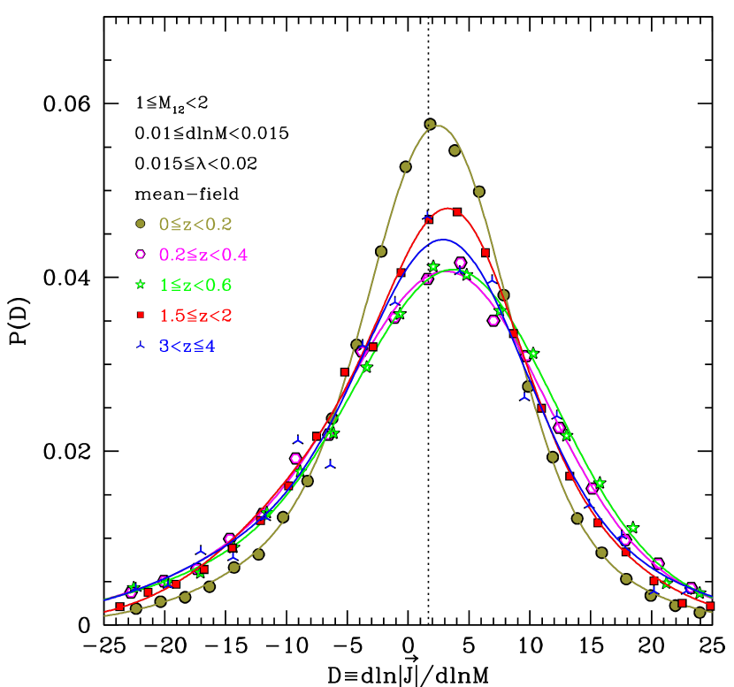
Figure 4.— Same as Fig. 3 but for low-spin sample of $0.015\leq\lambda<0.02$, which is used to isolate the spin effect on the angular momentum change.

Figure 4 shows a similar plot, but this time with slowly rotating halo samples in the accretion mode. All distributions have $\mu_{D}>D_{\rm c}$ indicating that low-spin (or slow-rotating) halos are highly likely to increase in spin value. The distribution spread is larger than in the mild-rotating samples (see Fig. 3), implying that the spin change is larger for slow-rotating halos. This is because incoming orbital angular momentum may overwhelm the previous small rotational angular momentum.

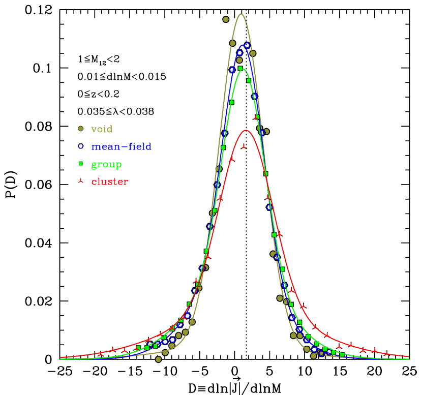
Figure 5.— Environmental dependence of $P(D)$ for the moderately rotating halo samples used in Fig. 3.

Next, we investigate the effect of environment on $D$. Figure 5 shows that halos in cluster environments experience stronger angular momentum changes inferred from larger tails (or higher probability of large-$D$ changes). This means that the angular momentum changes are statistically greater than those in lower-density regions, or that biased (or systematic) accretion or high-velocity mass infall is more frequent in cluster regions. Also, one should note that each Gaussian component has a similar peak position in most of the fittings. However, when we select a sample of higher local density, the centers of two Gaussian components begin to separate from each other. This effect on spin distribution will be described in detail in section 4.3 and 5.3.

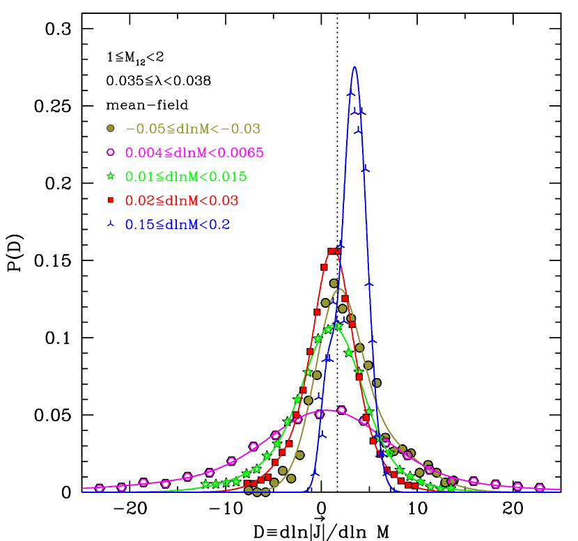
Figure 6.— Dependence of $P(D)$ on the amount of mass infall ratio ($\Delta\log_{10}M$) using samples of $1\leq M_{12}<2$, $0.7\leq\Delta\rho_{10}<2$, and $0.035\leq\lambda<0.038$.

Figure 6 provides an overall view of the effect of mass growth ($\Delta\log_{10}M$) on angular momentum change in samples of average spin values ($0.035\leq\lambda<0.038$). The average value of $D$ (or $\mu_{D}$) does not deviate much from $D_{c}$ (vertical dotted line) except in major-merging cases ($0.15\leq\Delta\log_{10}M<0.2$). The major merger significantly increases halo spin, while accretion (or minor-merger) is unlikely to produce a significant systematic change in spin for a halo. The standard deviation in the accretion mode seems to be anti-correlated with $\Delta\log_{10}M$, but the significance of the anticorrelation is a bit relaxed when weighted with the mass change (like $D\times\Delta\log_{10}M$) to update the halo spin (see Eq. 9).

4.3. Asymptotic Walk of Halo Spin

More interesting features can be obtained if one investigates the dependence of $\mu_{D}$ on sample spin. Figure 7 is a typical example showing how $\mu_{D}$ changes with sample mass and spin. By changing the sample spin while fixing other parameters, we determine the asymptotic state of the spin distribution. If $\mu_{D}>D_{\rm c}$, then the halo spin will increase; however, if $\mu_{D}<D_{\rm c}$, then the spin tends to decrease. If $\mu_{D}$ has a negative slope and crosses $D_{\rm c}$, then the spin random walk (Eq. 9) may converge to a characteristic spin value where $\mu_{D}$ crosses $D_{\rm c}$. If we define $\lambda_{\rm c}$ as a characteristic spin as $\mu_{D}(\lambda_{\rm c})=D_{\rm c}$, an the asymptotic state of the spin distribution is produced with a width depending on the shape of $P(D)$ at $\lambda=\lambda_{\rm c}$. Virtually every mass sample shows a negative slope, and the range of the characteristic spin is $0.01\lesssim\lambda_{\rm c}\lesssim 0.05$. A more massive sample tends to have a lower value of $\lambda_{c}$.

If $\mu_{D}<0$, then the rotational axis ($\boldsymbol{J}$) of the halo and the direction of the orbital angular momentum ($\boldsymbol{L}$) of infalling matter tend to be anti-correlated. However, if $0<\mu_{D}<D_{\rm c}$, then those two vectors show a positive correlation, while the mass increase is more dominant than the angular momentum increase; as a result, the halo spin decreases (see Eq. 2). If $\mu_{D}>D_{\rm c}$, then these two vectors show a strong correlation, and halo spin tends to increase accordingly. Therefore, a positive correlation between two angular momentums does not always increase the halo spin depending on the amount of angular momentum change.

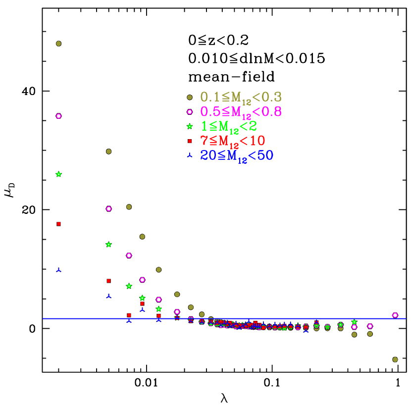
Figure 7.— Changes of $\mu_{D}$ as a function of sample mass in case of accretion ($0.01\leq\Delta\log_{10}M<0.015$). The horizontal line is $\mu_{D}=D_{c}$.

The behavior of $\mu_{D}(\lambda)$ may shape a so-called asymptotic state of the spin distribution. If a halo spin is significantly larger or smaller than $\lambda_{\rm c}$, then the halo may experience a kind of pressure toward $\lambda_{\rm c}$; as a result, the halo spin tends to move toward $\lambda_{\rm c}$. Therefore, the value of $\lambda_{\rm c}$ plays an important role in guiding the spin evolution. Of course, all halos do not immediately jump to $\lambda_{\rm c}$ but show a spread over a certain range of $\lambda$ around $\lambda_{\rm c}$, which is regulated by the shape of $P(D|\lambda=\lambda_{\rm c})$. More massive halos tend to have lower $\lambda_{\rm c}$, which means that lower spin values are preferred in more massive halo samples. This is consistent with recent findings for mass-dependent spin distributions (Antonuccio-Delogu et al., 2010; Knebe & Power, 2008; Bett et al., 2007).

Figure 8 demonstrates how the characteristic spin ($\lambda_{c}$) has varied with the infall mass ratio ($\Delta\log_{10}M$) in recent epochs ($0\leq z<0.2$). Broadly speaking, the halo spin tends to increase as the local density increases and accretions are less likely to increase the spin value as much as major mergings at the same local density; meanwhile, a less massive halo tends to have a larger spin value at the same mass increase ($\Delta\log_{10}M$). In void regions, halos have the lowest value of $\lambda_{\rm c}$. From this description, we conclude that $\mu_{D}$ in lower density regions tends to be lower than that in higher density regions (or less-aligned infall directions), and accretion may favor a less biased infall direction lowering the characteristic spin. Also, smaller cluster halos tend to have more aligned mass infalls (or a higher value of $\lambda_{\rm c}$) than larger cluster halos. The environmental dependence of $\lambda_{\rm c}$ is more clearly observed in the case of higher $\Delta\log_{10}M$.

The redshift dependence of $\lambda_{\rm c}$ can be observed by comparing Figure 8 ($0\leq z<0.2$) with Figure 9 ($2\leq z<3$). The dependence of $\lambda_{\rm c}$ on the halo mass at a given local density is relatively negligible, especially for major merging at high redshifts. Overall, $\lambda_{\rm c}$ values at $2\leq z<3$ are lower than those for $0\leq z<0.2$ cases, especially for $\Delta\log_{10}M>0$. The environmental dependence becomes stronger at lower redshifts.

We consider the frequencies of two infall scenarios (accretion or major merging) in Figure 10. Accretion ($0\leq\Delta\log_{10}M<0.1$) at low redshift ($0\leq z<0.2$, left panels) is more frequent than at the higher redshift ($2\leq z<3$, right panels). Moreover, halos in less dense regions at low redshifts are likely to have less frequent major-merging events; this environmental dependence is not observed at high redshifts. Therefore, we conclude that major-merging events subside with time, and this tendency becomes stronger in lower density regions. This may be due to the accelerating expansion of the universe at lower redshifts. The acceleration may reduce the number of major-merging events; therefore, accretion would be a dominant source of mass increase in recent epochs. Lower-density regions, especially voids, may suffer more seriously from such acceleration.

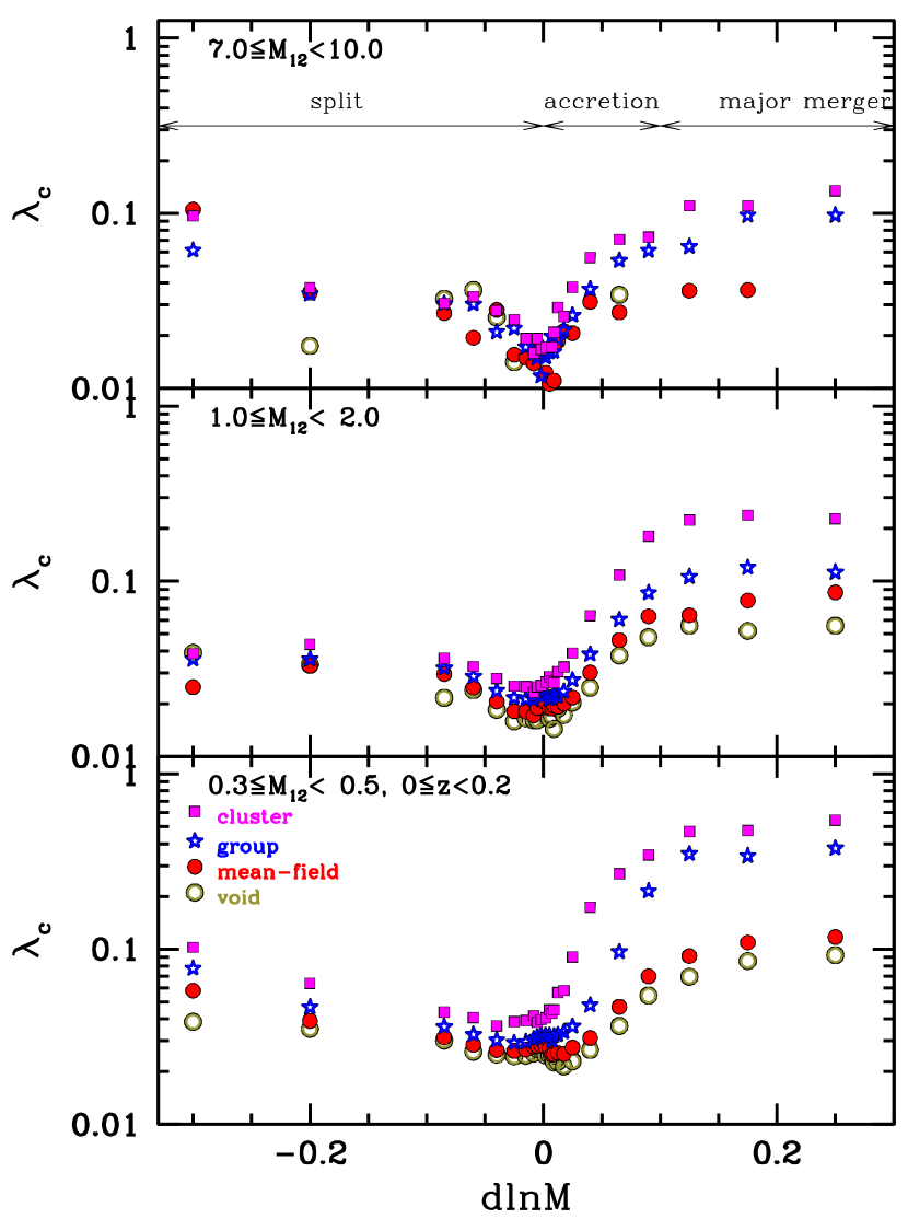
Figure 8.— Dependence of $\lambda_{c}$ on merging mass ($\Delta\log_{10}M$) between $0\leq z<0.2$ for three mass samples: $0.3\leq M_{12}<0.5$ (bottom panel), $1\leq M_{12}<2$ (middle), and $7\leq M_{12}<10$ (top). Symbols with different colors are used to distinguish the effect of local environment.

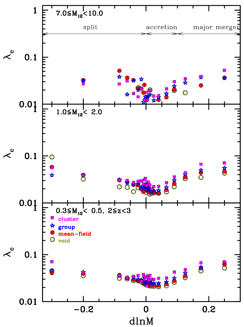
Figure 9.— Same as Fig. 8 but for redshift samples of $2\leq z<3$.

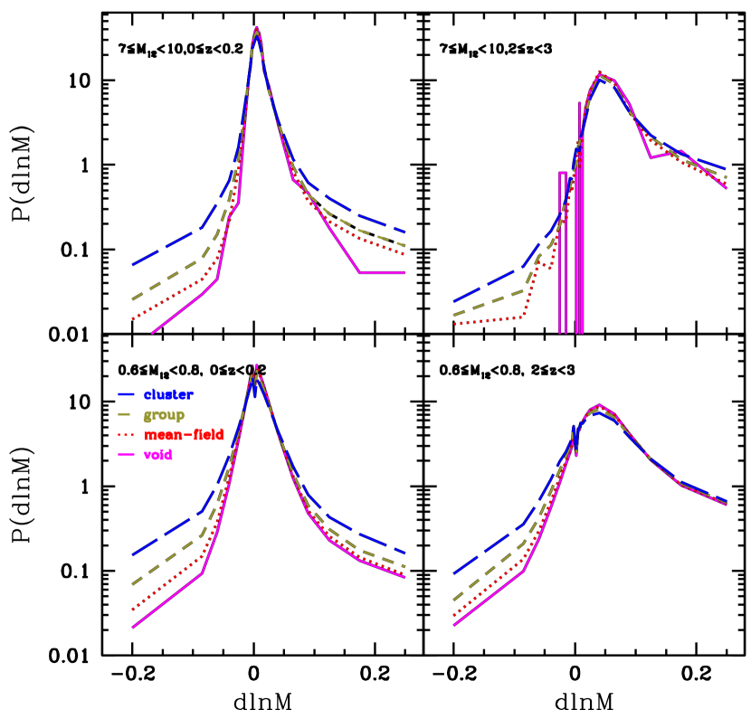
Figure 10.— Distribution of $d\log_{10}M$ for halo samples of $0.6\leq M_{12}<0.8$ (bottom panels) and $6\leq M_{12}<10$ (top) at $0\leq z<0.2$ (left panels) and $2\leq z<3$ (right).

4.4. Random Walk and Correlated Mass Infall

We need to clarify two confusing terms: random walk and correlated (or biased) infall. In this study, a random walk means that the angular momentum change at a given merging step is purely stochastic, obeying the distribution of $D$. However, the $D$ distribution (or $P(D)$) has, in most cases, has a finite mean value: a positive bias ($\mu_{D}>0$) or negative bias ($\mu_{D}<0$). The correlated infall direction indicates a preferential direction for mass infall with respect to the halo rotation axis (or its spin axis; see Appendix B for details) and does not conflict with the random-walk hypothesis.

Since $\mu_{D}$ is finite (and mostly positive), the orientations of the orbital angular momentum of infalling matter are not perfectly random but are somewhat correlated or anti-correlated with the halo rotational axis (or the direction of the angular momentum vector). However, it should be noted that as the halo spin approaches zero, even a small amount of mass infall (or accretion) may significantly increase the halo spin value ($|{\boldsymbol{L}}|\gg|{\boldsymbol{J}}|\simeq 0$), which may explain the sharp increase in $\mu_{D}$ as the sample spin approaches zero (Fig. 7).

An illustration of a spin random walk is a staggering walk taken by a drunken man. Consider a half-pipe with a U-shaped cross section and, then, a group of drunken men take a walk lurching forward along the bottom of the half-pipe without mutual collisions. Here, the shape of the cross section is not fixed, and the pipe is not like $P(D)$, which varies with sample parameters. Therefore, the distribution of walker positions gradually changes to adjust itself to the cross-sectional shape of the half-pipe, and the majority of walkers are distributed near the bottom of the pipe ($\lambda_{c}$ in the halo spin walk). In the next section, we investigate the results of spin random walks and the effects of various parameters on the shape of spin distributions.

5. Random Evolution of Halo Spin

In this section, we will show how well the stochastic model reproduces distributions of halo spin measured from $N$-body simulations. The change in angular momentum is expected to be a random process with a distribution that has a bimodal Gaussian form. We assume that the spin change in each time step is independent of the previous history (a Markov process; see Bond et al. 1991 for an example applied to halo mass function) and is completely determined by the current physical status. However, it is possible that subsequent infall events can be correlated with previous events. For example, consider successive mass infalls through a local filamentary structure. In this case, the random-walk hypothesis is not satisfied. We will discuss possible correlated infalls in the latter part of this section.

5.1. Stochastic Model of Spin Evolution

First, we choose a mass history from simulated main merger trees. The initial spin value is set to $\lambda_{0}=0.01$. At each merging step, we identify $P(D)$ of a subsample with parameter ranges enclosing the current halo mass, spin, mass change, local density, and redshift. Then, from the identified $P(D)$ we randomly generate a value of $D_{\rm rand}$. From equation (9) with $D_{\rm rand}$, we calculate the change in spin ($\Delta\lambda$) and update the spin value. In the next merging step, we iterate the same process but with the updated spin value. The resulting spin value ($\lambda_{f}$) at the final redshift is obtained as

$$\lambda_{f}=\lambda_{0}+\sum_{i=1}^{N}\Delta\lambda_{i}.$$ (16)

5.2. Effect of Halo Mass on Spin Distribution

Now, we obtain the spin distribution produced by the stochastic random walk and compare it with that of $N$-body simulations.

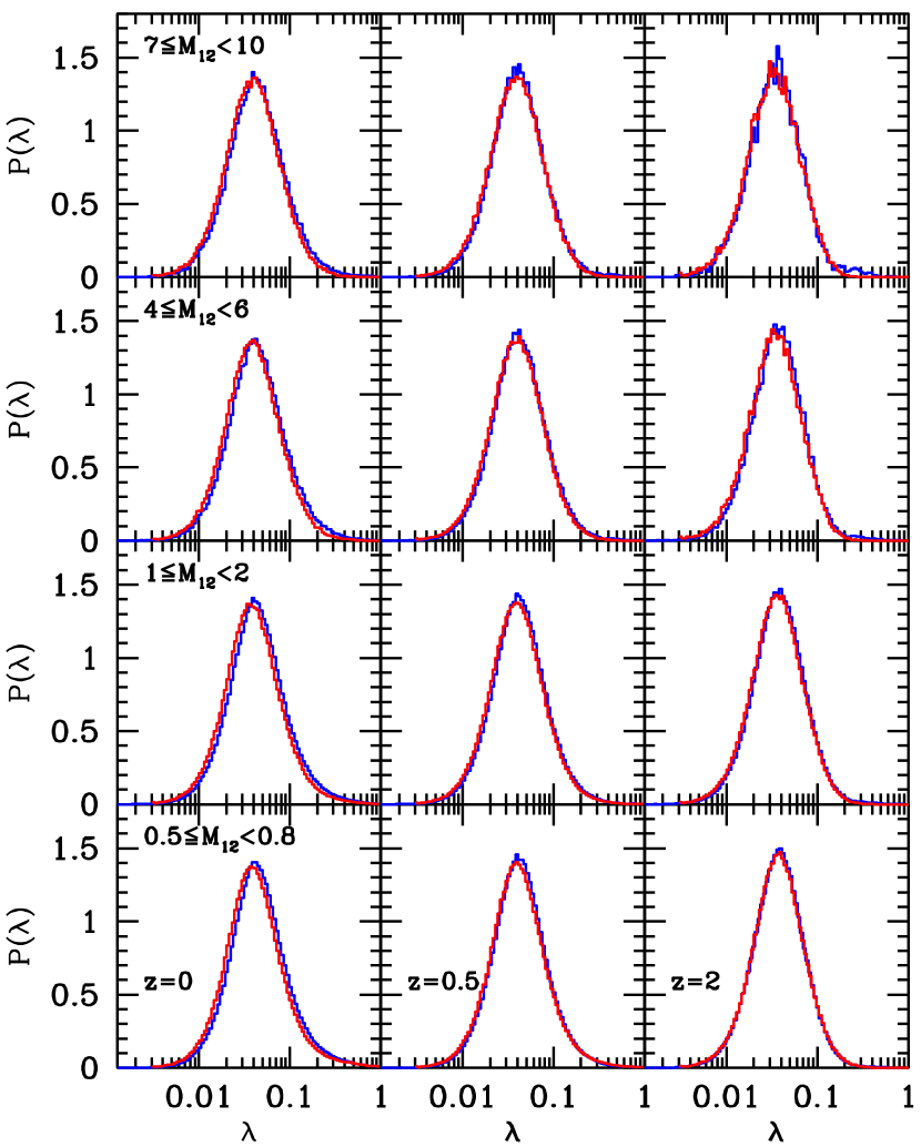
Figure 11.— Spin distributions of various halo mass samples at $z=0$, 0.5, and 2 (from left panels). The blue and red histograms are the randomly generated and $N$-body-simulated spin distributions, respectively.

Figure 11 shows the results with randomly generated spin distributions (blue histogram) against $N$-body simulated distributions (red histogram) in four mass samples. The randomly generated spin distributions at $z=0$ are similar to the simulated distributions with a slight shift to higher $\lambda$, and this difference is observed in every mass sample, although the difference is negligible at higher redshift.

In Table 4 in Appendix F, the log-normal fitting results for randomly generated and simulated spin distributions are given with a mean value, standard deviation, and $\chi^{2}$/degrees of freedom (dof). This difference is more clearly shown in Figure 12, where the blue and red histograms are the distributions of the random and simulated spins at $z=0$, respectively. The green curve is a Gaussian fit to the simulated spin distribution. Before jumping to a detailed comparison, it would be valuable to note that $N$-body-simulated halos overpopulate at the high-$\lambda$ tail (the same feature is also observed for the generated spin distributions) compared to the log-normal fitting (solid curve), which has also been found in other studies (Bett et al., 2007; Shaw et al., 2006), unless a correction is applied to the halo samples (Davis et al., 2011; Shaw et al., 2006). In Figure 13, we show the difference ($\delta_{P(\lambda)}\equiv(P_{r}-P_{s})/P_{s}$) between the simulated ($P_{\rm s}$) and randomly generated ($P_{\rm r}$) spin distributions. The differences increase as redshift decreases, while deviations in the randomly generated spin distributions at $z=0.5$ and 2 are confined within about 10–15% error.

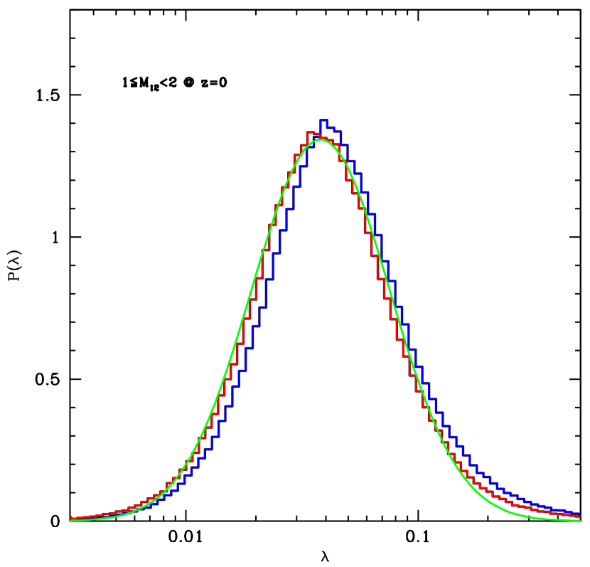
Figure 12.— Spin distributions of the mass sample of $1\leq M_{12}<2$ at $z=0$. Blue and red coded histograms are the randomly generated and $N$-body spin distributions, respectively, and the green curve shows the log-normal fit to the $N$-body histogram.

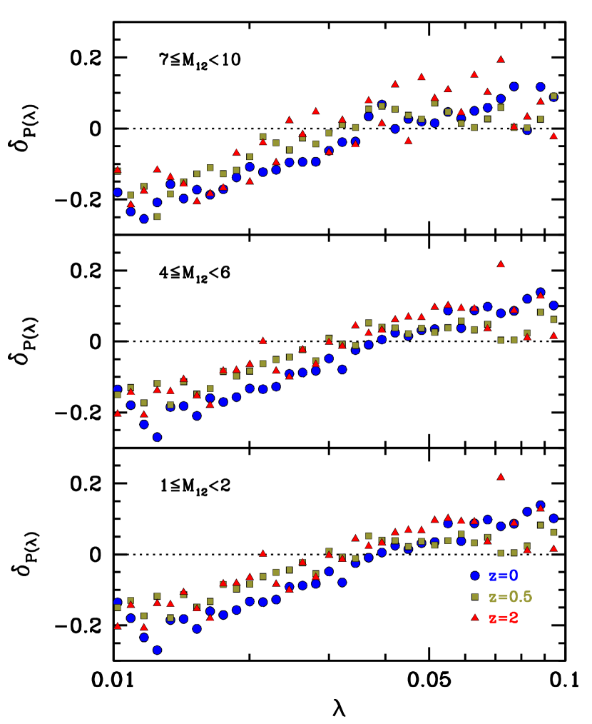
Figure 13.— Deviations in spin distribution for three mass samples measured in the spin interval of $0.01\leq\lambda<0.1$. The circles, boxes, and triangles are measured at $z=0$, 0.5, and 2, respectively. We removed the irrelevant regions of $\lambda<0.01$ and $\lambda>0.1$ as the number of simulated halos in those regions is very small.

5.3. Environmental Effect on Spin Distribution

If a spin walk is well described by the Markov (or random) process and a sufficient number of trials are performed to suppress the Poisson error, then the $N$-body-simulated and randomly generated spin distributions should be basically equal to each other. Therefore, a subtle failure in recovering the simulated spin distribution at lower redshifts, as seen in Figure 11, may imply a possible limitation of the stochastic model.

A possible explanation for the mismatch of spin distributions between the simulation and the stochastic model is correlated mass merging, which means a subsequent mass infall changes the angular momentum of a halo in the same direction. Then, a set of $D_{\rm rand}$s in the successive infalls may not be random but correlated. This correlated mass merging could be a function of local environment. In void regions, halos are likely to have fewer major mergers, while those in cluster regions may experience more frequent heavy mass infalls (see Fig. 10). Because it is believed that major mergers frequently occur when clumps of matter fall along filamentary structures, the number of filaments connected to a halo determines whether or not the spin walk is random. In void regions, filamentary structures are relatively rare and void halos tend to have a small number of filaments around them, which means that subsequent major mergers may occur along a smaller number of filamentary structures.

Figures 14–16 show the environmental effect on spin distribution at three redshifts. In Table 5 of Appendix F, the log-normal fitting results are listed. We clearly see that a randomly generated spin (blue histogram) tends to substantially overestimate the halo spin of the $N$-body-simulation in lower density regions.

For the group and cluster samples, the difference in spin distributions between the simulation and the stochastic model is relatively small. However, with time the difference increases with time and the group sample begins to show such a discrepancy at $z=0$.

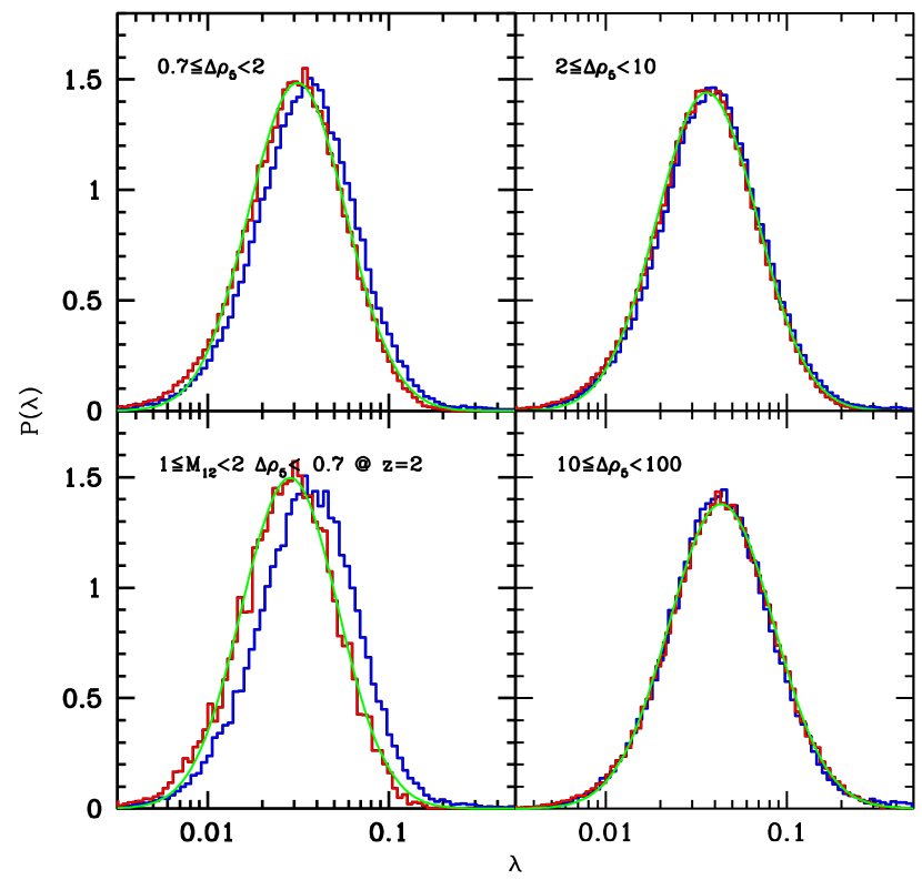
Figure 14.— Spin distributions in various local environments at $z=2$. Counterclockwise from the bottom left panel are the spin distributions of $N$-body (red histogram) and random-generated (blue) samples of local densities of $\Delta\rho_{10}<0.7$, $0.7\leq\Delta\rho_{10}<2$, $2\leq\Delta\rho_{10}<10$, and $10\leq\Delta\rho_{10}<100$. The green solid curve in each panel is a log-normal fit to the $N$-body spin distribution.

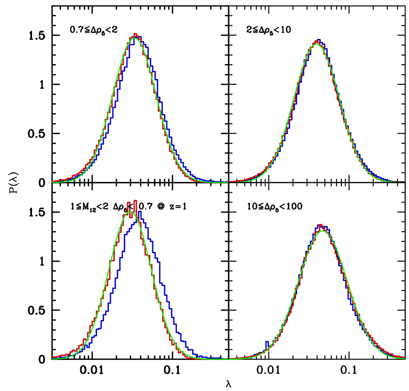
Figure 15.— Same as Fig. 14 but at $z=1$.

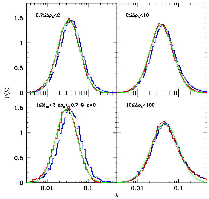
Figure 16.— Same as Fig. 14 but at $z=0$.

Since a massive halo is likely to be located in a knot (interconnection) of local filamentary structures, the probability of successive major mergers along a single filament is low (the next major merger may occur with another filamentary structure). Therefore, it would be interesting to determine whether the randomly generated halo spins of more massive samples have a distribution similar to that of the $N$-body simulation. In Figure 17, we show the generated spin distributions of a massive sample of $6\leq M_{12}<10$ in different local environments. No substantial difference is shown even in void regions. Therefore, it is quite reasonable to believe that massive halos tend to show random evolution in spin.

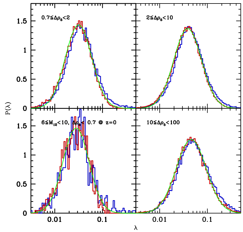
Figure 17.— Spin distributions of a more massive sample of $6\leq M_{12}<10$ at $z=0$. The green solid curve is a log-normal fit to the corresponding $N$-body distribution.

In these figures, the halo spin distribution depends on the local environment; denser regions cause halos to rotate faster, which is also confirmed in Figure 8 ($\lambda_{\rm c}$ is higher in a denser region). Also, most of the spin samples show log-normal distributions, except for the cluster samples at $z=0$, where the distribution has a slightly fat tail at larger $\lambda$. This may be due to unrelaxed halos in cluster regions where violent mergers are so frequent that cluster halos do not have sufficient time to transfer angular momentum to outside and finally to be virialized.

6. Markovian and Non-Markovian Processes

Throughout this paper, the stochastic model we adopted assumes that the spin walk can be described by the Markov process, which requires that a random walk be memoryless or independent of previous states. Therefore, it is important to determine whether the spin walk observed in $N$-body simulations is really random (Markovian) or not (non-Markovian).

6.1. Autocorrelation between Neighboring Mass Events

One of the easiest ways to verify the correlation of two separate events in a halo merging history is to measure the autocorrelation (or serial correlation) between a pair of events in a main merger tree line. The first-order autocorrelation of two mass events of $i$ and $j$ is

$$\Xi(i,j)={{w_{i}w_{j}\left({D_{i}-\mu_{i}\over\sigma_{i}}\right)\left({D_{j}-\mu_{j}\over\sigma_{j}}\right)}}$$ (17)

where $w$ is a weight, $D$ is randomly generated by the stochastic model or provided by simulations, $\mu$ is the mean, and $\sigma$ is the standard deviation of the probability distribution of $D$. In this analysis, we adopt $w_{i}=|\Delta\log_{10}M_{i}|$ and define the lag-$k$ autocorrelation as

$$C_{k}(z)={1\over{\mathcal{W}}_{\rm pair}}\sum_{i,j=i+k}{\Xi(i,j|\geq z)},$$ (18)

where ${\mathcal{W}}_{\rm pair}=\sum w_{i}w_{j}$ and the summation is performed over all possible lag-$k$ pairs of events in a halo history to redshift $z$. Only a relative comparison is possible because the time interval between a lag-$k$ pair changes.

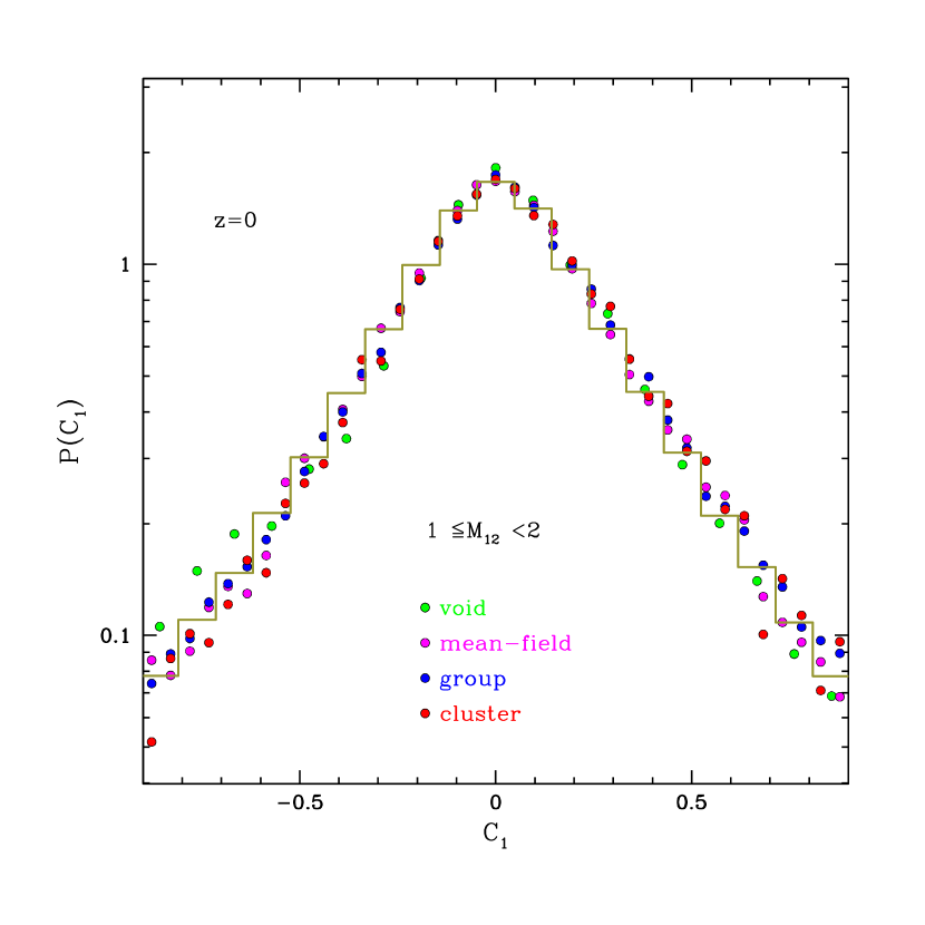
Figure 18.— Example of the probability distribution of $C_{1}$ (Eq. 18) in a sample of $1\leq M_{12}<2$ at $z=0$. The symbols are distributions measured with the spin history of the $N$-body halo sample with $\Delta\rho_{10}<0.7$ (green), $0.7\leq\Delta\rho_{10}<2$ (magenta), and $2\leq\Delta\rho_{10}<10$ (blue). The histogram shows the mean distribution of 100 random generations in the sample of $\Delta\rho_{10}<0.7$.

Using 100 random realizations of $P(C_{k})$, we statistically measured the deviation of the autocorrelations of $N$-body data from random expectations. The probability distribution of a lag-one autocorrelation is shown in Figure 18 for halo samples of $1\leq M_{12}<2$ in four local-density regions (colored symbols). The brown histogram is a mean expectation measured from the 100 random realizations. Even though the probability distribution of $D$ depends on the local density, the autocorrelation seems to be indistinguishable between different local-density samples and even from the random model in this plot.

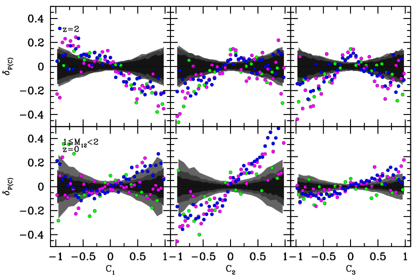
Figure 19.— Randomness check by the measurement of autocorrelations, $C_{1}$ (left panels), $C_{2}$ (middle), and $C_{3}$ (right) in the sample of $1\leq M_{12}<2$ at $z=0$ (bottom panels) and 2 (top). The three gray levels in the regions are the 1–$\sigma$ distributions of 100 random generations for $\Delta\rho_{10}<0.7$ (outer gray region), $0.7\leq\Delta\rho_{10}<2$ (middle), and $2\leq\Delta\rho_{10}<10$ (innermost) with corresponding $N$-body estimations plotted with green, magenta, and blue circles, respectively.

We also showed deviations between simulated correlations and the random model with $\delta_{P(C_{k})}\equiv(P_{s}(C_{k})-P_{<r>}(C_{k}))/P_{<r>}(C_{k})$, where $P_{s}(C_{k})$ is the simulated autocorrelation and $P_{<r>}(C_{k})$ is the average of the 100 randomly generated autocorrelations. Figure 19 shows the results for a sample of $1\leq M_{12}<2$. The shaded region depicts the 1$\sigma$ distributions of the random model, and the symbols are measured from $N$-body simulations. It is easy to see the negative autocorrelations of $C_{1}$ at $z=2$ and the positive correlations of $C_{2}$ at $z=0$ with greater than 2$\sigma$ confidence limits. We further investigated autocorrelations from $C_{4}$ to $C_{6}$ but found nothing substantially deviating from the random model. On the other hand, we could not detect any possible autocorrelations in the massive sample ($6\leq M_{12}<10)$). Most of the simulated autocorrelations are contained within 1$\sigma$ random expectations (see Fig. 20).

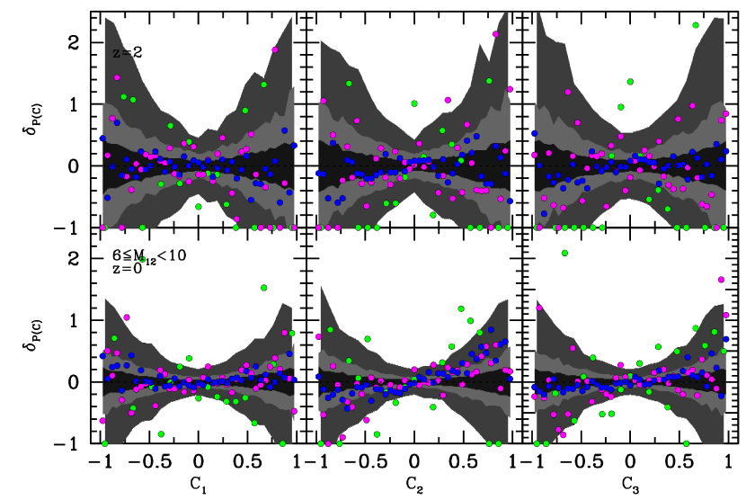
Figure 20.— Same as Fig. 19 but for the massive samples of $6\leq M_{12}<10$. Due to the smaller sample size, the 1–$\sigma$ scatter of the random sample is larger than that of the sample of $1\leq M_{12}<2$.

Detecting substantial autocorrelations of $C_{1}$ at $z=2$ and $C_{2}$ at $z=0$ may provide a tangible clue for void discrepancies between the simulated and generated spin distributions. Correlated infall events may cause void halos to have smaller spin values, but we are unable to detect any environmental dependence in the correlation figure. However, considering the frequent major merging of cluster halos, an autocorrelation could easily be counterbalanced by other major-merging events. However, the void halos have little possibility of another major merging.

6.2. Origin of the Log-normal Distribution of Halo Spin

In this subsection, we demonstrate that the log-normal distribution is a natural consequence of the stochastic differential equation in the stochastic of halo spin. In many studies, simulated spin distributions in various mass samples consistently show substantial deviations from the log-normal form in the high-$\lambda$ tail. However, no serious deviations are found as long as a mass sample is further divided into local-density subsamples. As shown in Figures 14–16, the log-normal fitting functions (green curves) seem to describe well the simulated spin distributions (red histograms) in various local environments, except for cluster regions at $z=0$.

Now, consider a one-factor model of the Markov process or the model of Geometric Brownian Motion (GBM; Ross 2010), which has a stochastic differential equation of

$${d\log_{10}\lambda(\tau)\over d\tau}=\theta+\sigma_{c}{dW_{\tau}\over d\tau},$$ (19)

where $\theta$ describes the long-term drift of the system, $\sigma_{\rm c}$ is a constant, and $W_{\tau}$ is a kind of normally distributed Wiener process or $W_{\tau}\sim{\mathcal{N}}(0,\tau)$ where ${\mathcal{N}}(0,\tau)$ denotes the normal distribution with a zero mean value and a variance of $\tau$.

From the properties of the Wiener process such as $(W_{\tau_{2}}-W_{\tau_{1}})\sim{\mathcal{N}}(0,{\tau_{2}}-{\tau_{1}})$ for $\tau_{2}\geq\tau_{1}$, we obtain the probability distribution of $dW/d\tau$ as

$${dW_{\tau}\over d\tau}={W_{\tau+d\tau}-W_{\tau}\over d\tau}\sim{{\mathcal{N}}(0,d\tau)\over d\tau}={\mathcal{N}}(0,1/d\tau),$$ (20)

where the statistical relation of $\mathcal{N}(\mu,\sigma^{2})/a=\mathcal{N}(\mu,\sigma^{2}/a^{2})$ is used. Thus, the probability distribution of $dW_{\tau}/d\tau$ is a normal distribution with a zero mean and a variance of $1/{d\tau}$. The Wiener process has the following properties:

$$dW_{\tau} \sim \mathcal{N}(0,1)\sqrt{d\tau}$$ (21)

$$dW^{2}_{\tau} \sim \sqrt{2}\mathcal{N}(0,1)d\tau\propto d\tau.$$ (22)

According to Itō’s formula (Movellan, J. R., 2011), we may linearize the change of $\log\lambda$ as

$$d\log\lambda = {d\log\lambda\over d\lambda}d\lambda+{1\over 2}{d^{2}\log\lambda\over d\lambda^{2}}d\lambda^{2}$$ (23)

$$= \sigma_{c}dW_{\tau}+\left({\theta-{\sigma_{c}^{2}\over 2}}\right)d\tau$$ (24)

where we used the relation $d\lambda=\lambda(\theta d\tau+\sigma_{c}dW_{\tau})$ (from Eq. 19) and $dW{{}_{\tau}}^{2}=d\tau$ (Eq. 22), and ignored the higher-order terms of $d\tau$. By integrating the above equation, we finally obtain

$$\log\left({\lambda(\tau)\over\lambda_{0}}\right)={\sigma_{c}W_{\tau}+\left({\theta-{\sigma_{c}^{2}\over 2}}\right)\tau}.$$ (25)

Now, one can understand that the logarithm of the stochastic process $\lambda$ follows a Wiener process with a standard deviation of $\sigma_{c}$ and a corrected long-term drift of $\theta-\sigma_{c}^{2}/2$ (Øksendal (2000) for details). If $W_{\tau}$ does not have a normal distribution, then we may not obtain a logarithm of the randomly distributing quantity. For example, if $W_{\tau}$ has a probability proportional to $-\tau$ or $-\tau^{2}$, then the resulting distribution would be exponential or Gaussian, respectively.

We now attempt to combine the right two right-hand terms in equation (19) into $\mathcal{D}$ as

$${d\log_{10}\lambda(\tau)\over d\tau}=\mathcal{D},$$ (26)

where $\mathcal{D}\sim\mathcal{N}[\theta,\sigma_{c}^{2}/{d\tau}]$. After changing variables as $\tau\rightarrow\log_{10}M$ and $\mathcal{D}\rightarrow D-D_{c}$, we can find an analogy between the GBM and the angular momentum change, $D$ (see Eq. 9). Although the overall distribution of $D$ is better fit by the bimodal Gaussian, the distribution around a peak can be well modeled by a single Gaussian peak because the two Gaussian components have nearly the same center in most samples, and we may simply approximate $P(D)$ around the peak as a normal distribution. The minor Gaussian component with a broad width is mostly needed to describe the fat tails on both sides. Consequently, the distribution of $\log_{10}\lambda$ follows the normal process, which means that the spin distribution of $\lambda$ should accordingly be log-normal. If the centers of two Gaussian components are well separated, or the minor Gaussian component is comparable to the major one, then the resulting distribution of $\log_{10}\lambda$ may show a considerable deviation from the normal distribution.

Here, we need to address the validity of the application of the GBM model to spin evolution before jumping to a conclusion, and thus we test whether the halo spin change satisfies two prerequisites of the GBM model:

• $\theta$ (or $\mu_{D}$) should depend only on $\tau$ (or $\log_{10}M$); and

• the standard deviation of $\mathcal{D}$ (or $\sigma_{D}$) should be proportional to $d\tau^{-1/2}$ (or $(\Delta\log_{10}M)^{-1/2}$).

To qualitatively assess the first condition, Figures 3, 4, 5, and 6 show that there is no significant change in $\mu_{D}$ with different redshifts, local environments, or infall mass ratios, except for major-merging events, in which case a substantially larger $\mu_{D}$ is obtained. Consequently, one can easily see the mass dependence in Figure 7.

The second condition might be related to the temporal resolution affecting the mass infall ratio. Now, we investigate the following relation:

$$\sigma_{{D}}^{-1}=(\Delta\log_{10}M)^{1/2}\sigma_{c}^{-1},$$ (27)

where $\sigma_{c}$ is constant with respect to $\Delta\log_{10}M$ as long as the second requirement is satisfied. In order to obtain a log-normal distribution of $\lambda$, $\sigma_{{D}}^{-1}$ should be linearly scaled to the change in halo mass. As shown previously, the spin distribution has a mass and environmental dependences, indicating that the distribution is not stationary but evolves with the halo mass. However, halo environments do not change substantially over cosmic time since a halo does not generally move a great distance ($\lesssim$ a few Mpc). Hence, it is sufficient to examine the relation between $\sigma_{{D}}^{-1}$ and $\Delta\log_{10}M$ in the same environment.

Figure 21 shows the change in $\sigma_{{D}}^{-1}$ over a range of infall mass ratios at $z=0$. The measured relation substantially deviates from a single power-law scaling but we can divide the range of $\Delta\log_{10}M$ into three regions: $\Delta\log_{10}M<0.03$ (quiet accretion), $0.03<\Delta\log_{10}M\leq 0.1$ (strong accretion), and $\Delta\log_{10}M>0.1$ (major merging). Each region, except for the strong accretion mode, has its own power-law relation of $\sigma_{D}^{-1}\propto(\Delta\log_{10}M)^{1/2}$. The major-merging mode and quiet accretion mode have different variances in that the major-merging mode has a higher value of $\sigma_{c}$. This implies that the major merger mode has a relatively larger stochastic walk size than the quiet accretion (see Eq. 19). The transition (or strong accretion) mode ($0.03\leq\Delta\log_{10}M<0.1$) does not seem to satisfy the assumptions of the GBM model. Now we conclude that even though there exist limitations in applying the GBM model to spin evolution, the spin walk is well described by the GBM model and, consequently, the resulting spin distribution follows the log-normal function.

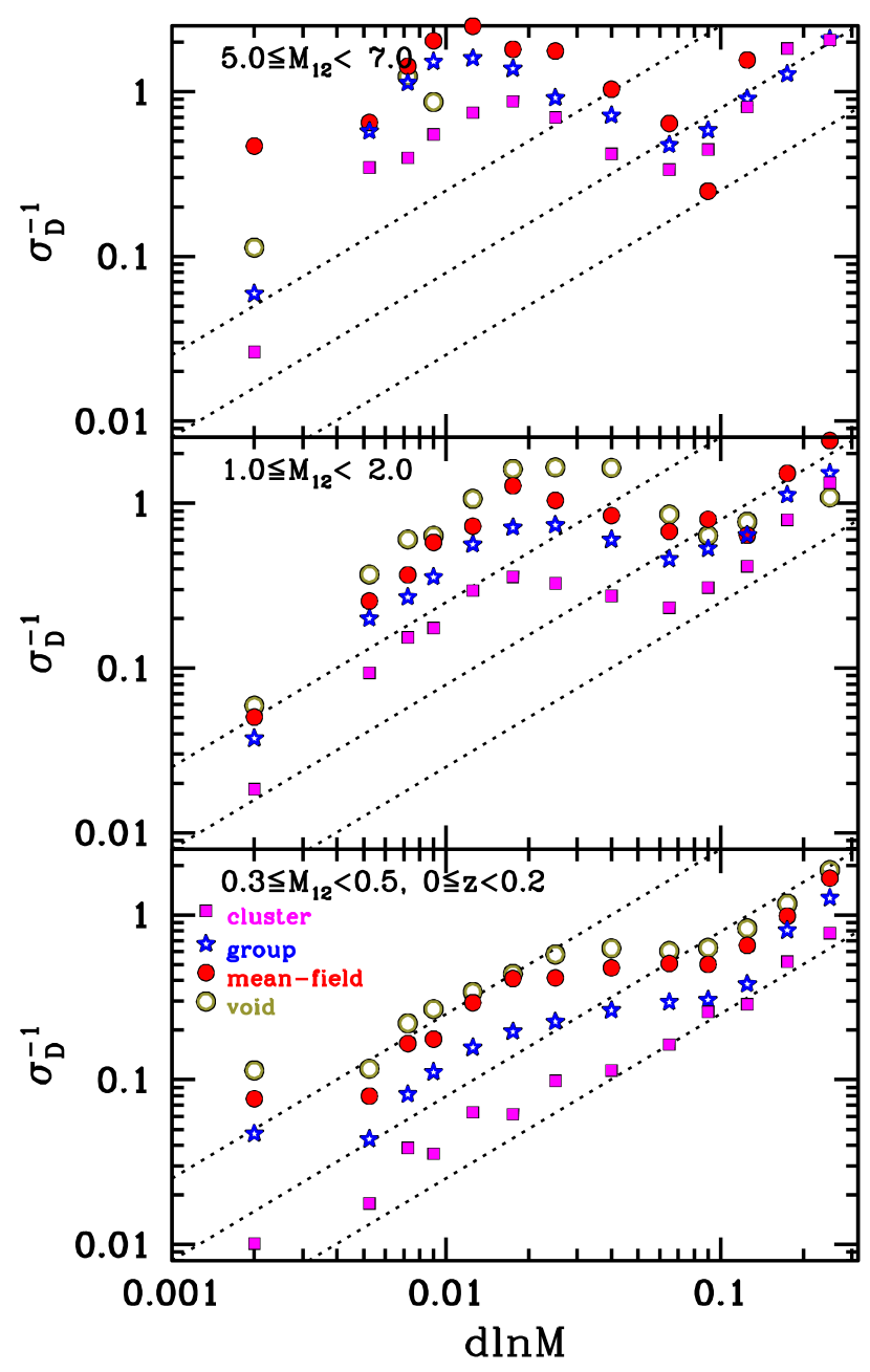
Figure 21.— Changes in $\sigma_{\mathcal{D}}^{-1}$ and infall mass ratio, $\Delta\log_{10}M$ (bottom), at $0\leq z<0.2$ for different halo masses, $0.3\leq M_{12}<0.5$ (bottom), $1\leq M_{12}<2$ (middle), and $5\leq M_{12}<7$ (top panel). The dotted lines show the linear relation between $\sigma_{{D}}^{-1}$ and $d\log_{10}M$.

7. Conclusions

We concluded that the spin distribution is well described by a random walk of angular momentum. Halos in lower density regions in recent epochs present some failures. This may be due to correlated major-merging events (see further discussions in Appendix B and C). The log-normality of the spin distribution is found to be a consequence of the stochastic random walk, and most density samples show log-normal distributions of the halo spin. Only a small departure is found in the cluster samples at $z=0$, mainly because a fraction of halos are not yet relaxed. We found that the angular momentum of a halo is likely to increase after merging, and the spin distribution depends on the sample mass. If the sample mass is higher, then the average spin value decreases. The simulated log-normal distribution of the spin is well recovered by the stochastic model with bimodal Gaussian distributions of angular momentum change.

In the standard $\Lambda$CDM model, the universe has undergone a recent accelerating expansion, making it difficult to pull nearby material into a local shallow gravitational center. Compared with the flat $\Omega_{m}=1$ model, the $\Lambda$CDM model has prominent filamentary structures lacking many small and faint structures that could be easily destroyed by the recent cosmic acceleration. This effect is even stronger in void regions where the mass evolution was already halted at higher redshifts. Therefore, the cosmological effects may leave clear evidence in the spin evolution of void halos and mean-field halos at lower redshifts ($0.7\leq\Delta\rho_{10}<$2; see the top-left panel of Fig. 16).

Because of the bimodal Gaussian shape of the angular momentum change in the stochastic model, one may raise the question of the possible existence of another hidden parameter for subsampling merging events to measure $P(D)$. By introducing another parameter, a simpler distribution shape may be obtained. A bimodal Gaussian shape could be obtained through a possible correlation among spin walks, which seems to be significant in void regions and in mean fields. This may explain the deviations in halo spin distributions from the log-normal distribution.

In this study, we directly adopt the simulated mass evolution for the halo mass change ($\Delta\log_{10}M$). There are several models for the mass merging based on the EPS formalism (Press & Schechter (1974) for the classical and Bower (1991); Bond et al. (1991); Lacey & Cole (1993); Kauffmann & White (1993); Mo & White (1996); Sheth & Lemson (1999); Sheth et al. (2001); Sheth & Tormen (2002); van den Bosch (2002); Hiotelis & Del Popolo (2006); Zhang et al. (2008); Moreno et al. (2008); Neistein & Dekel (2008); Parkinson et al. (2008); Jiang & van den Bosch (2014) for variant EPS models), which can also provide us the probability of merging phases (major merger or accretion) between time steps. Since our stochastic model may discriminate between the effects of accretion and major merging in spin distributions, we may check whether the variant EPS models may produce proper probability distributions of $\Delta M/M$ compared to simulated ones for a given time step. In Appendix G, we show the roles of major merging and accretion in shaping the spin distribution in detail by adopting a toy model with fixed the mass-merging ratio and how much the mass-merging history generated by the classical EPS model predicts different spin distributions from the $N$-body simulated ones.

Appendix A Effect of $\alpha(z)$ on Spin Distribution

$\alpha(z)$ deserves more investigation because its effect on spin distribution is not negligible. The cosmological contributions to log-spin change with a mass increase in $\Delta\log_{10}M$ are $-0.008\lesssim\alpha(z)\Delta\log_{10}M<0$ in most redshift intervals of merging data. So, even though its contribution is neglected, spin error is less than 1%. But, the error accumulates over the number of merging steps and may substantially change the spin distribution.

Figure 22 shows how the spin distribution changes when the $\alpha(z)$ term is neglected in the random walk process. The generated spin distribution is substantially shifted to higher $\lambda$, which demonstrates the sensitivity of spin walk to such a very small value or possible error in fitting $P(D)$ and how large the sample size should be to suppress this kind of a noise effect.

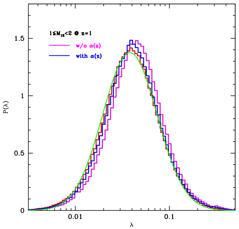
Figure 22.— Effect of $\alpha(z)$ on the spin distribution at $z=1$. The histograms colored in blue and magenta are obtained with and without $\alpha(z)$ in Eq. 8, respectively. As references, the red histogram and a green curve are the $N$-body spin distribution and its fitting function, respectively.

However, this does not guarantee that we may determine the cosmological model from the measured spin distribution because the measured $P(D)$ in this analysis may differ in different cosmological models.

Appendix B Angle Alignment between Rotational and Orbital Angular Momenta

It would be interesting to examine the angle alignment between the rotation ($\boldsymbol{J}$) of a halo and the orbital angular momentum (${\boldsymbol{L}}$) of infalling matter. If they are positively or negatively aligned, then the rotational angular momentum of a halo is expected to increase or decrease, correspondingly. Therefore, this analysis is complementary to the work on the change in angular momentum ($D$). In this section, we study two infall modes: accretion ($0\leq\Delta\log_{10}M<0.1$) and major merging ($\Delta\log_{10}M\geq 0.1$). The angle between two vectors is measured by

$$\theta_{\Delta}\equiv\cos^{-1}\left({{\boldsymbol{J}}\cdot{\boldsymbol{L}}\over|{\boldsymbol{J}}||{\boldsymbol{L}}|}\right).$$ (B1)

Figures 23, 24, and 25 show the probability distribution of $\theta_{\Delta}$ in halo samples of $0.03\leq\lambda<0.05$ (low-spi), $0.01\leq\lambda<0.03$ (average-spin), and $0.05\leq\lambda<0.3$ ( high-spin), respectively, for two mass-merging modes (the accretion in the left and major merging in the right panels). In the accretion mode, the low-spin halos (Fig. 24) are likely to have slightly negative correlations with $\theta_{\Delta}$ (anti-aligned), while average-spin halos tend to have a slightly positive alignment, and high-spin halos (Figs. 23 and 25) have a strong positive alignment. On the other hand, in major-merging mode, the low-spin, average-spin, and high-spin samples show negative, random, and positive correlations, respectively.

If two angular momentum vectors are anti-aligned, then a halo’s rotational angular momentum ($\boldsymbol{J}$) is reduced and, consequently, its spin value is lowered. Therefore, a halo with an average spin value is likely to have a slightly positive correlation to offset the negative drag term ($-5/3$), while a high-spin or low-spin halo tends to have positively or negatively aligned mass infalls, respectively. Then, the alignment of two vectors and the value of a halo spin are closely correlated with each other, producing a high spin value, and vice versa.

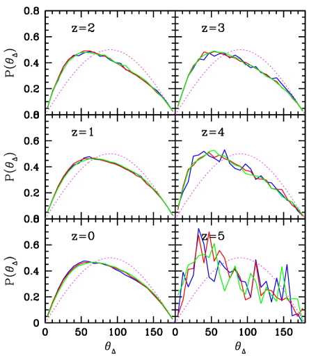
(a) accretion

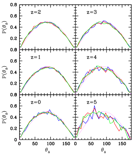
(b) merging

Figure 23.— Angle alignment between $\boldsymbol{J}$ and $\boldsymbol{L}$ of accretion (a) in major-merging events and (b) in halo samples of $0.03\leq\lambda<0.05$ and $1\leq M_{12}<2$. Counter-clockwise from the lower left panel, sample redshifts are $z=0$, 1, 2, 3, 4, and 5. Each color-coded curve is measured from the local-density sample of void (blue), mean-field (red), or group (green) regions. The magenta sine curve (dotted line) marks the random orientation.

2

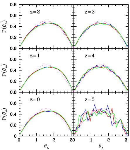
(a) accretion

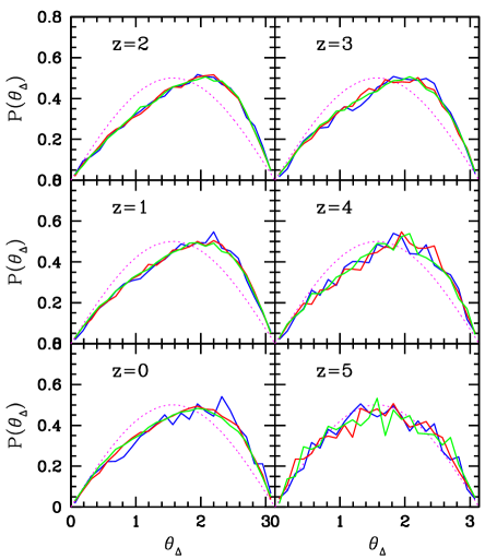
(b) merging

Figure 24.— Same as Fig. 23 but for slowly rotating samples of $0.01\leq\lambda<0.03$.

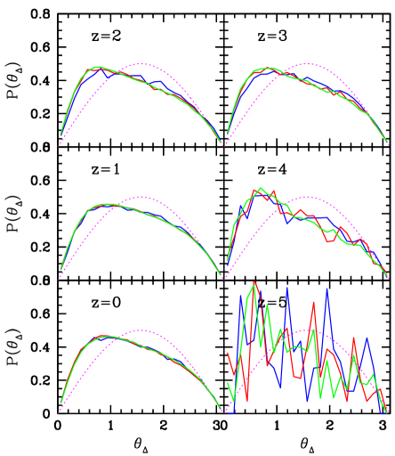
(a) accretion

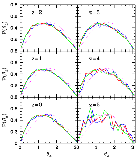
(b) merging

Figure 25.— Same as Fig. 23 but for fast-rotating samples of $0.05\leq\lambda<0.3$.

Appendix C Angle Correlations between Mass Events

This section discusses testing to determine whether or not the directions of the orbital angular momenta of infalling matter in two events are correlated. The angle between the orbital angular momenta in the $i$th and $j$th events is defined as

$$\theta_{ij}\equiv\cos^{-1}\left({{\boldsymbol{L}}_{i}\cdot{\boldsymbol{L}}_{j}\over|{\boldsymbol{L}}_{i}||{\boldsymbol{L}}_{j}|}\right),$$ (C1)

and we apply a weighting of $w_{i}=\Delta\log_{10}M$ placing more weight on major-merging pairs. We only consider $j=i+1$ cases. Figures 26– 28 show the directional correlations of the slowly, mildly, and fastly rotating halos, respectively. In the figures, there is no explicit dependency on environment. Slow-rotating halos show a negative correlation (anti-aligned) with regard to the direction of $\boldsymbol{L}$ between two successive events, which explains why they are slowly rotating. However, some interesting features can be found in the mildly and fastly rotating samples, which develop a strong anti-correlation at lower redshift ($z\leq 1$; bottom-left panel of Figs. 27 and 28). This may curb the development of spin as a whole and may explain the reason why void halos seem to have a non-Markovian walk of $D$. Halos in denser regions are expected to experience frequent major mergers. Thus, even though there is anti-alignment between two steps, the many other major merger events violently erase the memory of previous anti-correlations. Therefore, the superpositions of multiple anti-correlations are completely mixed and may result in a random-like process. However, void halos tend to experience relatively few major mergers, and the effect of anti-alignment in a rare pair of merging events may survive for a longer time. This may explain why void halos are not properly described by the stochastic random walk of $D$. We discuss the number of major mergers a halo may experience during its life time in Appendix E.

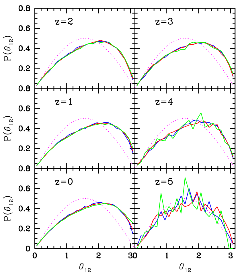
Figure 26.— Angle correlations ($\theta_{12}$) of orbital angular momenta for subsequent mergings in slow-rotating samples with $0.01\leq\lambda<0.03$. Each color-coded curve is measured from the local-density sample of void (blue), mean-field (red), or group (green) halos. The magenta sine curve (dashed line) marks the average expectation of random orientations.

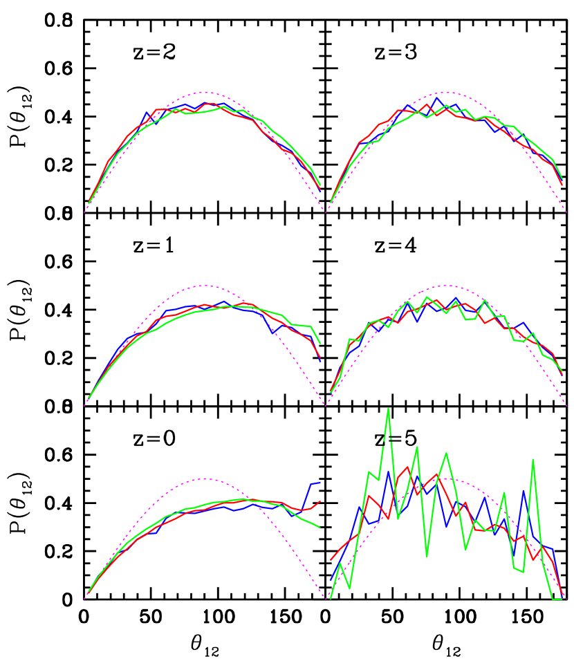
Figure 27.— Same as Fig. 26 but for the mildly rotating sample with $0.03\leq\lambda<0.05$.

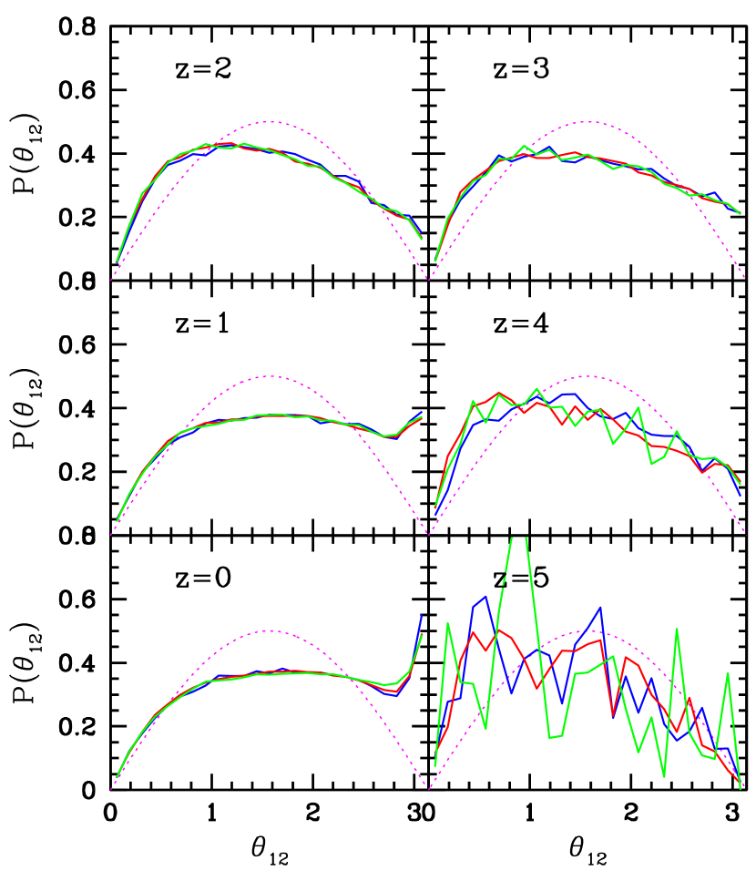
Figure 28.— Same as Fig. 26 but for the fastly rotating sample with $0.05\leq\lambda<0.3$.

Appendix D Autocorrelations between Major Mergers

We estimate the autocorrelation between a pair of nearest major merger events to determine whether substantial amounts of correlation could be detected. In this case, we only consider autocorrelations between major merger events. The deviations of autocorrelations between major mergers ($C_{\rm mm}$) are shown in Figure 29 for several redshifts. In this figure, major merger autocorrelations at high redshifts ($z\geq 2$) are equivalent to the random distributions, while weak positive correlations are detected ($\simeq 1\sigma$) at lower redshifts. More massive samples do not show any positive or negative correlations, as seen in panel (b) of Figure 29. Therefore, in this plot, we are sure that there is no substantial autocorrelation between major mergers.

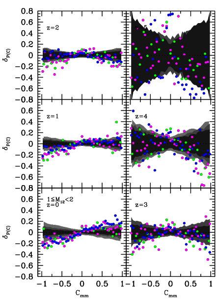
(a) $1\leq M_{12}<2$

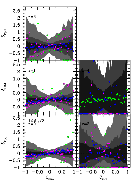
(b) $6\leq M_{12}<10$

Figure 29.— Autocorrelations between the major mergers at redshifts $z=0$, 1, 2, 3, 4, and 5 in the samples of $1\leq M_{12}<2$ (a) and $6\leq M_{12}<10$ (b).

Appendix E Number Distributions of Major Mergers

We determine the distribution of major merger frequency in each halo sample at $z=0$ to confirm our argument that void halos experience fewer major mergers, which may explain the deviations of the stochastic model prediction from $N$-body spin distributions. In Figure 30, we show the number of major mergers ($N_{\rm mm}$) per halo with masses $1\leq M_{12}<2$ (a) or $6\leq M_{12}<10$ (b). In the sample of $1\leq M_{12}<2$, the number difference between halos in different environments is not severe at higher redshift ($z\geq 2$), while, at lower redshifts, less dense samples clearly show fewer major mergers. However, more massive samples (b) show nearly negligible deviations from each other, demonstrating noticeable differences only at $z=0$. The peak number of the $N_{\rm mm}$ distribution is four, while it is three at higher redshifts ($z\geq 4$). Therefore, we conclude that the correlated random walk seen in void regions may be a joint effect of the major-to-major merger autocorrelation and the smaller number of major mergers in less dense regions. It is interesting to find that a significant fraction of halos in cluster regions do not experience a major merger event during their lifetime (5% of halos with $1\leq M_{12}<2$ and 1 % of halos with $6\leq M_{12}<10$). Also, the fraction of cluster halos needed to prohibit a major merger event after $z=1$ is significantly higher than that of halos in lower density regions.

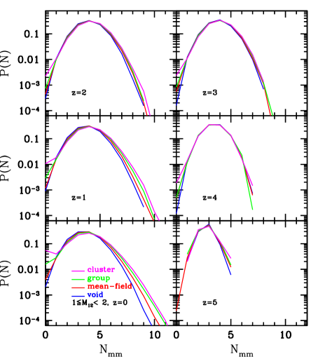
(a) $1\leq M_{12}<2$

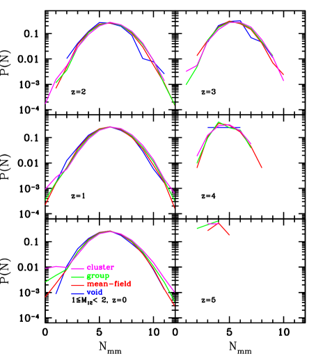
(b) $6\leq M_{12}<10$

Figure 30.— Number distributions of major mergers in the history of a halo until $z=0$, 1, 2, 3, 4, and 5 measured from the samples of $1\leq M_{12}<2$ (a) and $6\leq M_{12}<10$ (b).

Appendix F Statistical Properties in the Spin Distribution

In this section, we present the means and standard deviations of spin distributions from $N$-body simulations and random generations together with fitting results to a log-normal function with least $\chi^{2}$. See Tables 4 and 5. The mean value of the halo spin increases with local density and redshift. The difference between $N$-body and random simulations increases as local density decreases.

Table 4Spin Distributions for the Halo Mass Samples Used in Figures 11-13

		$N$-body Simulation			Random Generation
Halo Mass	Redshift	$\langle\log_{10}\lambda\rangle$	$\sigma_{\log_{10}\lambda}$	$\chi^{2}$/dof	$\langle\log_{10}\lambda\rangle$	$\sigma_{\log_{10}\lambda}$	$\chi^{2}$/dof
	0.0	-1.386	0.336	0.00118	-1.342	0.329	0.00140
$0.5\leq M_{12}<0.8$	0.5	-1.389	0.319	0.00076	-1.374	0.308	0.00071
	2.0	-1.434	0.290	0.00034	-1.429	0.289	0.00037
	0.0	-1.407	0.323	0.00068	-1.358	0.326	0.00107
$1\leq M_{12}<2$	0.5	-1.405	0.311	0.00037	-1.381	0.309	0.00059
	2.0	-1.450	0.291	0.00029	-1.427	0.294	0.00031
	0.0	-1.414	0.313	0.00038	-1.366	0.324	0.00080
$4\leq M_{12}<6$	0.5	-1.412	0.304	0.00028	-1.386	0.306	0.00049
	2.0	-1.474	0.291	0.00064	-1.439	0.296	0.00062
	0.0	-1.415	0.309	0.00027	-1.367	0.322	0.00090
$7\leq M_{12}<10$	0.5	-1.419	0.302	0.00028	-1.390	0.306	0.00061
	2.0	-1.488	0.292	0.00086	-1.446	0.304	0.00110

Note. — The mean and standard deviation of the halo spin from $N$-body simulation and random generation. Also, we list the least $\chi^{2}$ obtained during the log-normal fitting.

Table 5Spin Distributions for the Halo Samples Used in Figures 14-17

		$N$-body Simulation			Random Generation
Redshift	Environment	$\langle\log_{10}\lambda\rangle$	$\sigma_{\log_{10}\lambda}$	$\chi^{2}$/dof	$\langle\log_{10}\lambda\rangle$	$\sigma_{\log_{10}\lambda}$	$\chi^{2}$/dof
$1\leq M_{12}<2$
	void	-1.539	0.277	0.00108	-1.440	0.297	0.00083
$z=0$	mean-field	-1.486	0.284	0.00041	-1.424	0.297	0.00057
	group	-1.410	0.311	0.00050	-1.357	0.327	0.00083
	cluster	-1.287	0.375	0.00238	-1.287	0.374	0.00130
	void	-1.544	0.273	0.00125	-1.432	0.294	0.00059
$z=1$	mean-field	-1.489	0.279	0.00053	-1.435	0.291	0.00055
	group	-1.412	0.293	0.00028	-1.391	0.299	0.00050
	cluster	-1.317	0.320	0.00058	-1.332	0.320	0.00065
	void	-1.564	0.272	0.00168	-1.457	0.290	0.00081
$z=2$	mean-field	-1.522	0.277	0.00069	-1.461	0.289	0.00043
	group	-1.454	0.285	0.00036	-1.424	0.294	0.00038
	cluster	-1.369	0.298	0.00026	-1.367	0.303	0.00043
$6\leq M_{12}<10$
	void	-1.574	0.268	0.01237	-1.529	0.319	0.01626
$z=0$	mean-field	-1.516	0.285	0.00112	-1.459	0.318	0.00145
	group	-1.423	0.300	0.00036	-1.378	0.315	0.00073
	cluster	-1.335	0.328	0.00072	-1.290	0.347	0.00101
	void	-1.635	0.274	0.03620	-1.585	0.305	0.02587
$z=1$	mean-field	-1.549	0.280	0.00339	-1.504	0.296	0.00257
	group	-1.447	0.288	0.00074	-1.421	0.294	0.00067
	cluster	-1.360	0.298	0.00062	-1.335	0.301	0.00090
	void	-1.679	0.283	0.10107	-1.589	0.349	0.10899
$z=2$	mean-field	-1.613	0.270	0.01070	-1.537	0.317	0.00637
	group	-1.520	0.281	0.00169	-1.472	0.302	0.00155
	cluster	-1.435	0.293	0.00154	-1.384	0.306	0.00190

Note. — Same as Table 4.

Appendix G Effect of MERGING MODEL on Spin Distribution

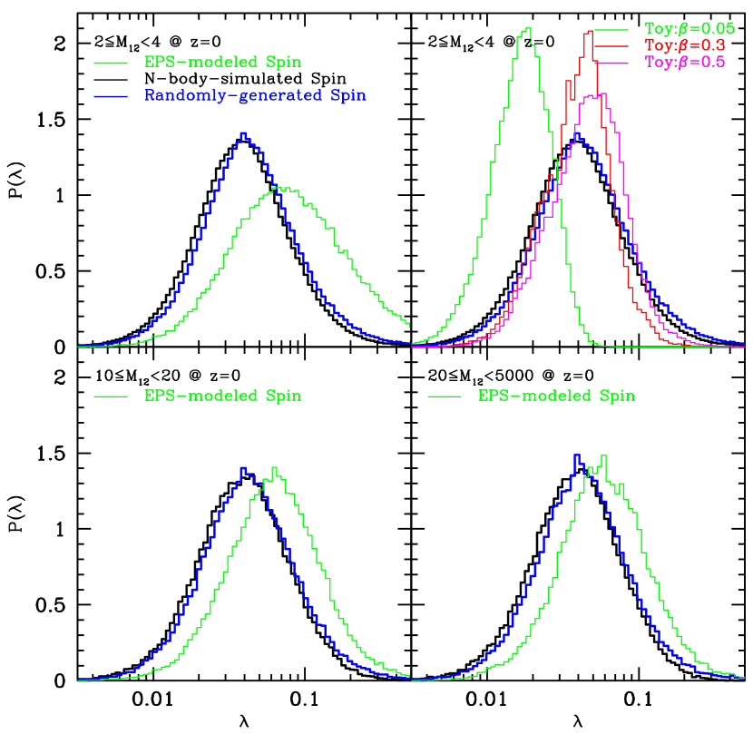
Figure 31.— Spin distributions from the EPS model of the spherical top-hat collapse (Lacey & Cole, 1993); top-left and bottom row panels) and from the toy model with various $\beta$’s (top-right panel) at $z=0$.

In this section, we demonstrate the effects of major merging and accretion on the spin distributions in a simple toy merging model. The mass increase is parameterized as

$$\beta\equiv{\Delta M\over M},$$ (G1)

where $\beta$ is set constant over the halo mass evolution. The number of time steps is, therefore, determined from the input value of $\beta$ for given initial and final halo masses. In the top right panel of Figure 31, we observe that a higher value of $\beta$ makes the spin distribution move to a higher $\lambda$. However, the actual mass growth is a spectrum of $\Delta M/M$ with a certain probability distribution and this shapes the spin distributions found in simulations.

Next, we test whether the mass accretion histories derived from the classical extended Press-Schechter (EPS) formalism may give a probability distribution of $\Delta M/M$ comparable to the simulated ones. We generate merging trees according to the EPS merging model of the spherical top-hat collapse (Lacey & Cole, 1993). The conditional probability of a progenitor to have a density contrast of $\delta_{c}(t_{1})$ at the smoothing scale of $M_{1}$ is (Jiang & van den Bosch, 2014)

$$f_{\rm SC}(S_{1},\omega_{1}|S_{0},\omega_{0})={1\over\sqrt{2\pi}}{\Delta\omega\over\Delta S^{3/2}}e^{-{\Delta\omega^{2}\over 2\Delta S}},$$ (G2)

where $\Delta S\equiv S_{1}-S_{0}$, $S_{i}\equiv\sigma^{2}(M_{i})$, $\Delta\omega\equiv\omega_{1}-\omega_{0}$, and $\omega_{i}\equiv\delta_{c}(t_{i})$ for $t_{0}>t_{1}$. Using this equation, we generate the 100,000 random mass-merging trees and follow the stochastic spin changes for several halo mass samples (see Fig. 31) at $z=0$. In the figure, the EPS model predicts that the spin distributions will shift to higher values of $\lambda$, but this tendency is smaller for larger mass samples. This means that the spectrum of merger rates from the least accretion to most-massive major merger modeled by the classical EPS model may be different from $N$-body results. Thus, the results suggest that it would be interesting to test whether other variant, and certainly more advanced, EPS models that have been well known to provide halo mass functions consistent with simulations may also produce spin distributions similar to those from $N$-body simulation by adopting this stochastic modeling.

References

- Ahn et al. (2014) Ahn, J., Kim, J., Shin, J., Kim, S. S., & Choi, Y.-Y. 2014, Journal of Korean Astronomical Society, 47, 77