Analyzing Linear Communication Networks using the Ribosome Flow Model

Abstract

The Ribosome Flow Model (RFM) describes the unidirectional movement of interacting particles along a one-dimensional chain of sites. As a site becomes fuller, the effective entry rate into this site decreases. The RFM has been used to model and analyze mRNA translation, a biological process in which ribosomes (the particles) move along the mRNA molecule (the chain), and decode the genetic information into proteins.

Here we propose the RFM as an analytical framework for modeling and analyzing linear communication networks. In this context, the moving particles are data-packets, the chain of sites is a one dimensional set of ordered buffers, and the decreasing entry rate to a fuller buffer represents a kind of decentralized backpressure flow control. For an RFM with homogeneous link capacities, we provide closed-form expressions for important network metrics including the throughput and end-to-end delay. We use these results to analyze the hop length and the transmission probability (in a contention access mode) that minimize the end-to-end delay in a multihop linear network, and provide closed-form expressions for the optimal parameter values.

I Introduction

The inflation of wireless devices and the dramatic increase in demand for real-time applications has led to a growing interest in the analysis and design of mobile ad hoc networks (MANETs). Important features of MANETs include: nodes may operate as clients and as routers; flow control is decentralized; and the communication infrastructure between the nodes changes dynamically on the basis of network connectivity. The end-to-end features of such networks depend on the intricate correlations between the different flows in the system. The rigorous analysis of basic network characteristics, such as end-to-end delay, buffer utilization, and throughput, is a non-trivial challenge

Wireless networks have been analyzed using different tools including information theory [1] and queuing theory [2, 3]. However, these often use simplified assumptions and yield approximate results when characterizing the network throughput and delay performances. For example, large scale $2D$ networks have been studied based on Kleinrock’s Independence Assumption [4]. According to this assumption, traffic correlations between different flows can be ignored and the effect on delay performance is negligible, subject to sufficient traffic mixing and moderate-to-heavy traffic loads (see e.g., [5]). However, recent studies suggest that this assumption does not hold in various real-world communication networks [2]. Ad-hoc networks have also been modeled as a network of Jackson queues [6, 7]. This is a stochastic model that assumes independent M/M/1 queues along the network. The service times are exponentially distributed and are mutually independent. As such, the average number of data-packets in each node is determined independently from the node’s neighbors and thus the interaction between adjacent nodes is neglected.

Andrews et al. [8] point out that standard analysis tools may not be adequate for MANETs. They suggest several other tools, including non-equilibrium statistical mechanics. They state that: “In particular, the microscopic theories of vehicular traffic are promising since they do not treat vehicle flows as compressible fluids but explicitly focus on the dynamics of the individual vehicle. In other words, the theories treat the vehicular network as a system of interacting particles driven far from equilibrium, enabling the study of the dynamics of more general non-equilibrium systems-such as MANETs.”

An interesting paper [9] (see also [10, 11]) has suggested using the Totally Asymmetric Simple Exclusion Process (TASEP) [12] to model and analyze ad hoc networks. TASEP is a stochastic model for particles that move along some kind of “tracks” or “trails”. A lattice of sites models the tracks. Each site may either be free or contain a single particle. Particles hop, with some probability, from one site to the consecutive one, but only if the target site is free (hence the term simple exclusion). This models particles that have volume and cannot overtake one another. In this way, the model captures the interaction between the particles. The term totally asymmetric is used to indicate that motion is unidirectional.

TASEP and its variants are regarded as a paradigmatic model in non-equilibrium statistical mechanics, and have been used to model and analyze numerous natural and artificial multiagent systems, including traffic flow, molecular motors, mRNA translation and more [13, 14, 12]. For example, in the context of traffic flow, the particles [lattice] represent cars [the road].

Recently, Reuveni et al. [15] studied a deterministic non-linear model, called the ribosome flow model (RFM), that can also be derived by mean-field approximation of TASEP. Although nonlinear, the RFM is amenable to mathematical analysis using various tools including the analytical theory of continued fractions [16, 17], monotone systems theory [18, 19], contraction theory [20], convex optimization theory [21], and matrix theory [22].

We propose the RFM as a theoretical framework for linear communication networks. In this context, the moving particles are data-packets and the chain of sites is a one dimensional set of ordered buffers. For the RFM with homogeneous link capacities, we provide closed-form expressions for important features including: steady-state buffer occupancy, network throughput, and end-to-end delay. We use these results to provide closed-form expressions for the hop length and the transmission probability that minimize the end-to-end delay in ad-hoc multihop linear networks.

The remainder of this paper is organized as follows. Section II reviews the RFM. Section III explains how the RFM can be used to model a linear communication network. Section IV presents the main results. Section V describes two applications of these results to a multihop network. Section VI concludes and describes possible directions for future research. To streamline the presentation, all the proofs are placed in the Appendix.

II Ribosome Flow Model

The RFM is a set of $n$ nonlinear first-order ordinary differential equations (ODEs):

$$\dot{x}_{1} =\lambda_{0}(1-x_{1})-\lambda_{1}x_{1}(1-x_{2})$$

$$\dot{x}_{2} =\lambda_{1}x_{1}(1-x_{2})-\lambda_{2}x_{2}(1-x_{3})$$ (1)

$$\vdots$$

$$\dot{x}_{n} =\lambda_{n-1}x_{n-1}(1-x_{n})-\lambda_{n}x_{n}.$$

This is a compartmental model [23], consisting of $n$ compartments (or sites) ordered along a linear 1D chain. Each site may contain some material. (In the case studied here, each site is a buffer that contains data-packets of fixed length.) The state-variable $x_{i}(t)$, $i\in\{1,\dots,n\}$, represents the occupancy level of site $i$ at time $t$. The occupancy levels are normalized so that $x_{i}(t)\in[0,1]$ for all $t\geq 0$, with $x_{i}(t)=0$ [$x_{i}(t)=1$] representing that site $i$ is completely empty [full] at time $t$. Site $1$ is fed by a source with entry rate $\lambda_{0}>0$. Material flow from site $i$ to site $i+1$ depends on a elongation rate $\lambda_{i}>0$. The material exits at the end of the chain, that is, from buffer $n$ with exit rate $\lambda_{n}>0$.

To explain the equations of this model, consider the equation for $\dot{x}_{1}$, i.e., the rate of change in occupancy level at site $1$. The term $\lambda_{0}(1-x_{1})$ is the transition rate into the chain: as $x_{1}$ increases this rate decreases and, in particular, when $x_{1}=1$ (i.e., buffer $1$ is completely full) this rate becomes zero. The term $\lambda_{1}x_{1}(1-x_{2})$ is the transition rate of material from site $1$ to the consecutive site $2$. This is proportional to the occupancy level at site $1$, and also to $(1-x_{2})$. In particular, when $x_{2}=1$ this becomes zero. Thus, as site $2$ becomes fuller the flow from site $1$ to site $2$ decreases. In this way, the RFM encapsulates both the simple exclusion principle and the unidirectional movement of TASEP. The exit rate from the last site is $R(t):=\lambda_{n}x_{n}(t)$. (In the biological context, this represents the protein production rate.)

The state space of the RFM is the $n$-dimensional unit cube $C^{n}:=[0,1]^{n}$. Let $\operatorname{{\mathrm{i}nt}}(C^{n})$ denote the interior of $C^{n}$, and let $x(t,a)$ denote the solution of the RFM at time $t$ for the initial condition $x(0)=a$.

Proposition 1

[18] The RFM admits a unique equilibrium point $e=e(\lambda_{0},\dots,\lambda_{n})\in\operatorname{{\mathrm{i}nt}}(C^{n})$, and for any $a\in C^{n}$, $x(t,a)\in\operatorname{{\mathrm{i}nt}}(C^{n})$ for all $t>0$, and $\lim_{t\to\infty}x(t,x_{0})=e.$

This means that every trajectory of the RFM converges to a steady-state that depends on the rates $\lambda_{0},\dots,\lambda_{n}$. In particular, $R(t)$ converges to the steady-state exit rate $R:=\lambda_{n}e_{n}$.

The simulation results reported in [15] show that RFM and TASEP yield similar predictions of steady-state rates. However, recent research results on the RFM suggest that expressions for important quantities are considerably simpler than the corresponding expressions in TASEP.

Several recent papers analyzed the RFM. In the particular case where $\lambda_{1}=\cdots=\lambda_{n}:=\lambda_{c},$ with $\lambda_{c}$ denoting the common value, the RFM is called the Homogeneous Ribosome Flow Model (HRFM). This model includes only two parameters $\lambda_{0}$ and $\lambda_{c}$, so its analysis becomes more tractable [16]. The HRFM with an infinitely-long chain, (i.e. with $n\to\infty$) was considered in [17]. There, a simple closed-form expression for $e_{\infty}:=\lim_{n\to\infty}e_{n}$ was derived, as well as explicit bounds for $|e_{\infty}-e_{n}|$ for all $n\geq 2$. A closed-loop RFM (representing mRNA circularization) has been studied in [19]. It has been shown that the closed-loop system admits a unique globally asymptotically stable equilibrium point. Ref. [20] has shown that when the rates $\lambda_{i}$ are periodic functions of time, with a common period $T$, then (II) admits a unique periodic solution $p(t)$, with period $T$, and $x(t,x_{0})\to p(t)$ for every initial condition $x_{0}\in C^{n}$. In other words, the RFM entrains to periodic excitations in the rates. Ref. [21] has shown that the steady-state exit rate $R=R(\lambda_{0},\dots,\lambda_{n})$ is a strictly concave function of $\lambda_{0},\dots,\lambda_{n}$ on $\mathbb{R}^{n+1}_{++}$. This means that the problem of maximizing the steady-state exit rate, under an affine constraint on the rates, is a convex optimization problem.

III Modeling Linear Communication Networks using the RFM

Fig. 1 illustrates the general block diagram of a linear communication network with multiple relay nodes modeled using the RFM. Here the material flowing is data packets, each site corresponds to a communication node that contains a buffer, and $x_{i}(t)$ is the (normalized) occupancy of buffer $i$ at time $t$. The parameter $\lambda_{i}>0$ is the capacity of the link from node $i$ to node $i+1$. The network throughput at time $t$ is $R(t)$. The equation $\dot{x}_{i}=\lambda_{i-1}x_{i-1}(1-x_{i})-\lambda_{i}x_{i}(1-x_{i+1})$ represents a decentralized flow control algorithm, as the flow through buffer $i$ depends on the occupancy at buffers $i-1$ ,$i$, and $i+1$ only.

Prop. 1 means that for any set of strictly positive link capacities the flow control algorithm is stable in a strong sense, as the dynamics keeps every buffer from overflow or underflow at all time $t$ (QoS flows are one example where buffer overflow must be avoided). Furthermore, the network always converges to a steady state in which the occupancy of buffer $i$ is $e_{i}\in(0,1)$. Note that $e_{i}$ may also be interpreted as the probability that site $i$ is occupied at steady-state.

Recall that the backpressure algorithm (see, e.g., [24, 25, 26, 27, 28]) schedules packets from node $i$ to node $i+1$ based on the differential backlog $\max\{0,x_{i}-x_{i+1}\}$. As $x_{i}$ increases and $x_{i+1}$ decreases, the effective flow rate increases. This also happens in the RFM, as the flow rate is $\lambda_{i}x_{i}(1-x_{i+1})$.

Note that TASEP is a stochastic, discrete-time, asynchronous model, whereas the RFM is a deterministic, continuous-time, synchronous model. Indeed, in the RFM all the $x_{i}$s are updated synchronously. Conceptually, the RFM [TASEP] is more suitable for modeling access protocols like slotted-ALOHA or CDMA [TDMA] where the nodes [do not] transmit at the same time.

In the context of communication networks, TASEP corresponds to a chain of buffers, where each buffer can either contain a packet or not. The RFM provides a more flexible framework, as the buffer level $x_{i}$ takes values in $[0,1]$, so the buffer can be either empty ($x_{i}=0$), full ($x_{i}=1$), half full ($x_{i}=1/2$), and so on. As shown in Section IV, analysis of the RFM leads to simpler expressions than those known for TASEP. Nevertheless, below we also simulate the time-averaged steady-state behavior of TASEP and show that the results agree well with the analytical formulas derived for the RFM.

Figure 1: Linear communication network with $n$ relay-nodes modeled using the RFM. SRC [DST] represents the source [destination] node. The circles represent the relays. State-variable $x_{i}(t)\in[0,1]$ is the normalized number of data-packets at buffer $i$ at time $t$. The capacity of the link from site $i$ to site $i+1$ is $\lambda_{i}$. The throughput at time $t$ is $R(t)=\lambda_{n}x_{n}(t)$.

IV Analysis of Linear Communication Networks using the RFM

In this section, we analyze properties of the RFM that are relevant for communication networks. We consider the special case where all the link capacities are equal, i.e. $\lambda_{0}=\cdots=\lambda_{n}:=\lambda_{c}$. We refer to this case as the totally homogeneous RFM (THRFM).

Proposition 2

Consider the THRFM with $n$ sites. The steady-state occupancy level at site $i$ is

$$e_{i}=\frac{1}{2}+\frac{1}{2}\tan\left(\frac{\pi}{n+3}\right)\cot\left(\frac{(i+1)\pi}{n+3}\right),\quad i=1,\dots,n.$$ (2)

The steady-state throughput is

$$R=\frac{\lambda_{c}}{4\cos^{2}(\frac{\pi}{n+3})}.$$ (3)

The steady-state delay experienced by a data-packet at node $i$ is

$$D_{i}=\frac{2}{\lambda_{c}}\cos^{2}\left(\frac{\pi}{n+3}\right)\left(1+\tan(\frac{\pi}{n+3})\cot(\frac{(i+1)\pi}{n+3})\right),$$ (4)

and the end-to-end delay is

$$D_{e2e}:=\sum_{i=1}^{n}D_{i}=\frac{2n}{\lambda_{c}}\cos^{2}\left(\frac{\pi}{n+3}\right).$$ (5)

Eq. (2) implies that the steady-state buffer occupancies are independent of the homogeneous link capacity $\lambda_{c}$ (but $\lambda_{c}$ does control the convergence rate to the steady-state). Combining (2) with the identity $\cot(x)=-\cot(\pi-x)$ implies the symmetry relation $e_{i}-\frac{1}{2}=\frac{1}{2}-e_{n+1-i}$, and this gives

$$\sum_{i=1}^{n}e_{i}=n/2.$$ (6)

This implies that for $n$ odd, $e_{(n+1)/2}=1/2$. Eq. (2) also implies that $e_{1}>\cdots>e_{n}$. This means that at steady-state, much of the queuing occurs closer to the source node, and preference is given to nodes closer to the destination node. Indeed, it was suggested that a scheduling algorithm giving preference to serving links closer to the destination node achieves optimal end-to-end buffer usage in linear networks [29].

Fig. 2 depicts the $e_{i}$s for a network with $n=19$ nodes. It may be seen that $e_{i}$ decreases with $i$. Note also the symmetry around $e_{10}=1/2$. For example, $e_{8}-\frac{1}{2}=\frac{1}{2}-e_{12}$. Fig. 2 also depicts empirical occupancy levels obtained via simulation of TASEP with $n=19$ nodes.

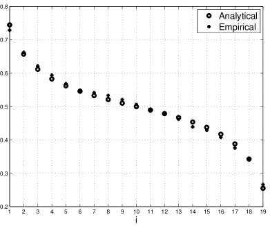
Figure 2: Analytical (O) and empirical (+) steady-state occupancy level $e_{i}$ as a function of $i=1,\dots,19$, in a THRFM with $n=19$ nodes.

Eq. (3) implies that: (1) the steady-state throughput $R$ is proportional to the homogeneous link capacity $\lambda_{c}$; (2) $R$ is upper-bounded by $\lambda_{c}/2$ for all $n$; and (3) $R$ decreases with the network length $n$, with $\lim_{n\to\infty}R=\lambda_{c}/4$ (see Fig. 3).

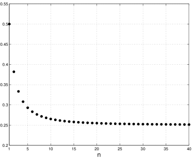
Figure 3: Throughput $R$ for link capacity $\lambda_{c}=1$ as a function of $n$.

Eq. (4) implies that $D_{1}>\cdots>D_{n}$, as the steady-state delay experienced by a data-packet at node $i$ is proportional to the occupancy level at that node. The end-to-end delay $D_{e2e}$ is inversely proportional to the link capacity $\lambda_{c}$, and increases more or less linearly with the network length $n$. In particular, $D_{e2e}\approx{2n}/{\lambda_{c}}$ for large values of $n$. Fig. 4 depicts $D_{e2e}$ as a function of $\lambda_{c}$ for a THRFM with $n=19$. It also shows the empirical values of $D_{e2e}$ obtained via simulating TASEP and averaging the end-to-end delays of data-packets (after discarding the first $350,000$ cycles).

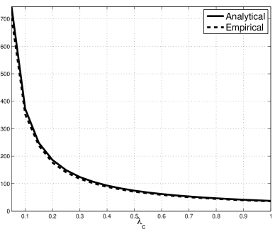
Figure 4: Steady-state end-to-end delay $D_{e2e}$ as a function of the link capacity $\lambda_{c}$ in a network with $n=19$ nodes.

V Application to Multihop Networks

Ad-hoc multihop networks and their military and civilian applications are attracting considerable interest, yet there remain significant theoretical challenges in the performance analysis of these networks [30, 31, 8], and thus in their systematic design. The decentralized, multiagent network structure and the possibility for multihop routing make the analysis of fundamental communication metrics, including throughput, latency and capacity quite challenging. In multihop networks, data-packets may be routed over many short hops or over a smaller number of long hops. An important research topic is determining various parameters, e.g. the hop length, that optimize some performance metric, e.g. minimize the end-to-end delay. (Of course, in general there could be additional factors impacting the decision between short and long hops [32].) In this section we show how to use the analysis results on the THRFM described above to systematically address this type of optimization problems.

We assume that all the nodes in the network use the same channel. The nodes are equally spaced along the communication system, with a separation $\ell$ between any two adjacent nodes. Attenuation in the channel is modeled as the product of a Rayleigh fading component and a large-scale path loss component with exponent $\gamma$. The channel noise is taken to be additive white Gaussian noise (AWGN) with power spectral density $N_{0}$. We define the transmission from node $i$ to node $i+1$ to be successful if the (instantaneous) signal-to-interference-and-noise ratio (SINR) at node $i+1$ is greater than a predetermined threshold $\Theta$. The probability of a successful transmission is thus $p_{s}:=\text{Pr}(\text{SINR}>\Theta)$.

V-1 Optimal Hop Length at SNR Limit Regime

Consider an ad-hoc multihop linear network where the main effect on a successful transmission is the channel attenuation and noise. This happens, for example, when the nodes are relatively far so that the effect of the spatial reuse is negligible relative to the channel noise. In this regime,

$$p_{s}=\text{Pr}(\text{SNR}>\Theta)=\exp(-\Theta N_{0}l^{\gamma}).$$ (7)

We model this using the THRFM with link capacities $\lambda_{c}=rp_{s}$, where $r>0$. For simplicity, we take $r=1$. The end-to-end delay in the THRFM given in (5) then becomes

$$D_{e2e}=2n\exp(\Theta N_{0}l^{\gamma})\cos^{2}\left(\frac{\pi}{n+3}\right).$$ (8)

The closed-form expression for $D_{e2e}$ allows us to address various optimization problems. For example, consider the problem of finding the hop length that minimizes the end-to-end delay. Let $ml$ denote a hop of $m$ steps of unit length $l$. Replacing $l$ with $ml$ and $n$ with $n/m$ in (8) yields

$$D_{e2e}=\frac{2n}{m}\exp(\Theta N_{0}(ml)^{\gamma})\cos^{2}\left(\frac{\pi}{(n/m)+3}\right).$$ (9)

In particular, for $n/m\gg 1$,

$$D_{e2e}\approx\bar{D}_{e2e}:=\frac{2n}{m}\exp(\Theta N_{0}(ml)^{\gamma}).$$ (10)

This expression shows that $m$ affects $D_{e2e}$ in two different ways. On the one-hand, increasing $m$ decreases the total length of the chain and thus decreases the delay. On the other-hand, increasing $m$ increases the separation between the communicating nodes. This decreases the probability of a successful transmission thus increasing the delay.

Proposition 3

The hop length that minimizes the end-to-end delay $\bar{D}_{e2e}$ in the SNR limit regime is either $\lceil m^{*}\rceil$ or $\lfloor m^{*}\rfloor$, where

$$m^{*}:=\frac{1}{l}\left(\frac{1}{\gamma\Theta N_{0}}\right)^{{1}/\gamma},$$ (11)

and for this value, the optimal end-to-end delay is

$$\bar{D}_{e2e}^{*}={2}nl\left(\gamma\Theta N_{0}\right)^{{1}/\gamma}\exp(1/\gamma).$$

Eq. (11) implies that $m^{*}$ is monotonically decreasing with $\Theta$ and $N_{0}$. This is reasonable, as an increase in any of these parameters decreases the effective SNR at the receiving node, which in turn decreases the probability of a successful transmission. This can be compensated by decreasing the hop length. Fig. 5 depicts the analytical and empirical values of $m^{*}$ as a function of $\Theta$ and $\gamma$ for $\ell=1$ and $N_{0}=-50$ dBW/Hz. The empirical values were obtained by simulating several TASEPs, each one with $200/m$ sites and with an exponentially distributed next time to hop with parameter $\lambda_{c}=p_{s}$ as given in (7), but with $\ell$ replaced by $m\ell$.

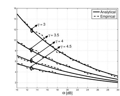
Figure 5: Optimal hop length $m^{*}$ as a function of the SNR threshold $\Theta$ and the path loss exponent $\gamma$ for a network with $n=200$ nodes.

V-2 Optimal Transmission Probability at SIR Limit Regime

Consider now an ad-hoc multihop wireless network where the main effect on a successful transmission is the transmission interference. Let $q$ denote the contention probability, i.e. the probability that a node transmits at each time slot. In this case,

$$p_{s}\approx\exp({-qc}/{2}),$$ (12)

where $c:=\frac{\pi\Theta^{\frac{1}{\gamma}}}{\sqrt{\gamma/2}}-1$ (see [33]).

A natural question is how to determine the contention probability that minimizes $D_{e2e}$. To address this, we model this scenario as a THRFM with $\lambda_{c}=qp_{s}$. Substituting this in (5) yields

$$D_{e2e}=(v/q)\exp(qc/2),$$ (13)

where $v:=2n\cos^{2}\left(\frac{\pi}{n+3}\right)$. This expression shows that $q$ affects $D_{e2e}$ in two different ways. On the one-hand, increasing $q$ increases the link capacity and thus decreases the delay. On the other-hand, increasing $q$ increases the interference. This decreases the probability of a successful transmission thus increasing the delay.

Proposition 4

The contention probability that minimizes the end-to-end delay in the SIR limit regime is

$$q^{*}=\min\{1,2/c\}.$$ (14)

Fig. 6 depicts the analytical and empirical optimal contention probability $q^{*}$ as a function of $\Theta$ and $\gamma$. Note that $q^{*}$ is inversely proportional to both $\Theta$ and to $\gamma$.

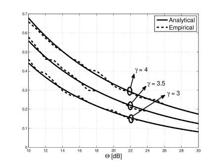
Figure 6: Optimal transmission probability $q^{*}$ as a function of the threshold $\Theta$ and the path loss exponent $\gamma$.

VI Discussion

TASEP is an important model in non-equilibrium statistical mechanics that has been used to study numerous biological and artificial multiagent systems including multihop wireless networks [9, 10, 11]. The RFM is a “deterministic substitute” of TASEP that is highly amenable to mathematical analysis. In this paper, we proposed the RFM as a new theoretical framework for modeling and analyzing linear communication networks. This has several advantages. The dynamics of the RFM guarantees that the buffer levels do not overflow or underflow for all time $t$, and converge to a unique steady-state level. For the particular case of the THRFM, another important advantage is that simple closed-form expressions for important network metrics such as the steady-state throughput and end-to-end-delay exist. These expressions can be used to select optimal parameters, for example, the optimal hop length in a multihop network.

For the more general case of an RFM with non-homogeneous rates closed-form expressions for the network metrics are not known. However, they can be easily computed in an efficient and numerically stable way. Indeed, it has been shown in [21] that the $(n+2)\times(n+2)$ matrix

$$\small A:=\begin{bmatrix}0&\lambda_{0}^{-1/2}&0&0&\dots&0&0\\ \lambda_{0}^{-1/2}&0&\lambda_{1}^{-1/2}&0&\dots&0&0\\ 0&\lambda_{1}^{-1/2}&0&\lambda_{2}^{-1/2}&\dots&0&0\\ &&&\vdots\\ 0&0&0&\dots&\lambda_{n-1}^{-1/2}&0&\lambda_{n}^{-1/2}\\ 0&0&0&\dots&0&\lambda_{n}^{-1/2}&0\end{bmatrix}$$ (15)

has real and distinct eigenvalues: $\zeta_{1}<\zeta_{2}<\dots<\zeta_{n+2},$ and that the steady-state throughput in the RFM is $R=\left(\zeta_{n+2}\right)^{-2}$. This means that $R$, and then every other steady-state metric, can be determined using numerical algorithms for calculating the eigenvalues of symmetric (tridiagonal) matrices.

The link capacities in a communication network must often be constrained, e.g. to reduce interference or because of energy constraints [34]. A natural question is how to maximize the throughput subject to a constraint on the capacities. In the linear communication network modeled using the RFM, this leads to the following optimization problem:

Problem 1

Fix $b,w_{0},w_{1},\dots,w_{n}>0$. Maximize $R=R(\lambda_{0},\dots,\lambda_{n})$, with respect to its parameters $\lambda_{0},\dots,\lambda_{n}$, subject to the constraints:

$$\sum_{i=0}^{n}w_{i}\lambda_{i} \leq b,$$ (16)

$$\lambda_{0},\dots,\lambda_{n} \geq 0.$$

The values $w_{i}$ can be used to provide different weighting to the different link capacities. It has been shown in [21] that $R$ is a strictly concave function of the $\lambda_{i}$s, and since the constraint on the rates is affine, Problem 1 is a convex optimization problem. Thus, the solution $\lambda_{i}^{*}$, $i=0,\dots,n$, is unique and can be found using efficient numerical algorithms that scale well with $n$.

Fig. 7 depicts the optimal link capacities $\lambda_{i}^{*}$, $i=0,\dots,9$, for a communication network with $9$ relay nodes and the constraint (16) with $w_{0}=\dots=w_{n}=b=1$. It may be seen that the $\lambda_{i}^{*}$s are symmetric, i.e. $\lambda_{i}^{*}=\lambda_{9-i}^{*}$, and that they increase towards the center of the network. In other words, the capacities near the center of the network have a higher effect on the throughput than those near the ends of the network.

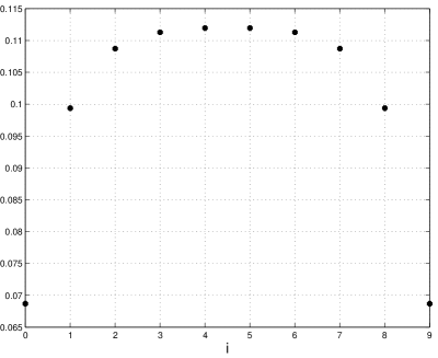
Figure 7: Optimal link capacities $\lambda_{i}^{*}$ as a function of $i$ for a linear communication network with $n=9$ nodes.

Another interesting research topic is to model and analyze more complex network topologies, comprising of multiple flows that share common nodes, using a set of interconnected RFMs.

Appendix: Proofs

Proof of Prop. 2. It has been shown in [16] that for an HRFM with $m$ sites and $\lambda_{0}\to\infty$ the equilibrium point $e=\begin{bmatrix}e_{1},\dots,e_{m}\end{bmatrix}^{\prime}$ satisfies $e_{i}=\frac{d_{i}}{2\cos(\frac{\pi}{m+2})}$, $i=1,\dots,m$, where $d_{i}:=\cos(\frac{\pi}{m+2})+\sin(\frac{\pi}{m+2})\cot(\frac{i\pi}{m+2})$. In particular, $e_{1}=1$. Since $\lambda_{1}=\dots=\lambda_{n}=\lambda_{c}$, (II) implies that the steady-state satisfies $\begin{bmatrix}e_{1}&e_{2}&\cdots&e_{m}\end{bmatrix}=\begin{bmatrix}1&\tilde{e}_{1}&\cdots&\tilde{e}_{m-1}\end{bmatrix}$, where $\begin{bmatrix}\tilde{e}_{1}&\cdots&\tilde{e}_{m-1}\end{bmatrix}$ is the equilibrium of a THRFM with dimension $m-1$. Taking $m=n+1$ yields (2). At steady-state, the exit rate is $R=\lambda_{n}e_{n}=\lambda_{c}e_{n}$, and this is equal to the rate of packet flow across each node. Combining this with (2) yields (3). By Little’s Theorem [6], the delay at node $i$ at steady-state is $D_{i}=e_{i}/R$. Combining this with (3) and (2) yields (4). The end-to-end delay is $\sum_{i=1}^{n}D_{i}=(1/R)\sum_{i=1}^{n}e_{i}$, and using (6) and (3) yields (5). ∎

Proof of Prop. 3. Differentiating $\bar{D}_{e2e}$ with respect to $m$ yields $\frac{\partial}{\partial m}\bar{D}_{e2e}=\frac{2n}{m^{2}}\exp(N_{0}\Theta(lm)^{\gamma})\left(\gamma N_{0}\Theta(lm)^{\gamma}-1\right),$ and $\frac{\partial^{2}}{\partial m^{2}}\bar{D}_{e2e}=\frac{2n}{m^{3}}\exp(z)(\gamma^{2}z^{2}+z\gamma(\gamma-3)+2),$ where $z:=\Theta N_{0}(ml)^{\gamma}$. It is straightforward to verify that $\frac{\partial^{2}}{\partial m^{2}}\bar{D}_{e2e}>0$ for all $m>0$ and $\gamma\geq 1$, thus for all practical cases $\bar{D}_{e2e}$ is a strictly convex function of $m$, and the unique global minimum $m^{*}$ can be found by equating $\frac{\partial}{\partial m}\bar{D}_{e2e}$ to zero, which yields (11) (of course, the relevant value is either $\lceil m^{*}\rceil$ or $\lfloor m^{*}\rfloor$, as the hop length must be an integer). Substituting $m^{*}$ in (10) completes the proof. ∎

Proof of Prop. 4. Differentiating (13) yields $\frac{\partial}{\partial q}D_{e2e}=v\exp(cq/2)\frac{cq-2}{2q^{2}},$ and $\frac{\partial^{2}}{\partial q^{2}}D_{e2e}=v\exp(cq/2)\frac{f(cq)}{4q^{3}},$ where $f(z):=z^{2}-4z+8$. Since $v>0$ and $f(z)>0$ for all $z$, it follows that $\frac{\partial^{2}}{\partial q^{2}}D_{e2e}>0$ for all $q>0$, so $D_{e2e}$ is a strictly convex function of $q$, and the unique global minimum $q^{*}$ can be found by equating $\frac{\partial}{\partial q}D_{e2e}$ to zero. This yields $q^{*}=2/c$. If $c\geq 2$ then $q^{*}=2/c\leq 1$, so this is a valid minimizer (recall that $q\in(0,1]$). If $c<2$ then $2/c>1$, so the valid minimum is $q^{*}=1$. ∎

References

- [1] A. E. Gamal and Y.-H. Kim, Network Information Theory. Cambridge University Press, 2011.
- [2] M. Xie and M. Haenggi, “Towards an end-to-end delay analysis of wireless multihop networks,” Ad Hoc Networks, vol. 7, pp. 849–861, 2009.
- [3] N. Bisnik and A. A. Abouzeid, “Queuing network models for delay analysis of multihop wireless ad hoc networks,” Ad Hoc Networks, vol. 7, no. 1, pp. 79–97, 2009.
- [4] R. Nelson and L. Kleinrock, “Spatial TDMA: A collision-free multihop channel access protocol,” IEEE Trans. Communications, vol. 33, pp. 934–944, 1985.
- [5] T. Jun and C. Julien, “Delay analysis for symmetric nodes in mobile ad hoc networks,” in Proc. 4th ACM Workshop on Performance Monitoring and Measurement of Heterogeneous Wireless and Wired Networks, 2009, pp. 191–200.
- [6] L. Kleinrock, Queueing Systems Theory. Wiley-Interscience, 1975, vol. 1.
- [7] J. R. Jackson, “Networks of waiting lines,” Operations Research, vol. 5, no. 4, pp. 518–521, 1957.
- [8] J. Andrews, S. Shakkottai, R. Heath, N. Jindal, M. Haenggi, R. Berry, D. Guo, M. Neely, S. Weber, S. Jafar, and A. Yener, “Rethinking information theory for mobile ad hoc networks,” IEEE Commun. Mag., vol. 46, no. 12, pp. 94–101, December 2008.
- [9] S. Srinivasa and M. Haenggi, “A statistical mechanics-based framework to analyze ad hoc networks with random access,” IEEE Trans. Mobile Comput., vol. 11, pp. 618–630, 2012.
- [10] M. Liu, S. Zhao, J. Yang, and Z. Li, “Towards a model for information traffic flow in wireless networks,” in Proc. 3rd Int. Conf. Computer and Electrical Engineering (ICCEE 2010), 2012.
- [11] S. Srinivasa and M. Haenggi, “The TASEP: A statistical mechanics tool to study the performance of wireless line networks,” in Proc. th Int. Conf. Computer Communications and Networks (ICCCN2010), Zurich, Switzerland, 2010, pp. 1–6.
- [12] A. Schadschneider, D. Chowdhury, and K. Nishinari, Stochastic Transport in Complex Systems: From Molecules to Vehicles. Elsevier, 2011.
- [13] T. Chou, K. Mallick, and R. K. P. Zia, “Non-equilibrium statistical mechanics: from a paradigmatic model to biological transport,” Reports on Progress in Physics, vol. 74, p. 116601, 2011.
- [14] D. Chowdhury, A. Schadschneider, and K. Nishinari, “Physics of transport and traffic phenomena in biology: from molecular motors and cells to organisms,” Physics of Life Reviews, pp. 318–352, 2005.
- [15] S. Reuveni, I. Meilijson, M. Kupiec, E. Ruppin, and T. Tuller, “Genome-scale analysis of translation elongation with a ribosome flow model,” PLoS Computational Biology, vol. 7, p. e1002127, 2011.
- [16] M. Margaliot and T. Tuller, “On the steady-state distribution in the homogeneous ribosome flow model,” IEEE/ACM Trans. Comput. Biol. Bioinf., vol. 9, pp. 1724–1736, 2012.
- [17] Y. Zarai, M. Margaliot, and T. Tuller, “Explicit expression for the steady-state translation rate in the infinite-dimensional homogeneous ribosome flow model,” IEEE/ACM Trans. Comput. Biol. Bioinf., vol. 10, no. 5, pp. 1322–1328, 2013.
- [18] M. Margaliot and T. Tuller, “Stability analysis of the ribosome flow model,” IEEE/ACM Trans. Comput. Biol. Bioinf., vol. 9, pp. 1545–1552, 2012.
- [19] M. Margaliot and T. Tuller, “Ribosome flow model with positive feedback,” J. Royal Society Interface, vol. 10, no. 85, 2013.
- [20] M. Margaliot, E. D. Sontag, and T. Tuller, “Entrainment to periodic initiation and transition rates in a computational model for gene translation,” PLoS ONE, vol. 9, no. 5, p. e96039, 2014.
- [21] G. Poker, Y. Zarai, M. Margaliot, and T. Tuller, “Maximizing protein translation rate in the nonhomogeneous ribosome flow model: A convex optimization approach,” J. Royal Society Interface, vol. 11, no. 100, p. 20140713, 2014.
- [22] G. Poker, M. Margaliot, and T. Tuller, “Sensitivity of mRNA translation,” Sci. Rep., vol. 5, p. 12795, 2015.
- [23] J. A. Jacquez and C. P. Simon, “Qualitative theory of compartmental systems,” SIAM Review, vol. 35, no. 1, pp. 43–79, 1993.
- [24] L. Tassiulas and A. Ephremides, “Stability properties of constrained queueing systems and scheduling policies for maximum throughput in multihop radio networks,” IEEE Trans. Automatic Control, vol. 37, no. 12, pp. 1936–1948, 1992.
- [25] L. Tassiulas and A. Ephremides, “Dynamic server allocation to parallel queues with randomly varying connectivity,” IEEE Trans. Information Theory, vol. 39, no. 2, pp. 466–478, 1993.
- [26] L. B. Le, E. Modiano, and N. Shroff, “Optimal control of wireless networks with finite buffers,” IEEE/ACM Trans. Networking, vol. 20, no. 4, pp. 1316–1329, 2012.
- [27] P. Giaccone, E. Leonardi, and D. Shah, “Throughput region of finite-buffered networks,” IEEE Trans. Parallel and Distributed Systems, vol. 18, no. 2, pp. 251–263, 2007.
- [28] M. J. Neely and R. Urgaonkar, “Optimal backpressure routing for wireless networks with multi-receiver diversity,” Ad Hoc Networks, vol. 7, pp. 862–881, 2009.
- [29] V. J. Venkataramanan, X. Lin, L. Ying, and S. Shakkottai, “On scheduling for minimizing end-to-end buffer usage over multihop wireless networks,” in Proc. IEEE INFOCOM 2010, San Diego, CA, 2010, pp. 1–9.
- [30] A. Goldsmith, M. Effros, R. Koetter, M. Medard, A. Ozdaglar, and L. Zheng, “Beyond Shannon: the quest for fundamental performance limits of wireless ad hoc networks,” IEEE Commun. Mag., vol. 49, no. 5, pp. 195–205, May 2011.
- [31] M. Conti and S. Giordano, “Multihop ad hoc networking: The theory,” IEEE Commun. Mag., vol. 45, no. 4, pp. 78–86, 2007.
- [32] M. Haenggi and D. Puccinelli, “Routing in ad hoc networks: a case for long hops,” IEEE Commun. Mag., vol. 43, no. 10, pp. 93–101, Oct 2005.
- [33] M. Haenggi, “Outage, local throughput, and capacity of random wireless networks,” IEEE Trans. Wireless Commun., vol. 8, pp. 4350–4359, 2009.
- [34] H. Ju and R. Zhang, “Throughput maximization in wireless powered communication networks,” IEEE Trans. Wireless Commun., vol. 13, pp. 418–428, 2014.