Long Range Node-Strut Analysis of Trabecular Bone Micro-architecture

Abstract

Purpose We present a new morphometric measure of trabecular bone micro-architecture, called mean node strength (NdStr), which is part of a newly-developed approach called long range node-strut analysis. Our general aim is to describe and quantify the apparent “lattice-like” micro-architecture of the trabecular bone network.

Methods Similar in some ways to the topological node-strut analysis introduced by Garrahan et al., our method is distinguished by an emphasis on long-range trabecular connectivity. Thus, while the topological classification of a pixel (after skeletonisation) as a node, strut, or terminus, can be determined from the $3\times 3$ neighbourhood of that pixel, our method, which does not involve skeletonisation, takes into account a much larger neighbourhood. In addition, rather than giving a discrete classification of each pixel as a node, strut, or terminus, our method produces a continuous variable, node strength. The node strength is averaged over a region of interest to produce the mean node strength (NdStr) of the region.

Results We have applied our long range node-strut analysis to a set of 26 high-resolution peripheral quantitative computed tomography (pQCT) axial images of human proximal tibiae acquired 17 mm below the tibial plateau. We found that NdStr has a strong positive correlation with volumetric trabecular bone mineral density (BMD). After an exponential transformation, we obtain a Pearson’s correlation coefficient of $r=0.97$. Qualitative comparison of images with similar BMD but with very different NdStr values suggests that the latter measure has successfully quantified the prevalence of the “lattice-like” micro-architecture apparent in the image.

Moreover, we found a strong correlation ($r=0.62$), between NdStr and the conventional node-terminus ratio (Nd/Tm) of Garrahan et al. The Nd/Tm ratios were computed using traditional histomorphometry performed on bone biopsies obtained at the same location as the pQCT scans.

Conclusions The newly introduced morphometric measure allows a quantitative assessment of the long-range connectivity of trabecular bone. One advantage of this method is that it is based on pQCT images that can be obtained noninvasively from patients, i.e. without having to obtain a bone biopsy from the patient.

I Introduction

Several studies have shown that measures of trabecular bone micro-architecture and bone strength are correlated. Goldstein, Goulet, and McCubbrey (1993); Li. Mosekilde, Viidik, and Le. Mosekilde (1985); Delling and Amling (1995); Rho, Kuhn-Spearing, and Zioupos (1998); Hildebrand et al. (1999); Rajapakse et al. (2004); Kinney et al. (2005) Together with loss of bone mass, changes in the trabecular bone micro-architecture occur during ageing, during development of osteopenia and osteoporosis as well as in connection with immobilisation or space flight, and can lead to an increased risk of bone fracture. The vertebral bodies and the epiphyses and metaphyses of the long bones consist mainly of trabecular bone surrounded by a thin cortical shell. Eastell et al. (1990); Ritzel et al. (1997) A dramatic change in the state of the trabecular bone leads to an increased fracture risk. McDonnell, McHugh, and O’Mahoney (2007)

Bone mineral density (BMD) is the most commonly used predictor of bone strength and fracture risk, and also the most commonly used general descriptor of the state of the bone. Non-linear relationships have been established between volumetric BMD and compressive bone strength and elastic modulus. Carter and Hayes (1977); Rajapakse et al. (2004) However, for trabecular bone, it has been established that a part of the variation in the strength of the bone cannot be explained by BMD alone, but is instead due to the micro-architecture of the trabecular network. For example, a relationship has been established between the mechanical properties of the bone and the shape, orientation, bone trabecular volume fraction, and thickness of the trabeculae. Goldstein, Goulet, and McCubbrey (1993); Li. Mosekilde, Viidik, and Le. Mosekilde (1985); Ebbesen et al. (1999); Jiang et al. (1998); Majumdar et al. (1998); Odgaard et al. (1997); Ulrich et al. (1999); Baum et al. (2010); Thomsen, Ebbesen, and Li. Mosekilde (1998, 2002) A series of new methodologies based on techniques from nonlinear data analysis has also been introduced in order to study the relationship between the complexity of the trabecular bone network and bone strength. Saparin et al. (1998); Dougherty (2001); Prouteau et al. (2004); Saparin et al. (2005, 2006); Marwan, Kurths, and Saparin (2007); Marwan, Saparin, and Kurths (2007); Marwan et al. (2009) Saparin et al. established such a relationship by use of structural measures of complexity based on symbolic encoding. Saparin et al. (1998, 2006) Furthermore, several studies using numerical modelling of the trabecular bone and finite element analysis have also confirmed the importance of the trabecular bone micro-architecture to bone strength. van Rietbergen et al. (1998); Guo and Kim (2002); Pothuaud et al. (2002); Wolfram et al. (2009)

In the present study we propose a new method for analysis of trabecular bone micro-architecture from high-resolution quantitative computed tomography (QCT) images, as at present it is still not possible to perform micro CT ($\mu$CT) on humans in vivo and in situ. In contrast to classical histomorphometry, CT images can be obtained in a nondestructive and noninvasive manner, which is preferable in a clinical setting. Our method uses a new approach called long range node-strut analysis that quantifies the apparent nodes and struts in the trabecular network. In contrast to the node-strut analysis of Garrahan et al., Garrahan, Mellish, and Compston (1986) our method emphasises long range connectivity of the trabecular network, over a distance controlled by a parameter in the algorithm. The analysis has the dual aims of describing the shape of the trabecular network and predicting bone strength.

The trabecular bone compartment consists basically of two components: bone and marrow. Due to the limited resolution of present day CT and peripheral quantitative CT (pQCT) scanners it is not possible to completely resolve the trabecular bone micro-architecture. This results in variations of the CT values of the trabecular voxels, even if the intrinsic bone density is constant throughout the trabecular network. Consequently, our method takes this apparent variation in bone density into consideration rather than segment or binarise the image, which would imply a loss of this additional information. We assume that higher CT values of a given trabecula will, all else being equal, result in a higher compressive bone strength. We note that our method does not require skeletonisation of the image.

We apply our method to 2-dimensional pQCT images of human proximal tibiae and quantify the trabecular bone micro-architecture at different levels of bone integrity ranging from normal healthy bone to osteoporotic bone (as assessed by their BMD). We compare our results with the node/terminus ratio (Nd/Tm), Garrahan, Mellish, and Compston (1986) computed using traditional histomorphometry performed on bone biopsies obtained at the same location as the pQCT scans.

II Materials

The study population comprised 18 women aged 75–98 years and 8 men aged 57–88 years. At autopsy, the tibial bone specimens were placed in formalin for fixation. For each specimen a pQCT image and a bone biopsy were obtained from the same location.

For each proximal tibia, an axial QCT slice was acquired 17 mm below the tibial plateau with a Stratec XCT-2000 pQCT scanner (Stratec GmbH, Pforzheim, Germany), with an in-plane pixel size of 200 $\mu$m $\times$ 200 $\mu$m and a slice thickness of 1 mm. In some cases, the scans were performed after the biopsies were taken. Therefore, the holes left from the bone biopsy appear in some of the pQCT images. A standardised image pre-processing procedure was applied to exclude the cortical shell from the analysis. Saparin et al. (1998); Saparin, Gowin, and Felsenberg (2002); Saparin et al. (2006) One of the resulting images is shown in Fig. 1.

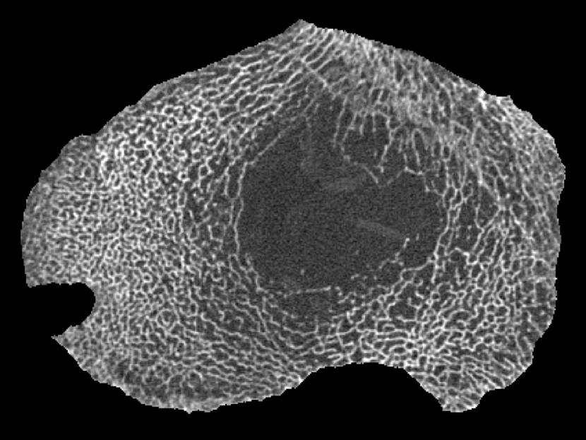
Figure 1: An axial pQCT slice of human proximal tibia acquired 17 mm below the tibial plateau. The cortical shell has been removed from the image. The trabecular BMD of this sample is 107 mg/cm³. The hole visible on the left of the image is the result of a cylindrical biopsy.

Cylindrical bone samples with a diameter of 7 mm were obtained 17 mm distal from the centre of the medial facet of the superior articular surface by drilling with a compressed-air-driven drill with a diamond-tipped trephine at either the right or the left proximal tibia. These bone biopsies were embedded undecalcified in methyl methacrylate, cut in 10-$\mu$m-thick sections on a Jung model K microtome (R. Jung GmbH, Heidelberg, Germany), and stained with aniline blue (modified Masson trichrome). The mounted sections were placed in an flat-bed image scanner and 2540 dpi digital 1 bit images of the sections were obtained as previously described in detail. Thomsen et al. (2005) The resulting pixel size is 10 $\mu$m $\times$ 10 $\mu$m.

The trabecular BMD of each pQCT slice was calculated using a linear relationship derived on the basis of experimental calibration with the European Forearm Phantom, as described by Saparin et al. Saparin et al. (2006) The trabecular BMDs of the slices in this study range from 30 to 150 mg/cm³, with a median of 97  mg/cm³.

III Analytical Method

Most of this section describes the new image analysis method, long range node-strut analysis, which includes the new measure, mean node strength (NdStr). This method was applied to the pQCT sections described in Section II, after removal of the cortical shell. We also computed a standard measures from the same regions of interest of the same pQCT images: trabecular volumetric bone mineral density (BMD), calculated as described by Saparin et al. Saparin et al. (2006)

For further comparison, topological 2-dimensional node-strut analysis Garrahan, Mellish, and Compston (1986) was performed on the histological sections described in Section II, using a custom-made computer program. Thomsen, Ebbesen, and Li. Mosekilde (2000) The trabecular bone profile was iteratively eroded until it was only one pixel thick using a Hilditch skeletonisation procedure, Lam and Suen (1992) and nodes and termini were automatically detected by inspecting the local $3\times 3$ neighbourhood. If the centre pixel of the $3\times 3$ neighbourhood is a skeleton pixel and one and only one of the 8 other pixels is a skeleton pixel the centre pixel is classified as a terminus (Tm) indicating that the strut ends in this pixel. If the centre pixel is a skeleton pixel and three or more of the 8 adjacent pixels are skeleton pixels the centre pixel is classified as a node (Nd) indicating that two or more struts join in this pixel. Compston et al. have argued that the ratio between nodes and termini (Nd/Tm) is an expression of the connectivity of the trabecular network.Compston et al. (1995) Consequently, only the node-to-terminus ratio (Nd/Tm) from this analysis of the histological sections is used in the present study.

III.1 Basic definitions

We start with the algorithm to find strands in each image. A strand is a connected trabecular path, i.e., a chain of one or more struts, with the whole path going in approximately the same direction. In our algorithm, we use eight directions, labelled by the points of the compass: north (N), northeast (NE), east (E), southeast (SE), south (S), southwest (SW), west (W), or northwest (NW). “North” is the anterior direction, which corresponds to “up” in the images shown in this article. A node is a pixel that is joined to strands in at least three of these eight directions, any two of which are at least 90 degrees apart (e.g. N, E, and SW; but not N, NE, and E). The node strength of a pixel is 0 if it is not a node at all, but otherwise depends on the lengths of the strands that meet at the node and the pQCT values of the pixels in these strands.

III.2 CT values of bone

These basic definitions could be implemented in a variety of ways, depending for example on the definitions of “connected” and “same direction”, and on how the pQCT values of the pixels are used. In our algorithm, the first step is to remove marrow from further consideration, by applying a bone threshold filter. The thresholded pQCT values will be referred to in this section as CT values of bone, denoted $b$. Thus if $a$ is the pQCT value of a pixel, then

$$b=\begin{cases}a-a^{\textrm{threshold}}\quad\textrm{if}\quad a>a^{\textrm{threshold}}\\ 0\quad\textrm{otherwise}.\end{cases}$$ (1)

We choose $a^{\textrm{threshold}}=275$, corresponding to a BMD value of 24 mg/cm³. This is the soft tissue threshold used in symbol encoding for complexity measures by Saparin et al. Saparin et al. (2006) The threshold was determined as the pQCT value of the densest non-bone tissue tested, plus the standard deviation of the noise (a calibration protocol for finding the threshold based on a phantom will be developed in the future).

III.3 Strands

In order to explain the central algorithm, we begin by considering a fictitious image consisting of just one row. The CT values of the pixels in the row form a sequence

$$b_{0},b_{1},b_{2},b_{3},\cdots\,.$$

We will define a corresponding sequence of strand strengths,

$$s_{0},s_{1},s_{2},s_{3},\cdots\,,$$

where each $s_{j}$ describes the pattern of densities to the left of pixel $j$ in the row. We begin by setting $s_{0}=0$, and then we recursively define

$$s_{j}=\left(b_{j-1}+Ts_{j-1}\right)\left(\frac{\min\{b_{j},b_{j-1}\}}{b_{j-1}}\right)\,,$$ (2)

where $T$ is a transmission constant between $0$ and $1$. Note that if all of the CT values have a common value $b$ then

$$s_{j} =\left(b+Ts_{j-1}\right)=\left(b+T\left(b+Ts_{j-2}\right)\right)$$

$$=b\left(1+T\right)+T^{2}s_{j-2}=\cdots$$

$$=b\left(1+T+\cdots+T^{j}\right),$$

since $s_{0}=0$. As $j$ increases, $s_{j}$ approaches an upper bound of $\dfrac{b}{1-T}$. Thus, for the simple case of a uniformly dense row, we have defined the strand strength to be $\dfrac{1}{1-T}$ times the CT values of bone. This constant $\dfrac{1}{1-T}$ can be interpreted as a characteristic length of the method, which we can vary depending on the length of strand that we believe to be most important to the strength of the bone. For the present study, we have chosen $T=0.95$, corresponding to a characteristic length of $20$ pixels, i.e. 4 mm. For the general case of a variable CT values row, the presence of the transmission constant $T$ in the recursive formula ensures that the CT value of pixels closest to the $j^{\textrm{th}}$ pixel have the greatest effect on $s_{j}$. Finally, the factor $\dfrac{\min\{b_{j},b_{j-1}\}}{b_{j-1}}$ ensures that $s_{j}$ depends strongly on $b_{j}$, so that any weak link in a chain of high-density pixels lowers the strand strength dramatically.

The difficulty in generalising this definition to a 2-dimensional image is of course that there are infinitely many directions but only four that are parallel with the pixel grid. We have resolved this in a practical but ad hoc fashion. As already stated, we consider eight directions. Consider first the definition of strand strength in the leftwards (W) direction. ¿From pixel $(i,j)$ (at row $i$ and column $j$) we consider that there are five length-3 paths leading approximately leftwards:

$$(\text{i})\hfill (i+1,j-2) \leftarrow(i+1,j-1)\leftarrow(i,j),$$

$$(\text{ii})\hfill (i+1,j-2) \leftarrow(i,j-1)\leftarrow(i,j),$$

$$(\text{iii})\hfill (i,j-2) \leftarrow(i,j-1)\leftarrow(i,j),$$

$$(\text{iv})\hfill (i-1,j-2) \leftarrow(i,j-1)\leftarrow(i,j),$$

$$(\text{v})\hfill (i-1,j-2) \leftarrow(i-1,j-1)\leftarrow(i,j),$$

as illustrated in Fig. 2.

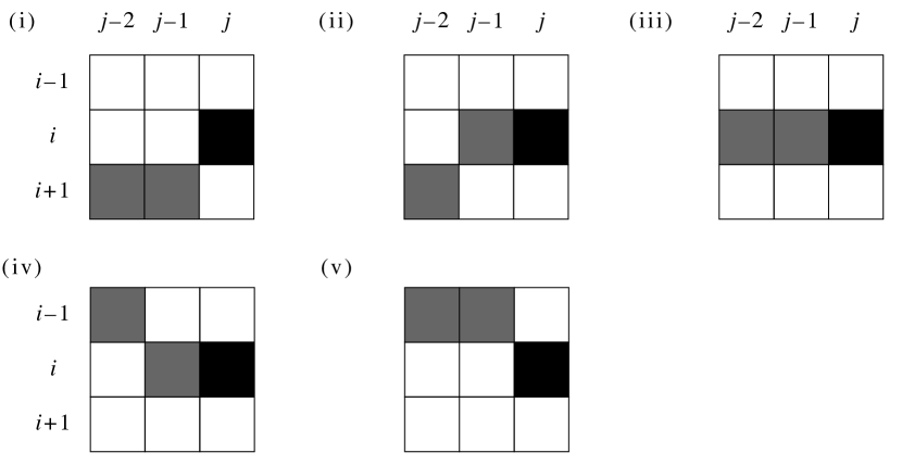
Figure 2: The five possible length-3 paths in a leftwards (“west”) direction from pixel $(i,j)$. The start pixel $(i,j)$ is marked in black.

III.4 Strand strength

For each of these paths, we define $b_{j},b_{j-1}$ and $b_{j-2}$ as the CT values of the pixels in the path in columns $j,j-1$, and $j-2$. We then apply the recursive formula

$$s_{j} = \left(b_{j-1}+T\left(b_{j-2}+Ts_{j-2}\right)\left(\frac{\min\{b_{j-1},b_{j-2}\}}{b_{j-2}}\right)\right)$$ (3)

$$\times\left(\frac{\min\{b_{j},b_{j-1}\}}{b_{j-1}}\right),$$

which is the formula in Eq. (2), applied twice. (We must now set $s_{1}=s_{0}=0$.) We now have five $s_{j}$ values, one for each of the five paths, i.e., $s_{j}^{(i)},\ s_{j}^{(ii)},\ldots,s_{j}^{(v)}$. We multiply all but the third (Fig. 2(iii)) of these five values by a bending coefficient $\gamma$ between $0$ and $1$, to penalise strands that bend away from the horizontal direction. Then the maximum of these five numbers is our leftwards (W) strand strength $S^{W}_{ij}=\max\{\gamma s_{j}^{(i)},\ \gamma s_{j}^{(ii)},\ s_{j}^{(iii)},\ \gamma s_{j}^{(iv)},\ \gamma s_{j}^{(v)}\}$.

Strand strengths in the other seven directions $S^{NW}_{ij},\ S^{N}_{ij},\ S^{NE}_{ij},\ldots,S^{SW}_{ij}$ are determined in a similar manner. For diagonal directions, the geometry of the five length-3 paths used in the computation is slightly different, so a different bending coefficient $\gamma$ is used. We chose $\gamma=0.6$ for the horizontal and vertical directions and $\gamma=0.8$ for the diagonal directions. These constants were chosen so as to give mean strand strengths that are approximately invariant to image rotations by an arbitrary angle, which were verified by numerical experiments on tibial images.

III.5 Node strength

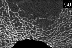
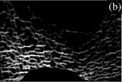
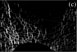
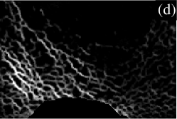
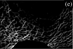
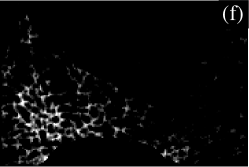
Figure 3: Node strength algorithm illustrated on a region of trabecular bone taken from the full section shown in Fig. 1. (a) original image; (b) horizontal strands; (c) vertical strands; (d) diagonal strands (“northwest - southeast”); (e) diagonal strands (“northeast - southwest”); (f) node strength.

Finally, we calculate the node strength $\sigma_{ij}$ at each pixel. There are $k=16$ possible ways of choosing 3 out of the 8 directions in such a way that each pair of chosen directions makes an angle of at least 90 degrees. For example, E, N, and SW comprise an allowable choice, but E, N, and NE do not. At each pixel, for each allowable choice of three directions, we calculate the minimum of the three strand strengths in these directions, e.g., $\hat{S}_{ij}^{k}=\min\{S^{E}_{ij},\ S^{N}_{ij},\ S^{SW}_{ij}\}$. The node strength $\sigma_{ij}$ is the maximum of the 16 minima $\hat{S}_{ij}^{k}$ subtracted by a minimum strength constant $S_{0}$,

$$\sigma_{ij}=\max_{k=1\ldots 16}\big{\{}\hat{S}_{ij}^{k}\big{\}}-S_{0}.$$ (4)

Pixels with a positive node strength are called nodes. The mean node strength over the region of interest (ROI) is called the node strength of the region,

$$\text{NdStr}=\frac{1}{\text{ROI}}\sum_{ij\in\text{ROI}}\sigma_{ij}.$$ (5)

The purpose of subtracting the minimum strength constant $S_{0}$ is to allow us to ignore short “strands”, which are often just transverse sections of trabeculae with an apparent width of more than one pixel. The trabeculae in our images have an apparent width of approximately two pixels, or 0.4 mm, which is higher than the true average trabecular width, due to the 1 mm thickness of the CT image and the 0.2 mm pixel size. Thus, we wish to ignore strands of bone that are only two pixels long. The strength of such a strand depends on the pQCT values of the two pixels. Following Eq. (2), the strength $s$ of such a strand with CT value $b_{0}=b_{1}=b$ is $s=b$. Based on examination of the resulting node strength images (such as Fig. 3 (f)), we find ad hoc a minimum strength constant of 225 (corresponding to a CT value of 500, Eq. (1), corresponding to a BMD value of 331 mg/cm³, which is higher than the mean CT value for trabecular bone). So strands of lower strength than this will be ignored by the algorithm.

We note that our complete algorithm involves two thresholding steps: one at the beginning, when pQCT values are converted to CT values of bone; and one at the end, when the minimum strength constant is subtracted. These are not equivalent to one thresholding step with a higher threshold. The purpose of the first threshold filtration is to ignore marrow. The purpose of the second threshold filtration is to ignore short strands, and it can be seen as an alternative to skeletonisation.

Numerical experiments have shown that relative (cross-subject) values of NdStr are stable with respect to the choice of the bone threshold value ($a^{\textrm{threshold}}$) and minimum strength constant. Specifically, if either of these constants is varied by $\pm 10\%$ from the values used in this article, and NdStr is recomputed for all subjects, the resulting NdStr values are very strongly linearly correlated with the original NdStr values (Pearson correlation coefficient $r>0.995$ in all cases). The absolute values of NdStr depend on the choice of these constants: increasing the bone threshold by $10\%$ leads to a $40\%$ mean decrease in NdStr (percent decrease averaged over all subjects), while increasing the minimum strength constant by $10\%$ leads to an average decrease in NdStr of $11\%$. Nevertheless, and as already mentioned, the relative (cross-subject) variation of NdStr remains constant.

A key property of NdStr is that it depends on both the geometry of the trabecular network and the CT values of the trabeculae. NdStr depends linearly on thresholded CT values, if the CT values of all pixels are varied by the same factor. It follows that images with the same geometry but different BMD will have different NdStr values. On the other hand, two images with the same BMD but different geometry can have different NdStr values. This is apparent from the description of the method, and confirmed by Figs. 4 and 5, as discussed below, and also by the results discussed in Section IV.

III.6 Illustration

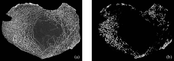
Figure 4: Trabecular micro-architecture of a section with BMD 107 mg/cm³. (a) original image; (b) the node strength of each pixel. The mean node strength is 71.2.

To illustrate the analytical method, we now present the results in visual form for an enlarged region near the bottom (posterior) of the slice in Fig. 1. The enlarged region of the original image is shown in Fig. 3(a). Parts (b) to (e) of Fig. 3 show directional strand strengths, and part (f) shows the final node strength plot. Each directional strand strength plot shows the sum of two strand strengths at every pixel, in opposite directions: east/west; north/south; northwest/southeast; and northeast/southwest. In each of the directional strand strength plots, the strands in the given direction are shown with the highest intensity, but most of the trabeculae are still visible, even if faintly. In contrast, in the node strength plot (part (f)), most of the trabeculae are invisible. This is because of the subtraction of the minimum strength constant. In this example, there are almost no nodes in the right half of the image. This correctly describes the micro-architecture of the original image in that region, which contains many trabeculae but few that cross each other to make a lattice-like micro-architecture. The left half of the image contains many nodes. Notice that, in the node strength plot, the nodes seem to be thicker than in the original image. This is because the trabeculae in the original image are actually slightly thicker than they appear, the outer pixels being dimmer (i.e. lower CT values) and thus not easily registered by the eye. Since the outer pixels near the apparent nodes in the original image are almost as well-connected as pixels in the centres of the nodes, they have large node strengths, and are very visible in the node strength plot.

The two specimens depicted in Figs. 4 and 5 have comparable bone mineral densities, but their trabecular micro-architecture are visibly different. In Fig. 4, the specimen has a trabecular BMD of 107 mg/cm³, which is near the median value (97 mg/cm³) of the specimens in this study. On the left is the original image, and on the right is the node strength plot. Notice that there are a lot of nodes in most of the outer areas, with the notable exception of a region near the bottom left. The mean node strength is 71.2.

The specimen in Fig. 5 has a trabecular BMD of 94  mg/cm³, which is only 12% lower than that of the specimen shown in Fig. 4, but it has substantially fewer nodes. The mean node strength is only 42.2, which is 40% lower than that for the specimen shown in Fig. 4. This reflects the lack of a strong lattice-like micro-architecture in the original image.

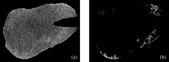
Figure 5: Trabecular micro-architecture of a section with BMD is 94 mg/cm³. (a) original image; (b) the node strength of each pixel. The mean node strength is 42.2.

IV Results

The long range node strength of each pixel of each image was computed as described in the previous section, and a mean node strength, NdStr, was calculated for each image. We also computed the bone mineral density (BMD) from the pQCT slices, as explained in Section III. A scatter plot showing NdStr versus BMD for all 26 specimens is shown in Fig. 6. There is a strong positive correlation, which we quantified in three ways. Firstly, Pearson’s correlation coefficient is $r=0.87$, indicating a very strong linear correlation. Secondly, since the scatter plot clearly suggests a nonlinear relationship, we fitted an exponential curve to the data and then found Pearson’s correlation coefficient to be $r=0.97$. Thirdly, the Spearman rank correlation is $\rho=0.98$, indicating a very strong correlation. The Spearman rank correlation coefficient is a robust nonparametric correlation measure that is appropriate when little is known about the distributions and nature of the correlation between the variables. Press et al. (1992)

We also compared NdStr with the node-terminus ratio, Nd/Tm, in the topological node-strut analysis introduced by Garrahan et al. Garrahan, Mellish, and Compston (1986) The two measures are similar in philosophy, because they both quantify the nodes in the trabecular network. However, the definition of Nd/Tm is highly localised: after the skeletonisation process has eroded the trabecular network to a thickness of one pixel, each pixel is classified as node, strut, or terminus depending on its $3\times 3$ grid of nearest neighbours (including the original pixel). For the present study, the images used to compute Nd/Tm have a pixel size of $10\,\mu$m, so the classification is made on the basis of a 30 $\mu$m $\times$ 30 $\mu$m region. In contrast, node strength is semi-global, taking into account longer strands to a degree controlled by the transmission strength constant. In the present study, with this constant set to $0.95$, the method has a characteristic length of 4 mm, in the sense described in Section III.

The node-terminus ratio, Nd/Tm, was calculated using histomorphometry performed on bone biopsies as described in Section III. Recall that these biopsies were from the same regions of the same donors as the pQCT slices from which NdStr has been computed. Pearson’s correlation coefficient for the relationship between NdStr and Nd/Tm is $r=0.62$, and the Spearman rank correlation coefficient is $\rho=0.65$. We also measured the correlation between Nd/Tm and trabecular BMD: Pearson’s correlation coefficient is $r=0.64$, and the Spearman rank correlation coefficient is $\rho=0.61$. Using either measure of correlation, mean node strength is more strongly correlated with trabecular BMD than the node-terminus ratio is correlated with either of these variables.

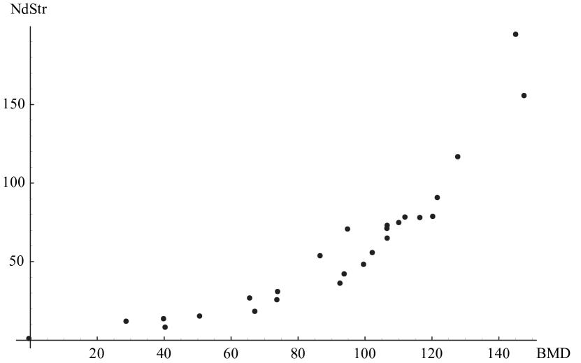
Figure 6: Scatter plot of mean node strength vs. trabecular bone mineral density (mg/cm³).

V Discussion

We have introduced a new morphometric measure for characterising the micro-architecture of trabecular bone, long range node strength, which measures the degree to which a pixel in a 2-dimensional bone image has long-range connectivity in three or more directions, each at least 90 degrees from the others. In addition, we have calculated the mean node strength, NdStr, for each of the 26 bone samples considered in the study. We have found that NdStr has a strong positive correlation with trabecular BMD ($r=0.97$, after exponential transformation). Furthermore, we have ascertained a strong correlation ($r=0.62$) between NdStr and the established histomorphometric measure, node-terminus ratio (Nd/Tm). Moreover, qualitative comparison of images with similar trabecular BMD but different mean NdStr (see Figs. 4 and 5) suggest that NdStr successfully quantifies how “lattice-like” the micro-architecture is.

Further studies, including either clinical data or measured bone strength, are needed in order to determine the utility of this measure relative to other existing morphometric measures. Such studies could also determine the most useful choice of the parameters that appear in the algorithm: the transmission constant, minimum strength constant, and bending coefficients. For example, these constants could be chosen to maximise correlations with bone strength. In the future, the sensitivity of the method on these parameters and on different CT settings (e.g., CT pixel size, slice thickness, mean CT value of bone) should be systematically investigated. Moreover, a future study on synthetic data could be used to verify that NdStr measures structure and not just bone volume or mass, and specifically that it finds nodes. Also different skeletal sites should be analysed with our approach in order to test its potential to describe structural differences.

We would like to note that our algorithm for computing node strength is dependent on pixel size, and is thus unsuitable for absolute comparisons between studies. However, this limitation is not unique to the node strength measure. For example, Guggenbuhl et al. have showed using CT images with different thickness (1 mm, 3 mm, 5 mm, and 8 mm) that the outcome of texture analysis depends substantially on the slice thicknessGuggenbuhl et al. (2008). In the present study we have used pQCT equipment with an in-plane pixel size of 200 $\mu$m $\times$ 200 $\mu$m and a slice thickness of 1 mm. We have not conducted a formal investigation into the influence of slice thickness on the long range node strength, but it is fair to assume that the long range node strength is similarly affected by the slice thickness. If further studies were to confirm the practical value of the measure, an implementation could be developed to produce node strengths that are broadly comparable between images with different pixel size. However, the technological development of high-resolution pQCT equipment is progressing very quickly, and already high-resolution pQCT scanners exist that can image a tibia at an isotropic pixel size of approximately 100 $\mu$m, which is comparable to the trabecular thickness in the human proximal tibiaDing and Hvid (2000), thus making the slice thickness less of an issue.

Some previous studies have investigated the trabecular bone micro-architecture using texture analysis applied on X-ray images of boneGeraets et al. (1990); Chappard et al. (2005, 2006); Huber et al. (2009); Korstjens et al. (1996). However, these techniques are not comparable to the method presented in the present study as they are based on projections of a 3-dimensional trabecular network on a 2-dimensional plane, whereas our method is applied to 2-dimensional sections obtained through the 3-dimensional trabecular network. Nevertheless, Ranjanomennahary et al. very recently showed some significant correlation did exist between radiograph based texture analysis and $\mu$CT based unbiased 3-dimensional measures of trabecular micro-architectureRanjanomennahary et al. (2011). Apostol et al. compared 3-dimensional measures of micro-architecture based on 3-dimensional synchrotron radiation CT with more than 350 texture parameters obtained from simulated radiographs that were created from the synchrotron radiation CT data setsApostol et al. (2006). They found using multiple regression analysis that a combination of a subset of texture analysis parameters correlated to the 3-dimensional measures of micro-architecture. However, they had to use at least three texture analysis parameters in the correlation with each of the 3-dimensional measures of micro-architecture. Cortet et al. investigated CT images of the distal radius using texture analysisCortet et al. (2000, 1999). The CT image used by Cortet et al. used similar pixel size to those used in the present study. They analysed the CT images using the traditional node-strut analysis and texture analysis including the grey level run length methodChu, Sehgal, and Greenleaf (1990); Galloway (1975). As illustrated in the present work there is a moderate correlation ($r=0.64$) between the node-strut analysis and the NdStr measure, which we believe illustrates that the NdStr measure captures somewhat different information from that obtained with the node-strut analysis. Grey level run length is based on runs that have exactly the same grey level, and is therefore very sensitive to the choice of discretisation of the grey levels. In contrast, the NdStr measure treats the grey level as a continuous parameter, and thus it is able to detect runs with variable grey levels, and is consequently less sensitive to discretisation choices.

Another advantage of the method is that the proposed method utilises all of the CT value information in the pQCT images, as no binarization of the images is performed.

In the present study we have not applied the developed method to the histological sections directly. The reason for this is that the histological sections only cover a limited area of interest and thereby a limited trabecular length, which renders the NdStr less meaningful. However, this is a limitation of the histological examination procedure where it is only feasible to investigate a smaller sample (biopsy) of a larger structure (the proximal tibia) and not a limitation of the proposed method. In addition, the histological images are segmented into bone and marrow by their nature and it is thus not possible to assign an intensity value to pixels, analogous to a CT value, which is needed by the algorithm in its present form. However, it is possible to apply the concept of long range node-strut analysis to such binary images but this is outside the scope of the present investigation.

In the present study the long range node-strut analysis was applied to pQCT images of the proximal tibia. However, we would like to stress that the method is not limited to this skeletal site and thus can be applied to 2-dimensional CT images obtained from any skeletal site like e.g. the vertebral body or the calcaneous.

Finally, we note that the general method of long range node-strut analysis provides more than just the mean node strength. In the present study, we have focused on mean node strength for simplicity, but the intermediate measures of directional strand strength, used in the computation of node strength, may be useful in themselves as a measure of directional strength. In the present study the long range node-strut analysis has been applied to 2-dimensional pQCT images obtained in the horizontal plane. However, the trabecular micro-architecture of the proximal tibia is mostly isotropic in the horizontal plane, whereas the micro-architecture in vertical direction is highly anisotropic compared with the horizontal planeDing et al. (2002). As $\mu$CT scanners become more and more prevalent and as the pixel size and imaging capacity of pQCT scanners steadily improve it will be an important future task to generalise the long range node-strut analysis into three dimensions and to apply the technique to 3-dimensional data sets obtained from such equipment. In particular, the directional strand strength could be used to investigate anisotropic differences of the trabecular micro-architecture of such 3-dimensional data sets.

References

- Goldstein, Goulet, and McCubbrey (1993) S. A. Goldstein, R. Goulet, and D. McCubbrey, “Measurement and Significance of Three-Dimensional Architecture to the Mechanical Integrity of Trabecular Bone,” Calcified Tissue 53, S127–S133 (1993).
- Li. Mosekilde, Viidik, and Le. Mosekilde (1985) Li. Mosekilde, A. Viidik, and Le. Mosekilde, “Correlation Between the Compressive Strength of Iliac and Vertebral Trabecular Bone in Normal Individuals,” Bone 6, 291–295 (1985).
- Delling and Amling (1995) G. Delling and M. Amling, “Biomechanical stability of the skeleton – it is not only bone mass, but also bone structure that counts,” Nephrology Dialysis Transplantation 10, 601–606 (1995).
- Rho, Kuhn-Spearing, and Zioupos (1998) J.-Y. Rho, L. Kuhn-Spearing, and P. Zioupos, “Mechanical properties and the hierarchical structure of bone,” Medical Engineering & Physics 20, 92–102 (1998).
- Hildebrand et al. (1999) T. Hildebrand, A. Laib, R. Müller, J. Dequeker, and P. Rüegsegger, “Direct Three-Dimensional Morphometric Analysis of Human Cancellous Bone: Microstructural Data from Spine, Femur, Iliac Crest, and Calcaneus,” Journal of Bone and Mineral Research 14, 1167–1174 (1999).
- Rajapakse et al. (2004) C. S. Rajapakse, J. S. Thomsen, J. S. Espinoza Ortiz, S. J. Wimalawansa, E. N. Ebbesen, Li. Mosekilde, and G. H. Gunaratne, “An expression relating breaking stress and density of trabecular bone,” Journal of Biomechanics 37 (2004), 10.1016/j.jbiomech.2003.12.001.
- Kinney et al. (2005) J. H. Kinney, J. S. Stölken, T. S. Smith, J. T. Ryaby, and N. E. Lane, “An orientation distribution function for trabecular bone,” Bone 36, 193–201 (2005).
- Eastell et al. (1990) R. Eastell, Li. Mosekilde, S. F. Hodgson, and B. L. Riggs, “Proportion of human vertebral body bone that is cancellous,” Journal of Bone and Mineral Research 5, 1237–1241 (1990).
- Ritzel et al. (1997) H. Ritzel, M. Amling, M. Pösel, M. Hahn, and G. Delling, “The Thickness of Human Vertebral Cortical Bone and Its Changes in Aging and Osteoporosis: A Histomorphometric Analysis of the Complete Spinal Column from Thirty-Seven Autopsy Specimens,” Journal of Bone and Mineral Research 12, 89–95 (1997).
- McDonnell, McHugh, and O’Mahoney (2007) P. McDonnell, P. E. McHugh, and D. O’Mahoney, “Vertebral osteoporosis and trabecular bone quality,” Annals of Biomedical Engineering 35, 170–189 (2007).
- Carter and Hayes (1977) D. R. Carter and W. C. Hayes, “The Compressive Behaviour of Bone as a Two-Phase Porous Structure,” The Journal of Bone and Joint Surgery 59A, 954–962 (1977).
- Ebbesen et al. (1999) E. N. Ebbesen, J. S. Thomsen, H. Beck-Nielsen, H. J. Nepper-Rasmussen, and Li. Mosekilde, “Lumbar Vertebral Body Compressive Strength Evaluated by Dual-Energy X-ray Absorptiometry, Quantitative Computed Tomography, and Ashing,” Bone 25, 713–724 (1999).
- Jiang et al. (1998) Y. Jiang, J. Zhao, P. Augat, X. Ouyang, Y. Lu, S. Majumdar, and H. K. Genant, “Trabecular bone mineral and calculated structure of human bone specimens scanned by peripheral quantitative computed tomography: Relation to biomechanical properties,” Journal of Bone and Mineral Research 13, 1783–1790 (1998).
- Majumdar et al. (1998) S. Majumdar, M. Kothari, P. Augat, D. C. Newitt, T. M. Link, J. C. Lin, T. Lang, Y. Lu, and H. K. Genant, “High-resolution magnetic resonance imaging: Three-dimensional trabecular bone architecture and biomechanical properties,” Bone 22, 445–454 (1998).
- Odgaard et al. (1997) A. Odgaard, J. Kabel, B. van Rietbergen, M. Dalstra, and R. Huiskes, “Fabric and elastic principal directions of cancellous bone are closely related,” Journal of Biomechanics 30, 487–495 (1997).
- Ulrich et al. (1999) D. Ulrich, B. van Rietbergen, A. Laib, and P. Rüegsegger, “The ability of three-dimensional structural indices to reflect mechanical aspects of trabecular bone,” Bone 25, 55–60 (1999).
- Baum et al. (2010) T. Baum, J. Carballido-Gamio, M. B. Huber, D. Müller, R. Monetti, C. Räth, F. Eckstein, E. M. Lochmüller, S. Majumdar, E. J. Rummeny, T. M. Link, and J. S. Bauer, “Automated 3d trabecular bone structure analysis of the proximal femur—prediction of biomechanical strength by ct and dxa,” Osteoporosis International 21, 1553–1564 (2010).
- Thomsen, Ebbesen, and Li. Mosekilde (1998) J. S. Thomsen, E. N. Ebbesen, and Li. Mosekilde, “Relationships Between Static Histomorphometry and Bone Strength Measurements in Human Iliac Crest Bone Biopsies,” Bone 22, 153–163 (1998).
- Thomsen, Ebbesen, and Li. Mosekilde (2002) J. S. Thomsen, E. N. Ebbesen, and Li. Mosekilde, “Predicting Human Vertebral Bone Strength by Vertebral Static Histomorphometry,” Bone 30, 502–508 (2002).
- Saparin et al. (1998) P. I. Saparin, W. Gowin, J. Kurths, and D. Felsenberg, “Quantification of cancellous bone structure using symbolic dynamics and measures of complexity,” Physical Review E 58, 6449 (1998).
- Dougherty (2001) G. Dougherty, “A comparison of the texture of computed tomography and projection radiography images of vertebral trabecular bone using fractal signature and lacunarity,” Med Eng Phys 23, 313–321 (2001).
- Prouteau et al. (2004) S. Prouteau, G. Ducher, P. Nanyan, G. Lemineur, L. Benhamou, and D. Courteix, “Fractal analysis of bone texture: a screening tool for stress fracture risk?” European Journal of Clinical Investigation 34, 137–142 (2004).
- Saparin et al. (2005) P. I. Saparin, J. S. Thomsen, S. Prohaska, A. Zaikin, J. Kurths, H.-C. Hege, and W. Gowin, “Quantification of spatial structure of human proximal tibial bone biopsies using 3D measures of complexity,” Acta Astronautica 56, 820–830 (2005).
- Saparin et al. (2006) P. I. Saparin, J. S. Thomsen, J. Kurths, G. Beller, and W. Gowin, “Segmentation of bone ct images and assessment of bone structure using measures of complexity,” Med. Phys. 33, 3857–3873 (2006).
- Marwan, Kurths, and Saparin (2007) N. Marwan, J. Kurths, and P. Saparin, “Generalised Recurrence Plot Analysis for Spatial Data,” Physics Letters A 360, 545–551 (2007).
- Marwan, Saparin, and Kurths (2007) N. Marwan, P. Saparin, and J. Kurths, “Measures of complexity for 3D image analysis of trabecular bone,” The European Physical Journal – Special Topics 143, 109–116 (2007).
- Marwan et al. (2009) N. Marwan, J. Kurths, J. S. Thomsen, D. Felsenberg, and P. Saparin, “Three dimensional quantification of structures in trabecular bone using measures of complexity,” Physical Review E 79, 021903 (2009).
- van Rietbergen et al. (1998) B. van Rietbergen, S. Majumdar, W. Pistoia, D. C. Newitt, M. Kothari, A. Laib, and P. Rüegsegger, “Assessment of cancellous bone mechanical properties from micro-FE models based on micro-CT, pQCT and MR images,” Technology and Health Care 6, 413–420 (1998).
- Guo and Kim (2002) X. E. Guo and C. H. Kim, “Mechanical Consequence of Trabecular Bone Loss and Its Treatment: A Three-dimensional Model Simulation,” Bone 30, 404–411 (2002).
- Pothuaud et al. (2002) L. Pothuaud, B. Van Rietbergen, L. Mosekilde, O. Beuf, P. Levitz, C. L. Benhamou, and S. Majumdar, “Combination of topological parameters and bone volume fraction better predicts the mechanical properties of trabecular bone,” Journal of Biomechanics 35, 1091–1099 (2002).
- Wolfram et al. (2009) U. Wolfram, L. O. Schwen, U. Simon, and M. Rumpf, “Statistical osteoporosis models using composite finite elements: A parameter study,” Journal of Biomechanics 42, 2205–2209 (2009).
- Garrahan, Mellish, and Compston (1986) N. J. Garrahan, R. W. E. Mellish, and J. E. A. Compston, “A new method for the two-dimensional analysis of bone structure in human iliac crest biopsies,” Journal of Microscopy 142, 341–349 (1986).
- Saparin, Gowin, and Felsenberg (2002) P. Saparin, W. Gowin, and D. Felsenberg, “Comparison of bone loss with the changes of bone architecture at six different skeletal sites using measures of complexity,” Journal of Gravitational Physiology 9, 177–178 (2002).
- Thomsen et al. (2005) J. S. Thomsen, A. Laib, B. Koller, S. Prohaska, Li. Mosekilde, and W. Gowin, “Stereological measures of trabecular bone structure: comparison of 3D micro computed tomography with 2D histological sections in human proximal tibial bone biopsies,” Journal of Microscopy 218, 171–179 (2005).
- Thomsen, Ebbesen, and Li. Mosekilde (2000) J. S. Thomsen, E. N. Ebbesen, and Li. Mosekilde, “A New Method of Comprehensive Static Histomorphometry Applied on Human Lumbar Vertebral Cancellous Bone,” Bone 27, 129–138 (2000).
- Lam and Suen (1992) L. Lam and C. Y. Suen, “Thinning methodologies – a comprehensive survey,” IEEE Transaction on Pattern Analysis and Machine Intelligence 14, 869–885 (1992).
- Compston et al. (1995) J. E. Compston, K. Yamaguchi, P. I. Croucher, N. J. Garrahan, P. C. Lindsay, and R. W. Shaw, “The effects of gonadotrophin-releasing hormone agonists on iliac crest cancellous bone structure in women with endometriosis,” Bone 16, 261–267 (1995).
- Press et al. (1992) W. H. Press, S. A. Teukolsky, W. T. Vetterling, and B. P. Flannery, Numerical Recipes in C — the Art of Scientific Computing, 2nd ed. (Cambridge University Press, Cambridge, 1992).
- Ding et al. (2002) M. Ding, A. Odgaard, F. Linde, and I. Hvid, “Age-related variations in the microstructure of human tibial cancellous bone,” Journal of Orthopaedic Research 20, 615–621 (2002).
- Guggenbuhl et al. (2008) P. Guggenbuhl, D. Chappard, M. Garreau, J.-Y. Bansard, G. Chales, and Y. Rolland, “Reproducibility of ct-based bone texture parameters of cancellous calf bone samples: Influence of slice thickness,” European Journal of Radiology 67, 514–520 (2008).
- Ding and Hvid (2000) M. Ding and I. Hvid, “Quantification of age-related changes in the structure model type and trabecular thickness of human tibial cancellous bone,” Bone 26, 291–295 (2000).
- Geraets et al. (1990) W. G. M. Geraets, P. F. van der Stelt, C. J. Netelenbos, and P. J. M. Elders, “A new method for automatic recognition of the radiographic trabecular pattern,” Journal of Bone and Mineral Research 5, 227–233 (1990).
- Chappard et al. (2005) D. Chappard, P. Guggenbuhl, E. Legrand, M. F. Baslé, and M. Audran, “Texture analysis of x-ray radiographs is correlated with bone histomorphometry,” Journal of Bone and Mineral Metabolism 23, 24–29 (2005).
- Chappard et al. (2006) D. Chappard, F. Pascaretti-Grizon, Y. Gallois, P. Mercier, M. F. Baslé, and M. Audran, “Medullar fat influences texture analysis of trabecular microarchitecture on x-ray radiographs,” European Journal of Radiology 58, 404–410 (2006).
- Huber et al. (2009) M. B. Huber, J. Carballido-Gamio, K. Fritscher, R. Schubert, M. Haenni, C. Hengg, S. Majumdar, and T. M. Link, “Development and testing of texture discriminators for the analysis of trabecular bone in proximal femur radiographs,” Medical Physics 36, 5089–5098 (2009).
- Korstjens et al. (1996) C. M. Korstjens, Li. Mosekilde, R. J. Spruijt, W. G. M. Geraets, and P. F. van der Stelt, “Relations between radiographic trabecular pattern and biomechanical characteristics of human vertebrae,” Acta Radiologica 37, 618–624 (1996).
- Ranjanomennahary et al. (2011) P. Ranjanomennahary, S. S. Ghalila, D. Malouche, A. Marchadier, M. Rachidi, C. Benhamou, and C. Chappard, “Comparison of radiograph-based texture analysis and bone mineral density with three-dimensional microarchitecture of trabecular bone,” Medical Physics 38, 420–428 (2011).
- Apostol et al. (2006) L. Apostol, V. Boudousq, O. Basset, C. Odet, S. Yot, J. Tabary, J.-M. Dinten, E. Boiler, P.-O. Kotzki, and F. Peyrin, “Relevance of 2d radiographic texture analysis for the assessment of 3d bone micro-architecture,” Medical Physics 33, 3546–3556 (2006).
- Cortet et al. (2000) B. Cortet, N. Boutry, P. Dubois, P. Bourel, A. Cotten, and X. Marchandise, “In vivo comparison between computed tomography and magnetic resonance image analysis of the distal radius in the assessment of osteoporosis,” Journal of Clinical Densitometry 3, 15–26 (2000).
- Cortet et al. (1999) B. Cortet, P. Dubois, N. Boutry, P. Bourel, A. Cotten, and X. Marchandise, “Image analysis of the distal radius trabecular network using computed tomography,” Osteoporosis International 9, 410–419 (1999).
- Chu, Sehgal, and Greenleaf (1990) A. Chu, C. M. Sehgal, and J. F. Greenleaf, “Use of gray value distribution of run lengths for texture analysis,” Pattern Recognition Letters 11, 415–420 (1990).
- Galloway (1975) M. M. Galloway, “Texture analysis using gray level run lengths,” Computer Graphics and Image Processing 4, 172–179 (1975).