Temperature dependence of the magnetic hyperfine field at an s-p impurity diluted in $R$Ni₂

Abstract

We study the formation of local magnetic moments and magnetic hyperfine fields at an s-p impurity diluted in intermetallic Laves phases compounds $R$Ni₂ ($R$ = Nd, Sm, Gd, Tb, Dy) at finite temperatures. We start with a clean host and later the impurity is introduced. The host has two-coupled ($R$ and Ni) sublattice Hubbard Hamiltonians but the Ni sublattice can be disregarded because its d band, being full, is magnetically ineffective. Also, the effect of the 4f electrons of $R$ is represented by a polarization of the d band that would be produced by the 4f magnetic field.This leaves us with a lattice of effective rare earth R-ions with only d electrons. For the dd electronic interaction we use the Hubbard-Stratonovich identity in a functional integral approach in the static saddle point approximation.

I introduction

The Laves phases intermetallic compounds $R$Ni₂ ($R$ = rare earth elements ) crystallize in a cubic structure Buschow77 and exhibit an interesting variety of behaviors related to the changes in their magnetic, electronic, and lattice structures. They exhibit magnetization associated both with the localized spins ($4f$) and with the itinerant electrons of the rare earth. Although the extensive studies made, the theoretical description of how some of their properties varies with temperature, due to the electronic correlations, still remains open. The Ni sublattice however can be disregarded because its d band, being full, is magnetically ineffective. Also the effect of the $R$ 4f electrons is represented by a polarized d band produced by the 4f electrons magnetic field. This approximation generates an effective rare earth R lattice but whose interactions differ from the usual $R$ pure metal because now the equivalent lattice constant is different (see the end of section $\bf{III}$ for a numerical indication of the difference between the two cases).

II Method

II.1 The effective host

We start with a clean effective host described by the Hamiltonian of itinerant d-electrons:

$$\mathcal{H}=H_{d}^{0}+H_{d}^{1}.$$ (1)

The first term of Eq.(1) is

$$H_{d}^{0}=\sum_{l\sigma}\varepsilon_{0\sigma}d_{l\sigma}^{\dagger}d_{l\sigma}+\sum_{ll^{\prime}\sigma}T_{ll^{\prime}}d_{l\sigma}^{\dagger}d_{l^{\prime}\sigma},$$ (2)

where $\varepsilon_{0\sigma}$ is the energy of the center of the d band, now depending on the spin polarization; $d_{j\sigma}^{\dagger}$ ($d_{j\sigma}$) is creation (annihilation) operators, and $T_{ll^{\prime}}$ is the hopping integrals between atoms from the $R$ effective lattice.

$H_{d}^{1}$ represents the Coulomb interaction

$$H_{d}^{1}=U\sum_{l}n_{l\uparrow}n_{l\downarrow},$$ (3)

$n_{l\sigma}$ being the number operator.

The partition function $\mathcal{Z}$ for the system described by Hamiltonian (1) can be written as

$$\mathcal{Z} = \int\prod_{l}\,\mathrm{d}\nu_{l}\,\mathrm{d}\xi_{l}\int\prod_{j}\,\mathrm{d}\nu_{j}\,\mathrm{d}\xi_{j}\,e^{{}^{-\beta\left[-\frac{U}{4}\sum_{l}\left(\nu_{l}^{2}+\xi_{l}^{2}\right)\right]}}$$ (4)

$$\times\mathrm{tr}\,e^{-\beta\left(H_{d}^{0}-\frac{U}{2}\sum_{l\sigma}\left(i\nu_{l}+\sigma\xi_{l}\right)n_{l\sigma}\right)}\cdot$$

where $\beta=1/k_{\mathrm{B}}T$, $k_{\mathrm{B}}$ is the Boltzman constant and $T$ the temperature. The Hubbard-Stratonovich identityHS was used in order to linearize the Coulomb interaction generating two floating fields, an electric, $\nu_{l}$, and a magnetic, $\xi_{l}$. The static approximation has also been performed.

Now, because of the floating fields, the system, although pure, becomes disorderedIF1 ; IF2 . In Eq.(4) we see that the floating fields create site dependent $\varepsilon_{l_{0}\sigma}$’s :

$$\varepsilon_{l_{0}\sigma}=\varepsilon_{0\sigma}-\frac{U}{2}(i\nu_{l}+\sigma\xi_{l})$$ (5)

We then adopt the Coherent Potential ApproximationCPA1 ; CPA2 (CPA) point of view in which the system is replaced by an ordered one with an uniform self energy $\Sigma_{\sigma}$ in all sites $l\neq l_{0}$; in $l_{0}$ the energy $\varepsilon_{l_{0}\sigma}$ remains function of the fluctuation fields with respect to $\Sigma_{\sigma}$. The partition function in Eq (4) is also the partition function for the Hamiltonian below (which will be the one used to implement the CPA)

$$\tilde{\mathcal{H}}=\tilde{H}^{0}+\tilde{H}^{1},$$ (6)

with

$$\tilde{H}^{0}=\sum_{\sigma}\left[\varepsilon_{l_{0}\sigma}-\Sigma_{\sigma}\right]d_{l_{0}\sigma}^{\dagger}d_{l_{0}\sigma}=\sum_{\sigma}V_{\sigma}d_{l_{0}\sigma}^{\dagger}d_{l_{0}\sigma},$$ (7)

and

$$\tilde{H}^{1}=\sum_{l\sigma}\Sigma_{\sigma}d_{l\sigma}^{\dagger}d_{l\sigma}+\sum_{ll^{\prime}\sigma}T_{ll^{\prime}}d_{l\sigma}^{\dagger}d_{l^{\prime}\sigma}$$ (8)

In (8) both $l$ and $l^{\prime}$ are $\neq l_{0}$. Summing over all possible $l_{0}$ we arrive at the self-consistency condition to determine $\Sigma_{\sigma}$:

$$\int\mathrm{d}\xi_{l_{0}}\mathrm{d}\nu_{l_{0}}\frac{V_{\sigma}(\xi_{l_{0}}\nu_{l_{0}})}{1-V_{\sigma}(\xi_{l_{0}}\nu_{l_{0}})\ g_{l_{0}l_{0}\sigma}(z)}P(\xi_{l_{0}}\nu_{l_{0}})=0.$$ (9)

where the probability distribution $P$, is

$$P(\xi_{l_{0}}\nu_{l_{0}})=\frac{e^{-\beta\Psi(\xi_{l_{0}}\nu_{l_{0}})}}{\int\mathrm{d}\xi_{l_{0}}\,\mathrm{d}\nu_{l_{0}}\,e^{-\beta\Psi(\xi_{l_{0}}\nu_{l_{0}})}},$$ (10)

and $\Psi$ is the free energy associated to $\tilde{H}^{0}$,

$$\Psi(\xi_{l_{0}}\nu_{l_{0}})=\frac{U}{4}\left(\xi_{l_{0}}^{2}+\nu_{l_{0}}^{2}\right)+\frac{1}{\pi}\int\mathrm{d}\varepsilon\ f(\varepsilon)\ \mathrm{Im}\sum_{\sigma}\ln\left[1-V_{\sigma}(\xi_{l_{0}}\nu_{l_{0}})\ g_{l_{0}l_{0}\sigma}(z)\right],$$ (11)

$f(\varepsilon)$ is the Fermi function, $z=\varepsilon+i\delta$, $\delta\longrightarrow 0^{+}$, and $g_{l_{0}l_{0}\sigma}(z)$ is the Green function for the hamiltonian $\tilde{H}^{0}$.

Then, the partition function (4), in the CPA approach is reduced to

$$\mathcal{Z}=\int\prod_{l_{0}}\mathrm{d}\nu_{l_{0}}\mathrm{d}\xi_{l_{0}}\ e^{-\beta\Psi\left(\nu_{l_{0}},\xi_{l_{0}}\right)}.$$ (12)

II.2 The introduction of a s-p impurity

We now describe the effects caused by the introduction of a s-p impurity (say Cd). We add a potential $\mathcal{V}_{0\sigma}^{\mathrm{imp}}$ to Equation 6,

$$\mathcal{V}_{0\sigma}^{\mathrm{imp}}=\left[\varepsilon_{\sigma}^{\mathrm{imp}}-\Sigma_{\sigma}(z)\right]d_{l_{0}\sigma}^{\dagger}d_{l_{0}\sigma},$$ (13)

where the impurity energy $\varepsilon^{\mathrm{imp}}_{\sigma}$ is self consistently determined using the Friedel Oliveira2003 condition for the charges screening

$$\Delta Z=\Delta Z_{\uparrow}+\Delta Z_{\downarrow},$$ (14)

where $\Delta Z_{\sigma}$ is the total charge difference between the $\sigma$ conduction electrons of the impurity and the host:

$$\Delta Z_{\sigma}=\ln\left\{1-g_{l_{0}l_{0}\sigma}(\epsilon_{\mathrm{F}})\ \left[\varepsilon_{\sigma}^{\mathrm{imp}}-\Sigma_{\sigma}(\epsilon_{\mathrm{F}})\right]\right\}.$$ (15)

Using the Dyson equation, the perturbed Green functions for this problem can be written as

$$G_{l_{0}l_{0}\sigma}(z)=\frac{g_{l_{0}l_{0}\sigma}(z)}{1-g_{l_{0}l_{0}\sigma}(z)\left[\varepsilon_{\sigma}^{\mathrm{imp}}-\Sigma_{\sigma}(z)\right]}.$$ (16)

The local density of states for the $\sigma$ spin direction is

$$\rho_{0\sigma}(\varepsilon)=-\frac{1}{\pi}\mathrm{Im\ }G_{l_{0}l_{0}\sigma}(z)$$ (17)

and the local occupation number is

$$n_{0\sigma}=\int_{-\infty}^{\epsilon_{\mathrm{F}}}\rho_{0\sigma}(\varepsilon)\,f(\varepsilon)\ \mathrm{d}\varepsilon.$$ (18)

So, the magnetic moment at the impurity site is

$$\widetilde{m}(0)=\sum_{\sigma}\sigma n_{0\sigma}$$ (19)

and finally, we calculate the magnetic hyperfine field at the impurity site, assuming that it is proportional to $\widetilde{m}(0)$, via the temperature independent $A(Z_{\mathrm{imp}})$ Fermi-Segrè contact coupling parameter Campbell69 .:

$$B_{hf}=A(Z_{\mathrm{imp}})\widetilde{m}(0),$$ (20)

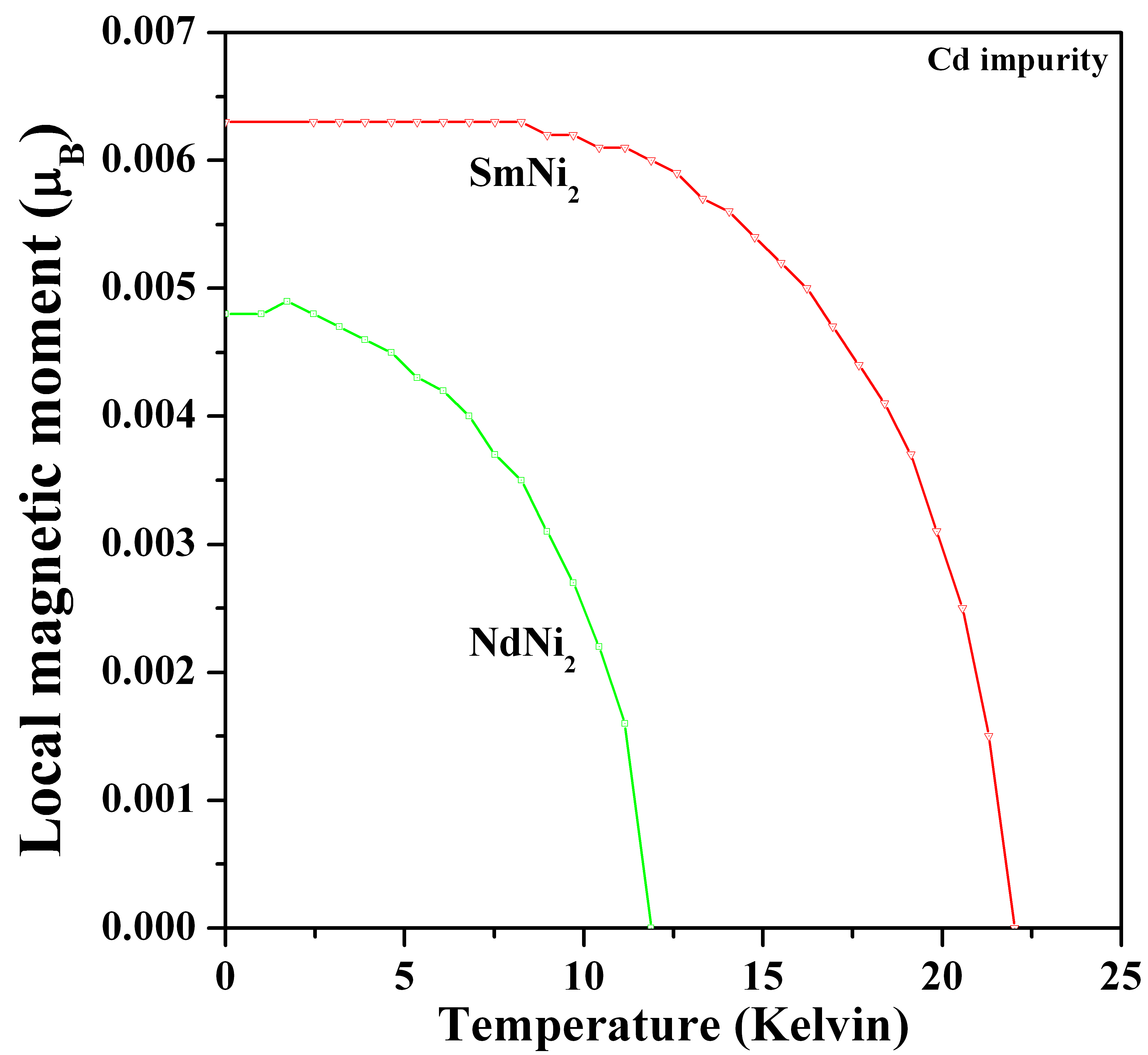
Figure 1: Local magnetic moment at Cd impurity diluted in $R$Ni₂ intermetallic host for light rare earths.

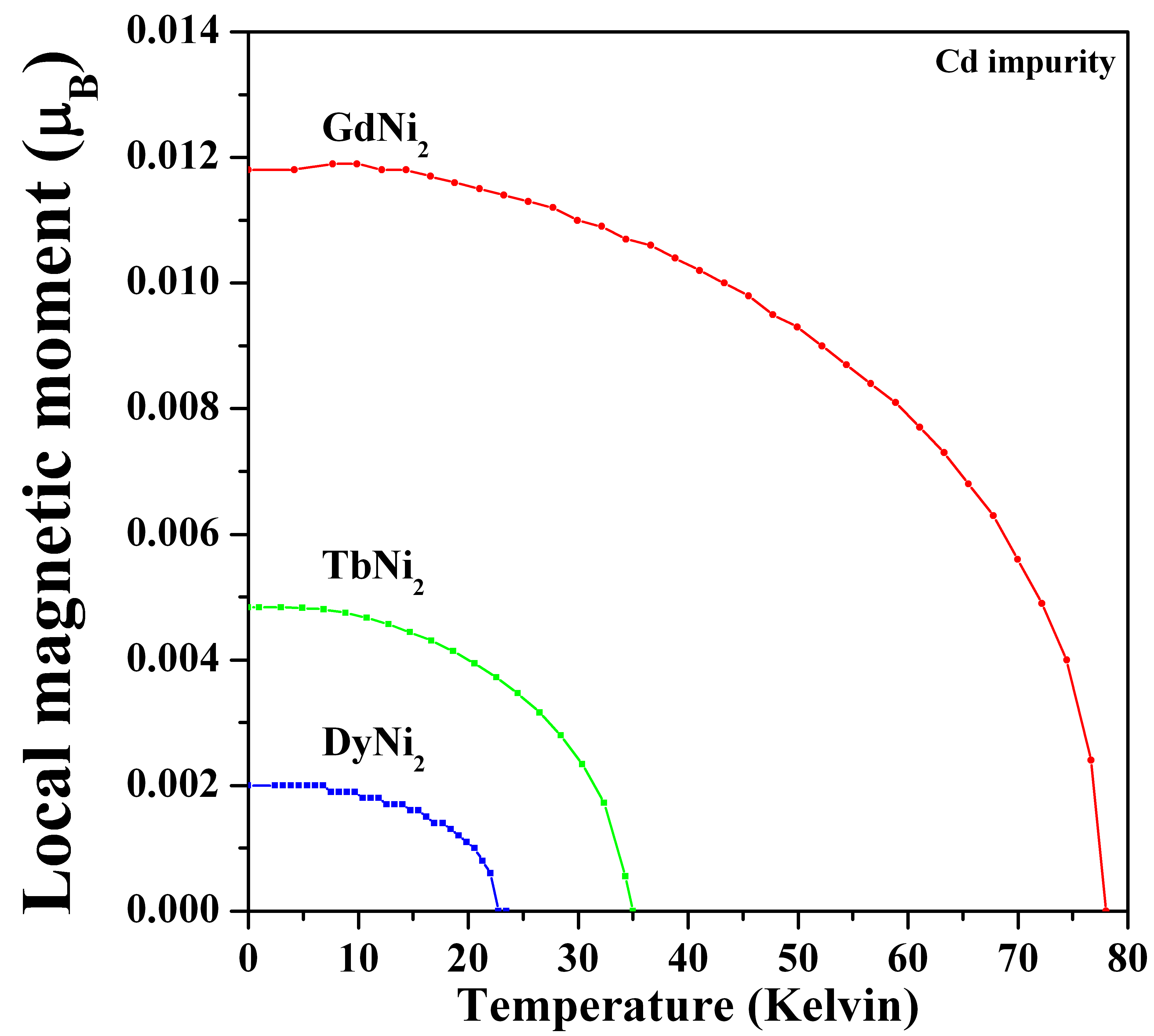
Figure 2: Local magnetic moment at Cd impurity diluted in $R$Ni₂ intermetallic host for heavy rare earths.

III Results and Discussions

We have introduced an effective model to extend our previous zero temperature results Oliveira2003 to investigate the magnetic hyperfine fields at a s-p impurity such as Cd, in $R$Ni₂ at finite temperatures. We adopt a standard paramagnetic density of state extracted from first principle calculation  Yama . For each $R$Ni₂ compound our model has two adjustable parameters, namely $\varepsilon_{0\sigma}$ and $U$. These are determined by reproducing the zero temperature local magnetic moment and the critical temperature.

In Fig. 1 , Fig. 2 and Fig. 3 we plot the calculated temperature dependence of the local magnetic moments for the light rare earth elements, for the heavy elements and the magnetic hyperfine fields at Cd as function of temperature.The results are good agreement with the experimental results Muller2004 .

As stated before, in the effective $R$ lattice the interactions are different from a $R$ pure metal. From Fig. 2 we see that the local moment, in units of Bohr magneton $\mu_{B}$, at $T=0K$ is about 0.012 whereas in Ref. alekos, it was found that in pure Gd metal it is about 0.05.

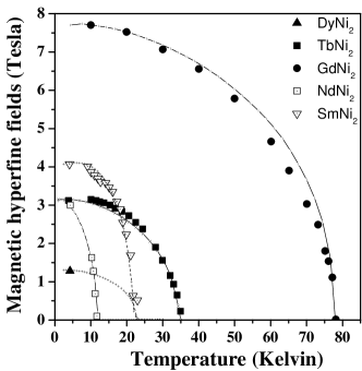
Figure 3: Magnetic hyperfine field at Cd impurity diluted in $R$Ni₂ intermetallic host. The experimental data were collected from Ref. Muller2004, .

References

• (1) K.H.J. Buschow. Rep. Prog. Phys., 40, 1179, (1977).
• (2) J. Hubbard, Phys. Rev. Lett. 3,77 (1959).
• (3) H. Hasegawa, J. Phys. Soc. Japan 46, 1504 (1979).
• (4) Y. Kakehashi, Phys. Rev B41, 9207 (1990).
• (5) B. VelickΓ½, S. Kirkpatrick, and H. Ehrenreich, Phys. Rev. 175, 747 (1968).
• (6) H. Hasegawa, J. Phys. Soc. Jpn. 49, 963 (1980).
• (7) I.A. Campbell, J. Phys. C 12, 1338 (1969).
• (8) A.L. de Oliveira, N.A. de Oliveira and A. Troper, Phys. Rev. B 67, 12411 (2003).
• (9) H. Yamada, J. Inoue, K. Terao, S. Kanda and M. Shimitzu, J. Phys. F: Met. Phys. 14, 1943 (1984)
• (10) S. MΓΌller, P. de la Presa and M. Forker, Hyperfine Interac. 158, 163 (2004).
• (11) A. L. de Oliveira, M. V. Tovar Costa, N. A. de Oliveira and A. Troper, J. Appl. Phys. 81,4215 (1997).