Long-term monitoring of the archetype Seyfert galaxy MCG-6-30-15: X-ray, optical and near-IR variability of the corona, disc and torus.

Abstract

We present long term monitoring of MCG-6-30-15 in X-rays, optical and near-IR wavelengths, collected over five years of monitoring. We determine the power spectrum density of all the observed bands and show that after taking into account the host contamination similar power is observed in the optical and near-IR bands. There is evidence for a correlation between the light curves of the X-ray photon flux and the optical B-band, but it is not possible to determine a lag with certainty, with the most likely value being around zero days. Strong correlation is seen between the optical and near-IR bands. Cross correlation analysis shows some complex probability distributions and lags that range from 10 to 20 days, with the near-IR following the optical variations. Filtering the light curves in frequency space shows that the strongest correlations are those corresponding to the shortest time-scales. We discuss the nature of the X-ray variability and conclude that this is intrinsic and cannot be accounted for by absorption episodes due to material intervening in the line of sight. It is also found that the lags agree with the relation $\tau\propto\lambda^{4/3}$, as expected for an optically thick geometrically thin accretion disc, although for a larger disc than that predicted by the estimated black hole mass and accretion rate in MCG-6-30-15. The cross correlation analysis suggests that the torus is located at $\sim 20$ light-days from the central source and at most at $\sim 50$ light-days from the central region. This implies an AGN bolometric luminosity of $\sim 3\times 10^{43}$ ergs/s/cm².

1 Introduction

One of the defining characteristics of Active Galactic Nuclei (AGN) is their strong variability, which is observed on time scales of seconds to years, and over a very broad wavelength range. The often complex, yet evident connection between the variations seen at different wavelengths has also been firmly established. These can be used to unveil the physical processes behind the emission and the relations between the different regions responsible for the variations, such as the corona (producing the X-ray emission), the accretion disc (producing the UV, optical and likely near-IR emission) and the dusty torus (producing near and mid-IR emission).

Multiwavelength, high quality light curves, (i.e., those with the desired energy coverage and time sampling), are not easy to obtain. The advent of current and future time domain surveys are helping to overcome this at least partially, yielding well sampled light curves for a huge number of sources, but usually limited to the optical band. Hence, multiwavelength monitoring data are still obtained from targeted observations of AGN from space and ground facilities, and it will remain this way for the time being.

The emerging picture from the analysis of long term, well sampled, multiwavelength observations of AGN is clear in its most simple version: variation patterns can be mapped at different wavelengths and observed lags are roughly consistent with the time it takes for radiation to travel from the center to the edges of the system. This confirms the expected temperature stratification, with the hot corona encompassing only a few gravitational radii ($R_{g}=GM/c^{2}$, where M is the black hole mass) around the black hole, the accretion disk extending from close to the location of the corona to hundreds or thousands of $R_{g}$, and the dusty torus appearing at the radii where dust can survive the prevailing temperatures (Suganuma et al. 2006; Arévalo et al. 2009, 2009; Breedt et al. 2009, 2010; Lira et al. 2011; Cameron et al. 2012; McHardy et al. 2014; Shappee et al. 2013; Edelson et al. 2015). The details, however, are still somewhat murky, which is not surprising as these are most likely function of several parameters such as black hole mass, accretion rate, system geometry and inclination, etc., which are bound to change from source to source, while for a single source, the accretion rate might change from one observation to the next.

MCG-6-30-15 is one of the best studied AGN in X-rays (Arévalo et al., 2005; McHardy et al. 2005; Miniutti et al. 2007; Miller et al., 2008, 2009; Chiang & Fabian 2011; Emmanoulopoulos et al. 2011; Noda et al. 2011; Marinucci et al. 2014; Kara et al. 2014; Ludlam et al. 2015; just to name some of the articles from the last 10 years). The interest in its X-ray emission is due to the presence of the broad red-shifted K$\alpha$ line, indicating X-ray reflection from the innermost region of the accretion disc (Tanaka et al. 1995), and its high variability (as first reported by Pounds et al. 1986 and Nandra et al. 1990), as expected from accretion onto a black hole of only a few million solar masses (Done & Gierlinski 2005; Ludlam et al. 2015). Indeed, MCG-6-30-15 is usually defined as a member of the Narrow Line Seyfert 1 (NLS1) class.

However, no monitoring campaign has aimed at longer wavelengths. In fact, to our knowledge, no reverberation campaign has been successfully carried out on this source and black hole mass estimates rely on the galactic properties of its host galaxy and X-ray variability derivations (McHardy et al. 2005 and references therein).

We wanted to remedy this situation by conducting a long monitoring campaign of MCG-6-30-15 from the X-rays to the near-IR wavelengths. This very broadband approach will give us an understanding of the relation between the corona, disc and torus components in this AGN. This paper is organised as follows: Section 2 presents the data acquisition and reduction; Section 3 presents the results on the determination of the Power Spectral Density, the Cross Correlation analysis and the frequency filtered light curves; Section 4 presents a discussion on the nature of the X-ray emission, the near-IR emission from the disc and torus and an upper limit to the bolometric luminosity of MCG-6-30-15; Section 5 presents the summary. Throughout this work we assume a distance to MCG-6-30-15 of 37 Mpc (z=0.008, Ho=65 km/s/Mpc).

2 Data acquisition and analysis

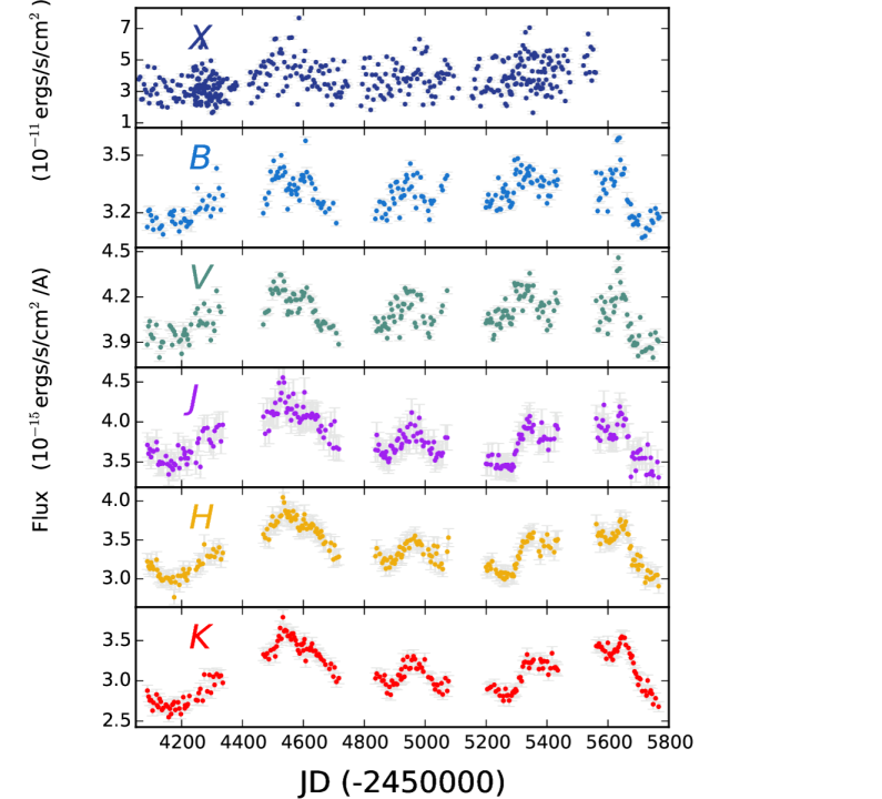
Figure 1: Observed X-ray, optical and near-IR light curves for MCG-6-30-15. Observations have not been corrected for host contribution or intrinsic extinction.

We monitored MCG-6-30-15 in the X-ray band with the Rossi X-ray Timing Explorer (RXTE) taking 1 kilo-second exposure snapshots typically every 4 days, but including some intensive periods with snapshots every 1 or 2 days. In the present paper, we include the X-ray data that are contemporaneous to our ground based observations (see below). The X-ray data were obtained using the RXTE Proportional Counter Array (PCA), which is sensitive in the range 3 to 60 keV and consists of five Proportional Counter Units (PCUs). We only extracted data from PCU 2. We use standard good-time interval selection criteria. Background data were created using the combined faint background model and the SAA history. We extracted spectra in the 3-–12 keV energy range for each snapshot and used XSPEC to fit a simple absorbed power-law model with the absorption column fixed at the Galactic value, $N_{H}=4\times 10^{20}$ cm^-2 to obtain an estimate of the 2–-10 keV flux and its error. For further details on data reduction of RXTE observations see Arévalo et al. (2008).

B, V, J, H, and K observations were obtained between August 2006 and July 2011 with the ANDICAM camera mounted on the 1.3m telescope at CTIO and operated by the SMARTS consortium. ANDICAM allows simultaneous observations in the optical and near-IR by using a dichroic with a CCD and a HgCdTe array. A movable mirror allows dithering in the IR while an optical exposure remains still. The average sampling of the light curves was 4.5 days.

The optical data reduction followed the usual steps of bias subtraction and flatfielding. The images were convolved to match the point spread function of the worst acceptable seeing. Relative photometry of MCG-6-30-15 and nearby stars was achieved by obtaining aperture photometry with a radius of 1.7 arcseconds. The final flux calibration was determined by observing standard photometric stars during photometric conditions. The data were corrected for Galactic foreground absorption of $A_{V}=0.165$. For more details on the optical data reduction see Arévalo et al. (2009).

The near-IR data reduction followed the standard steps of dark subtraction, flat fielding, and sky subtraction using consecutive jittered frames. The light curves were constructed from relative photometry obtained through a fixed aperture with diameter 2.74 arcsec after all images were taken to a common seeing. Flux calibration was obtained using the computed 2MASS magnitudes of the comparison stars. Photometric errors were obtained as the squared sum of the standard deviation due to the Poissonian noise of the source-plus-sky flux within the aperture, plus the uncertainty due the measurement itself. This last error was estimated as the standard deviation in the photometry of stars available in the field of view in consecutive exposures. For more details see Lira et al. (2011).

Light curves in the X-ray, B, V, J, H, and K bands for MCG-6-30-15 are presented in Figure 1.

3 Results

3.1 The Power Spectral Densities

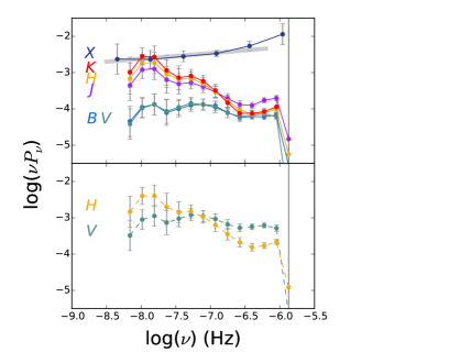
Figure 2: Top panel: Power spectral densities (PSDs) obtained from the X-ray, optical and near-IR observations for MCG-6-30-15. We also include the low-frequency slope previously fitted to the RXTE/XMM-Newton X-ray PSD by McHardy et al. (2005 – thick gray line). Lower panel: PSDs for the V and H bands after correcting for host contribution (see text for details).

We obtained the power spectral density (PSD) for all bands calculated using the Mexican hat filter method described in Arévalo et al. (2012). The Poisson noise contribution was estimated from the errors on the fluxes by simulating an error light curve of Gaussian deviates with zero mean and standard deviation equal to the error in each flux point. The power spectrum of these error light curves was calculated with the same method used for the real light curves and was subsequently subtracted from the total power spectrum. Error bars on the power spectra represent the expected scatter for different realizations of a red-noise process. For highly correlated energy bands (such as B and V bands) this error overestimates the band to band scatter.

In order to combine the RXTE long time scale and XMM short time scale observations, we followed McHardy et al. (2005, 2004), and restrict the energy range of the XMM light curve to 4-10 keV, whose mean photon energy match well the 2-10 keV mean energy of a photon from RXTE.

Aliasing from higher frequencies can be important in the X-ray power spectrum, since its break timescale is about 4 hours (McHardy et al. 2005) and the observations are on average taken 4 days apart, i.e., there is significant variability power on timescales much shorter than those sampled. To estimate the effect of aliasing on the X-ray power spectrum we simulated X-ray light curves with the power spectral parameters given in McHardy et al. (2005): a broken power law ($P_{\nu}\propto\nu^{\alpha}$) with slopes $\nu_{L}=-0.8$ and $\nu_{H}=-2.5$ at low and high frequencies, break frequency of $7.6\times 10^{-5}$ Hz, and using a generation bin size of 0.01 days. We resampled these simulations to match the sampling of the real light curve and calculated the power spectrum with the same method used for the real data. The median power spectrum of 100 trials was fitted with a power-law of free slope and normalization in the range $10^{-8}-2\times 10^{-6}$ Hz. We varied the input low-frequency slope around the best fitting value and obtained flatter but comparable slopes in the resulting power spectra, as expected from the effect of aliasing. For input slopes of 0.9, 0.85 and 0.8, the measured slopes were 0.8, 0.76 and 0.69, respectively. The real X-ray lightcurve gave a slope of 0.74, which is consistent with an intrinsic slope of 0.85, similar to the value obtained from a different data set by McHardy et al. (2005). Aliasing is much less important in the optical and IR bands, where the sampling rate is sufficient to track the major flux variations.

Figure 2 presents the PSDs for all bands. Clearly, all the PSDs present a rather flat distribution in units of $\nu\times P_{\nu}$, which is recognized as the self-similar flicker-noise region of the PSD (e.g. Uttley 2007). The inverted (positive in $\nu\times P_{\nu}$ units) slope of the X-ray PSD was already seen by McHardy et al. (2005), as discussed above. We have included the low-frequency slope fitted by McHardy et al. (2005) in Figure 2. Our PSD slightly extends the low frequency coverage down to $5\times 10^{-9}$ Hz. No sign of a secondary break is seen, as expected from observations of other low black hole mass AGN and black hole X-ray binaries in the soft state (Done & Gierlinski 2005; Uttley 2007).

The PSDs of the longer wavelength bands show clearly less power than that seen in the X-rays. Interestingly, the near-IR PSDs have more power than those of the B and V bands, except at frequencies above $\sim 5\times 10^{-7}$ Hz where the power becomes comparable. However, the host galaxy makes a non-negligible contribution to the optical and near-IR bands, adding to the total flux but not to the fractional flux variations, therefore decreasing the amplitude in the observed variability and diminishing the power in the PSD (notice that extinction, being a multiplicative factor, does not change the obtained PSD; e.g. Uttley et al. 2002). We can assess this correction using the H-band IFU SINFONI data recently presented by Raimundo et al. (2013). They find that the total emission within a circular aperture with diameter 3 arcsec (very close to the aperture used to determine our light curves) corresponds to $f_{H\star}\sim 3.4\times 10^{-15}$ erg/s/cm²/Å (in very good agreement with the mean value of our light curve), of which $\sim 45\%$ corresponds to the underlying stellar population (Raimundo, private communication).

Extrapolating to the optical region is not straightforward, as we need to assume a spectral energy distribution for the stellar population. On the one hand, the S0 nature of the MCG-6-30-15 host might argue for a rather old population. However, based on the presence of FeII emission lines in the H-band spectra, Raimundo et al. (2013) argue for the presence of a nuclear cluster with a stellar age of $\sim 10^{8}$ years. For such a young stellar population the contribution to the V-band will be $\sim 10$ times larger than that observed in the H-band, i.e., $f_{V\star}^{0}\sim 1.5\times 10^{-14}$ erg/s/cm²/Å, which translates onto $f_{V\star}\sim 2.7\times 10^{-15}$ erg/s/cm²/Å for an extinction of $E(B\!-\!V)=0.6$ (Reynolds et al. 1995), below the minimum level seen in our V-band light curve.

The bottom panel in Figure 2 presents the V and H corrected PSDs after subtracting the host contribution in both bands. It can be seen that the two PSDs have now a similar power level, and that they might cross somewhere between $10^{-7.5}$ and $10^{-7.0}$ Hz, but the differences are within one sigma errors and the scaling of the PSDs is very sensitive to the host correction just introduced, which is not well known. Still, it is interesting that the near-IR bands show such a large amount of variability power when compared with the optical, since disc variability is expected to decrease at larger radii.

In some more detail, note that around $10^{-8.0}$ Hz or 2 years the uncorrected K-band has comparable power to the X-ray band, but galactic contamination is probably negligible at X-ray energies, so this power spectrum gives a good estimate of the true fractional X-ray variability. The K-band, on the other hand, contains some level of stellar contamination, and therefore the AGN fractional variability in this band can only be corrected upwards. Finally, the V-band variability does not reach these high powers even after correcting for stellar contamination. The large amplitude of the K-band fluctuations can be interpreted as reprocessed thermal emission from the torus. Since this structure does not have and internal source of heating, it can only respond to the optical, UV and X-Ray continua emitted by the disc and corona. The long term K-band variations in MCG-6-30-15 are as large as those of the X-Rays and could also be responding to the (unobserved) UV, but the optical power seems to be insufficient to drive the near-IR variability.

3.2 Correlation Analysis

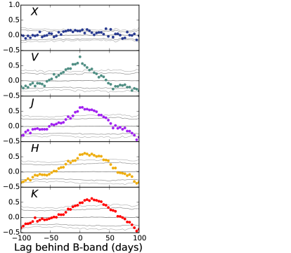
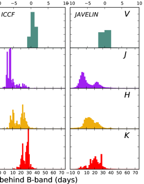
Figure 3: Left: Correlation coefficient from CDF analysis between the B band and all other observed bands for MCG-6-30-15. Positive lags mean that the annotated band lags behind B. The continuous gray lines represent the mean, 95% and 99% upper and lower confidence limits. Right: DCF, ICCF and JAVELIN centroid distributions between the B band and all other optical and NIR observed bands. As before, positive lags mean that the annotated band lags behind B. Notice the different axis ranges for the top panels.

Table 1: Results from the correlation analysis of the full and filtered light curves. Lags are measured with respect to the B band and are expressed in days. A positive lag means the B band leads the variability. JAVELIN $1\sigma$ confidence limits and centroids for the discrete correlation functions (DCFs) and interpolated cross correlation functions (ICCF) are presented. ICCF centroids are determined at a $1\sigma$ level. DCF lag centroids measured at a 95% confidence level are denoted with a star while other lags are determined at a 99% confidence level.

	Javelin Full	ICCF Full	DCF Full	DCF $k1$	DCF $k2$	DCF $k3$	DCF $k4$
V	0.0 : 1.8	$-0.7\pm 2.2$	$-0.4^{+2.1}_{-3.0}$	$-8.2^{+3.1}_{-2.9}$	$-5.3^{+4.0}_{-3.9}$	$-3.8^{+1.9}_{-1.8}$	$-1.8^{+1.3}_{-0.6}$
J	4.1 : 25.0	$13.5\pm 4.3$	$11.0^{+3.0}_{-2.9}$	—	$10.0^{+3.3}_{-3.3}$	$9.5^{+2.2}_{-2.6}$	$10.3^{+2.1}_{-1.9}$
H	8.6 : 25.1	$20.0\pm 4.0$	$16.7^{+3.7}_{-4.2}$	—	$\star 17.6^{+3.9}_{-3.9}$	$13.6^{+2.8}_{-1.9}$	$17.0^{+3.3}_{-4.4}$
K	6.9 : 29.3	$26.1\pm 3.7$	$18.5^{+3.8}_{-3.6}$	—	$\star 16.2^{+4.4}_{-4.1}$	$18.0^{+3.4}_{-3.4}$	$19.8^{+2.1}_{-2.2}$

From Figure 1 it can immediately be seen that a high degree of flux correlation exists between the optical and the near-IR, with the short term variability gradually diminishing in significance towards longer wavelengths. No correction for host galaxy contamination is introduced. Therefore the overall observed amplitudes of the light curves should be regarded as a lower limit to the real variations.

We have quantified the degree of correlation between bands using three methods: the discrete correlation function (DCF) of Edelson & Krolik (1988) with confidence limit determinations following Timmer & Konig (1995), the interpolated cross correlation function (ICCF) presented by Peterson et al. (1998, 2004), and the JAVELIN cross-correlation method of Zu et al. (2011, 2013), which models the light curves as a damped random walk process (DRWP) as prescribed by Kelly et al. (2009). While the DCF method does not require any assumption about the the variability to work, the Timmer & Konig (1995) technique to derive its significance requires a previous knowledge of the shape of the PSD in order to simulate synthetic light curves (see below). On the other hand, the ICCF is a model-independent estimate of the degree of correlation. Finally, JAVELIN assumes a particular regime of the PSD (a DRWP or $P_{\nu}\propto\nu^{\alpha}$ with $\alpha=-2$, breaking to $\alpha=0$ at a characteristic frequency) in order to determine a lag and its significance. No host correction has been introduced to the light curves during the cross-correlation analysis using either of the described methods.

We determined the DCFs for the year-long segments of the RXTE and optical–near-IR light curves and then combined them. In Figure 3 we present the DCFs obtained between the B-band and all other observed bands, with 95% and 99% confidence limits following Timmer & Konig (1995), i.e., by determining the cross correlation of the observed B-band light curve and a synthetic light curve of the band of interest simulated according to the power law shape of its PSD. This process was repeated 1000 times and the DCF distributions obtained were used to determine the confidence limits. The lags corresponding to the main peak in the DCF distributions were estimated using the random sample selection method of Peterson et al. (2004), selecting 68 percent of the data points in the B and near-IR light curves and calculating the DCF centroid for 1000 such trials. The resulting centroid distributions are also shown in Figure 3 and their mean values and errors are presented in Table 1. Further details of the procedure can be found in Arévalo et al (2008).

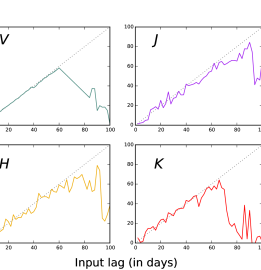
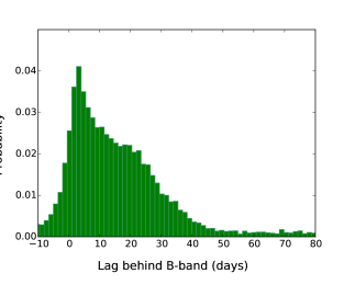
Figure 4: Top: JAVELIN results for the cross correlation between the observed B-band light curve and the shifted V, J, H and K-bands after randomization was applied. See text for details. Bottom: JAVELIN lag distribution for simulated B and J light curves generated as described in the text.

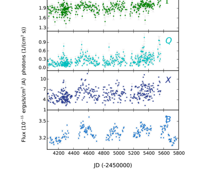
Figure 5: $\Gamma$, X-ray photon flux (Q), X-ray flux and B-band flux light curves for MCG-6-30-15.

ICCF results for the same RXTE and optical–near-IR light curves were determined using a grid of 1 day for the interpolation of the data before determining the cross-correlation. For the calculation of the lag and its uncertainty, interpolated, bootstraped data were cross-correlated and those results with correlation coefficients larger than 68% out of 1000 trials where used to find the median lag and its 1$\sigma$ confidence limits. The resulting centroid distributions are presented in Figure 3 and the measured mean lag are tabulated in Table 1.

For the JAVELIN analysis we followed Shappee et al. (2014) and Pancoast et al. (2014), and calculated the distribution of lags from 10000 Monte Carlo simulations for each separate segment and then combined the yearly probability distributions. From the resulting distributions 1$\sigma$ intervals were measured as the lag values that represented the 1-CL at each end of the distributions, with CL $=0.6827$. Results are presented in Figure 3 and Table 1.

A quick inspection of Figure 3 confirms that all three cross correlation methods, DCF, ICCF and JAVELIN, are consistent with each other, although the DCF centroid distributions show less structure than the distributions found from the JAVELIN and ICCF analysis. Interestingly, the J and H bands present some evidence of double peaks in their distributions, as can be seen in the ICCF and JAVELIN results. This could be a sign for more than one lag present in MCG-6-30-15, as will be discussed in more detail in Section 4.2.

Assuming a DRWP as a good description of the observed light curves, however, might not be appropriate for our study. While DRWP is characterised by $P_{\nu}\propto\nu^{-2}$, breaking to $P_{\nu}\propto\nu^{0}$ at lower frequencies, it is clear that our X-ray PSD is better characterised by $\alpha>-1$ and the optical PSDs are more consistent with a power distribution given by $\alpha\sim-1$ (see Figure 2). The near-IR bands, on the other hand, seem more consistent with a random walk process. We expect, however, that the near-IR variability might be the combination of variations coming from two structures, the disk plus the torus, making the DRWP assumption also flawed.

To assess this issue we used JAVELIN to determine the lag between the B-band and the V, J, H and K-bands after these were shifted back to zero lag using the DCF results reported in Table 1, and then shift them forwards up to a lag of 100 days using a step of 2 days. For each calculation, the curve of interest was randomized in its flux assuming Gaussian distributed errors, and in time, by shifting the date assuming a flat probability with a width of 10% around the actual observing date. The results are presented in Figure 4. The plots show that the output lags are strongly under-predicted for delays longer that 50 days, but that they can recover input lags before that. Since all of our findings report lags much shorter than this our JAVELIN results should be correct. This is also supported by the similar behaviour shown by the JAVELIN results and those from the DCF and ICCF analysis.

In order to investigate whether JAVELIN is indeed able to determine the presence of more than one lag during the cross-correlation analysis we performed the following test: B and J-band in-phase synthetic light curves were computed assuming PSDs with slopes of -1 and -2, similar to the observed values, and break frequencies at 100 and 1000 days, respectively. This ensures that both light curves are coherent, but with the J-band light curve being much smoother than the B-band light curve. Next, two versions of the J-band light curves are computed applying a lag of 5 and 20 days and their average is determined. The resulting JAVELIN lag distribution between the B-band and the linearly combined two-lag J-band light curves can be seen in Figure 4. Clearly, there is evidence for a double peak consistent with the lags introduced in the synthetic light curves. To find what combination of parameters would yield results similar to those presented in Figure 3 is beyond the scope of this paper.

From the X-ray and B-band DCF plot in Figure 3 it can be seen that no significant correlation signal is found. JAVELIN analysis did not give a clear result (plot is not shown) which could be related to the problem of adopting a DRWP as a description of our X-ray observations.

The DCF result is not totally unexpected as the X-rays show very fast variability and our RXTE and optical–near-IR light curves are not suitable to determine a correlation between these bands. A correlation was previously determined between the X-ray emission and the 3000–4000 Å U-band of the Optical Monitor on-board XMM-Newton (Arévalo et al., 2005). The observations corresponded to snapshots 800 seconds long separated by gaps of 320 seconds. Such fast monitoring allowed us to determine a lag of $1.85^{+0.52}_{-0.75}$ days, with the U-band leading the X-rays. In that case the X-ray light curve tracked lower energies since the bulk of the photons recorded by the XMM pn camera are below the 2 keV threshold of RXTE and are therefore dominated by the soft excess present in MCG-6-30-15. In fact, the soft excess has been shown to correlate better with the optical bands than the hard X-rays in at least one source with good quality UV, soft and hard X-ray light-curves (Mrk509; Mehdipour et al. 2011). In fact, a re-analysis of the XMM-Newton data by Smith & Vaughan (2007) did not report a significant lag. Smith & Vaughan (2007) argue that the differences with Arévalo et al. (2005) are due to the different methods used to extract the light curves and a more conservative treatment of the correlation analysis.

We also obtained the cross correlation between the B-band and the X-ray photon flux light curve, Q, which is presented in Figure 5. In the framework where the corona is cooled by Comptonization of (the unseen) UV and optical photons, significant changes in the UV/optical flux should be correlated with changes in the X-ray flux. However, the corona energetics also respond to changes in the UV/optical flux, with higher fluxes inducing more efficient electron cooling. This in turn will mean that B-band photons will gain less energy from the corona and therefore the shape of the X-ray spectrum will become steeper. This trend is seen in Figure 5, where the photon index $\Gamma$ of the 3-10 keV energy range (i.e., for flux $\propto\nu^{-\Gamma}$ photons/s/cm²) grows steadily during the monitoring from a value of $\sim 1.8$ at the start of the campaign to $\sim 2.0$ towards the end.

As shown by Nandra et al. (2000), in cases of a variable $\Gamma$ it is expected that the photon flux Q would be more closely correlated with the UV or optical flux, because of the one-to-one nature of the Compton scattering between photons and electrons. In Figure 6 we present the cross correlation between Q and the B-band obtained using the DCF and the ICCF methods. As can be seen, there is good evidence for a correlation with a lag around zero. Unfortunately, the centroids are found with very large spreads of $8^{+6}_{-48}$ and $2.1\pm 20.1$ days for the DCF and ICF methods, respectively, with the Q-band leading. The correlation, however, is present, with a 100% of the (1000) centroid calculations performed during the ICCF trials being successful and a mean peak correlation coefficient of $0.48\pm 0.04$.

On the other hand, there is a clear correlation signal between the near-IR bands and the optical bands. The rather flat near-IR DCFs in Figure 3 resemble those of NGC 3783, where a very broad and flat correlation was interpreted as resulting from the sum of two variable components varying on different time scales: a rapidly varying disc and slower dusty torus (Lira et al., 2011).

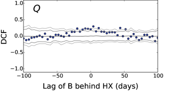
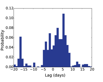
Figure 6: Top: Cross corelation between the Q and B-band from the DCF. Bottom: Cross corelation between the Q and B-band from the ICCF.

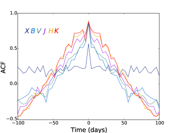
Figure 7: Auto correlation functions (ACFs) of all the light curves presented in Figure 1. From the inner-most to the outer-most curves, the ACFs correspond to the X, B, V, J, H and K-bands.

We can test the presence of more than one component by comparing the width of the auto correlation functions (ACFs) in different bands. If one band drives the variability in the remaining bands, then it is expected that its ACF should be the narrowest, with the remaining band ACFs been broadened by the response of the system. Long time responses will correspond to broad ACFs, and most likely, to more extended emitting regions. The X-ray, B, V, J, H and K-band ACFs are presented in Figure 7. As can be seen, there is a systematic broadening of the ACFs when going from the shortest to the longest wavelengths, with the X-ray ACF been particularly sharp and narrow. At the same time, the ACFs of the B and V bands are very similar, while the H and K ACFs also look very much alike and are clearly the broadest of all. This might indicate the presence of a large reprocessor, like the dusty torus, significantly contributing to the variability in the H and K bands.

The ICCF and JAVELIN results for the J, H and possibly the K-band are complex and hint at the presence of more than one distinct variable component. In fact, the centroid values presented in Table 1 should be considered as a poor representation of the multiple peaks observed.

3.3 Filtered Light Curves

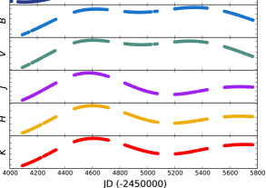
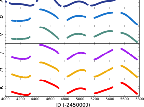
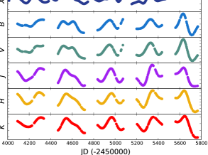
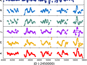
Figure 8: Filtered light curves for the X-ray, B, V, J, H, and K bands, and for frequency ranges $k1=7\!\times\!10^{-9}\!-2\!\times\!10^{-8}\!$ Hz, $k2=2\!\times\!10^{-8}\!-6\!\times\!10^{-8}\!$ Hz, $k3=6\!\times\!10^{-9}\!-2\!\times\!10^{-7}\!$ Hz, and $k4=2\!\times\!10^{-7}\!-6\!\times\!10^{-8}\!$ Hz.

We filtered the optical and near-IR light curves using the method described by Arévalo et al. (2012). In short, the method consists of filtering the data using a ’mexican-hat’ filter which suppresses fluctuations with time scales much larger or much smaller than a characteristic time scale. The method is also able to deal with gaps in the data, which are masked out during the analysis. In our case we did not mask out any data but instead worked on year-long segments.

Four light curves were produced with characteristic frequency intervals of $k1=7\!\times\!10^{-9}\!-2\!\times\!10^{-8}\!$ Hz (560-1680 days), $k2=2\!\times\!10^{-8}\!-6\!\times\!10^{-8}\!$ Hz (186-560 days), $k3=6\!\times\!10^{-9}\!-2\!\times\!10^{-7}\!$ Hz (62-186 days), and $k4=2\!\times\!10^{-7}\!-6\!\times\!10^{-8}\!$ Hz (21-62 days). These intervals are equally spaced in log frequency and the light curves were determined applying the ’mexican-hat’ filter to the PSDs. Figure 8 shows the light curves obtained for all our bands for the four frequency ranges.

We determined the cross correlation of the filtered light curves using the DCF method. Unfortunately, it is not possible to apply the JAVELIN code in this case as the random walk modelling of the light curves is only valid when describing the full data. As before, no significant cross correlation results were obtained for the X-ray filtered curves and the optical or near-IR filtered curves.

Figure 9 shows the DCFs between the B and V, J, H and K bands corresponding to all the frequency ranges. Only upper 99% confidence limits are included in the plots this time. It can be seen that the level of significance of the DCFs is higher at higher frequencies. In particular the first frequency range, corresponding to $\sim 3$ years, which is hardly sampled by our monitoring programme, does not give significant lags for any of the near-IR bands. However, a significant lag can be measured for the V-band because of its extreme similar behaviour to the B-band. For the $k2$ frequency range the V and J bands show DCFs significant at the 99% level, while for $k3$ and $k4$ all DCFs are significant at this level. At a 95% significance level, all DCFs are significant for frequency ranges $k2$, $k3$ and $k4$. Centroids are presented in Table 1.

A quick examination of Table 1 shows that for a given frequency range the near-IR bands respond with characteristicly longer lags when going towards longer wavelengths (i.e., when reading the table vertically). For instance, the lag nearly doubles when going from the J to the K band for the $k3$ and $k4$ frequency ranges. At the same time there is no clear trend in the different lags for the same band measured at different frequency ranges (i.e., reading the table horizontally). So, for example, the J band has a lag consistent with $\sim 10$ days for all frequency ranges, while the K band hints at lags that increase monotonically from $k2$ to $k4$. This implies that the reprocessor is responding equally at all time scales, and the lags only depend on the observed band.

Because of the similar variability pattern observed in the B and V bands, the cross-correlations of their frequency filtered light curves show larger correlation coefficients and smaller lag errors than those obtained in the near-IR. It is possible, then, to look at some trends that the lags exhibit with frequency. First of all, it can be noticed that all the lags determined using the DCF method are negative and that the values become more negative towards lower frequencies. This is likely due to contamination of emission from the Broad Line Region (BLR) to our optical photometry. The strongest line in the wavelength range covered by our observations ($\sim 3900-5900$ Å) is H$\beta\lambda 4861$, which falls in B-band filter. This would explain why the lag gets shorter with increasing frequency range, as the component from the slowly varying BLR will be more pronounced in the $k1$ than in the $k4$ light curve. Notice also that the full light curve shows the shortest lag. This is likely because the frequency ranges examined leave out a large fraction of the variability power seen in the optical, which concentrates at shorter frequencies than those found in the $k4$ range.

Since there is very little line contamination in the V-band we conclude that the B-band light curve is delayed. However, given the small negative lag measured from the cross correlation of the full light curves ($-0.4^{+2.1}_{-3.0}$ and $-0.7\pm 2.2$ days for the DCF and ICCF analysis, respectively, see Table 1), we will not attempt to correct for this effect.

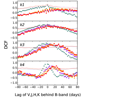
Figure 9: Correlation coefficients from DCF analysis between the B and VJHK bands for MCG-6-30-15 from the lowest (top) to the highest (bottom) frequency ranges. The solid lines represent the 99% colour-coded upper confidence limits for the different DCFs.

4 Discussion

4.1 The nature of the X-ray variability

The presence of the broad Fe K$\alpha$ line in the X-ray spectrum of MCG-6-30-15 has made this object one of the most intensively studied AGNs in the sky. Modelling of this feature as a gravitationally redshifted line scattered off hot, optically thick material located at a distance below $10R_{g}$ from the central black hole provides some of the best evidence for the presence of an accretion disc and opens the possibility of studying the behaviour of matter and radiation in a strong gravity environment (e.g., Tanaka et al. 1995; Iwasawa et al. 1996; Guainazzi et al. 1999; Lee et al. 1999; Vaugh & Edelson 2001; Wilms et al. 2001; Fabian et al. 2002; Shih et al. 2002; Fabian & Vaughan 2003; Marsumoto et al. 2003; Vaughan & Fabian 2004; Miniutti et al. 2007; Kara et al. 2014).

However, some authors have also proposed alternative models where the line can be explained by the presence of a continuum affected by complex absorption by ionized material, or a ’warm absorber’ (Inoue & Matsumoto 2003; Miller, Turner & Reeves 2008, 2009). Crucially for our study, using a warm absorber composed of several zones with varying partial covering of the central source, Miller, Turner & Reeves (2009) and Miyakawa et al. (2009) propose to explain not only the X-ray spectrum of MCG-6-30-15, but also most of its variability.

However, there is one piece of evidence that argues against the above scenario and that we can explore here: the rms-flux relation of the X-ray emission. Uttley & McHardy (2001) and Uttley et al. (2005) have demonstrated the non-linear nature of the X-ray variability in AGN. In fact, they show that variability is a multiplicative process, while additive processes, such as the combination of independent occultation episodes, can be ruled out. Empirically, this translates into the ’rms-flux’ relation. In other words, the multiplicative nature of the variability predicts a linear correlation between the flux level and its standard deviation.

Using a long look observation of MCG-6-30-15, Vaughan et al. (2003), already presented a clear ’rms-flux’ linear correlation for this source. We have combined our RXTE observations with those presented in McHardy et al. (2005) post year 2000, and new XMM observations (Marinucci et al. 2014; Kara et al. 2014) with those previously presented in Vaughan et al. (2003) to determine two ’rms-flux’ plots, following the method of Vaughan et al. (2003). Since the temporal resolution of the RXTE and the XMM observations are very different, each plot presents the results for each space-craft.

The XMM observations were binned into 100 second intervals, while the observing cadence of the RXTE light curves (approximately 2 and 4 days for the McHardy and our data, respectively) was not changed. The weighted mean flux and its standard deviation were determined from consecutive groupings of 15 bins each. To reduce scatter, further binning of 15 such flux-rms pairs was obtained. The results are presented in Figure 10 where the vertical “error” bars represent the scatter around a given rms value (i.e., they do not correspond to the error of the mean rms). The linear correlation is clear and we confirm that multiplicative nature of the X-ray variability in MCG-6-30-15 in both temporal regimes.

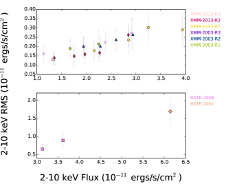
Figure 10: RMS-flux correlations for MCG-6-3015. Top: XMM-Newton observations obtained in 2001 and 2013. Each observation was divided into their individual XMM ’revolutions’. Bottom: RXTE observations obtained by McHardy et al. (2005) and this work.

4.2 Disc and torus variability at optical and near-IR wavelengths

The discrete correlation function between the B and the near-IR bands is seen in the left hand side of Figure 3. The DCFs show broad, flat-top peaks, which might suggest more than one variable component contributing to the signal. This has already been seen in NGC 3783 and interpreted as the disc and the dusty torus simultaneously contributing to the near-IR DCFs, with the disc dominating at smaller lags and the torus dominating at longer lags (Lira et al. 2011). The ICCF and JAVELIN results also suggest the presence of more than one component in the J and H-band lag probability distribution seen in the right hand side of Figure 3, and even perhaps in the K-band.

In the case of NGC 3783 the presence of the torus is also corroborated by a clear near-IR hump in its spectral energy distribution (Lira et al. 2011). Unfortunately, the very high extinction towards the nucleus of MCG-6-30-15 implies that the determination of its optical to near-IR spectral energy distribution is rather unfeasible. However, the H and K bands can give a good idea of the intrinsic spectral shape since they are less susceptible to extinction, and the stellar populations show a particularly homogeneous flux ratio between these two bands ($f_{H}/f_{K}\sim 2.5$), regardless of the stellar age. Adopting a stellar contribution of 45% in the H (see Section 3.1), a 18% K band contribution is then found. For $E(B-V)=0.6$, we find that absorption and host corrected H and K fluxes are $\sim 3.1$ and $3.5\times 10^{-15}$ ergs/s/cm²/Å, respectively, hinting at a red slope and therefore suggesting the presence of hot dust in the MCG-6-30-15 nuclear region.

We will attempt to isolate the emission from the disc from that from the torus by using the distinct ’disc’ peaks observed in the JAVELIN probability distributions, this is, the V peak and the first peaks seen in the J and H distributions. We will assume that the K-band JAVELIN main peak corresponds to a ’torus’ lag. By fitting a Gaussian to these features we were able to determine their characteristic centre and dispersion. The values are: V-disc-lag = $-0.8\pm 0.9$, J-disc-lag = $4.9\pm 3.8$ H-disc-lag = $11.4\pm 4.6$, J-torus-lag = $21.9\pm 4.2$, H-torus-lag = $22.1\pm 4.5$ and K-torus-lag = $19.6\pm 4.9$. These values suggests that the outer disc is truncated at distances $\ga 15$ light-days, with the torus appearing at $\la 20$ light-days.

In Figure 11 we present the JAVELIN ’disc’ lags determined as given above (blue circles), as a function of wavelength. The K-band JAVELIN ’torus’ lag is also included (red star). To test whether we are in fact seeing disc emission in the JAVELIN ’disc’ lags, we can look at the correlation of the lags with wavelength and see whether these are in agreement with the predicted relation $\tau\propto\lambda^{4/3}$ for the outward light travel time in an optically thick geometrically thin accretion disc.

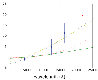
Figure 11: Observed and model lags as a function of wavelength. V, J and H ’disc’ lags were determined from the JAVELIN probability distributions and are shown as blue circles; the K-band ’torus’ lag is shown with a red star (see text for details). The blue dot-dashed line corresponds to the best fit assuming the functional form $\tau=A((\lambda/\lambda_{0})^{4/3}-1)+B$. The yellow dashed line corresponds to the best fit for a standard optically thick geometrically thin accretion disk model of the form $\tau=3\!\times\!10^{-10}\lambda^{4/3}\dot{m}^{1/3}M^{2/3}$, where $\dot{m}$ and $M$ are the accretion rate and black hole mass, which are left as free parameters. The best estimates of $\dot{m}$ and $M$ give the green solid line, which clearly under-predicts the observed lags. The red dotted line includes the effects of X-ray heating for a flared disc, as described in more detail in the text.

We determined a weighted fit to the JAVELIN V, H and J ’disc’ lags. Following Edelson et al. (2015), first we fit a function of the form $\tau=A((\lambda/\lambda_{0})^{4/3}\!-1)\!+B$, with $\lambda_{0}=4000$Å. The best fit requires $A=2.4$ and $B=-0.9$ and is presented as a blue dashed-dotted line in Figure 11.

A fit setting $B\!=\!0$ was done in a physically motivated way, as follows. We included the prescription for the light travel time across a standard optically thick geometrically thin accretion disk model of the form $\tau=3\!\times\!10^{-10}\lambda^{4/3}\dot{m}^{1/3}M^{2/3}$, for $\tau$ expressed in days and $\lambda$ in Å, and where $\dot{m}$ is the accretion rate in Eddington units and $M$ is the black hole mass in units of solar masses (e.g., Shakura & Sunyaev 1973). The green solid line in Figure 11 shows the predicted lags for $M=5\times 10^{6}$ M_☉ (McHardy et al. 2005) and $\dot{m}=0.04$ (see next section). Clearly, the lags are up to a factor 4 longer than predicted by the accretion model. A fit to the data leaving $\dot{m}$ and $M$ as free parameters yields $\dot{m}=0.2$ and $M=1.1\times 10^{7}$ M_☉, both much larger than the estimates, and is shown in Figure 11 with a yellow long dashed line.

Illumination or heating of the disc by the central X-ray emission can modify the disc temperature profile. Since the disc becomes hotter, a region emitting most of the radiation corresponding to a given wavelength will move outwards to larger radii. For a flared disc, the changes can be even more significant as a larger fraction of the X-ray flux is intercepted by the disc. Besides, it is easy to argue that it is just consistent to include heating from the central X-ray source when computing the $\tau\propto\lambda^{4/3}$ correlation: the cross correlation analysis clearly demonstrate that the observed lags are consistent with the light travel time across the system and that such a signal is propagating outwards; in other words, we see the disc being illuminated from the centre.

We follow Lira et al. (2011) and assume $M=5\times 10^{6}$ M_☉, $\dot{m}=0.04$, a 2-10 keV X-ray power of $7.0\times 10^{42}$ ergs/s (for a mean X-ray flux of $\sim 4\times 10^{-11}$ ergs/s/cm², as seen in our observations), a factor 2 to take the 2-10 keV X-ray luminosity to the the full 0.01-500 keV range, a disc innermost stable orbit at 3 $R_{g}$, a low disc albedo of 10%, a heavily flared disc with a power law profile of index 1.5 and characteristic radius $R_{0}$ of 100 $R_{g}$ (i.e., a disc height of the form $H\propto(R/R_{0})^{1.5}$), and a height of the X-ray source above the disc of 10 $R_{g}$. This predicts unreddened V-band fluxes $f_{V{\rm Grav}}=1.6\times 10^{-14}$ and $f_{V{\rm XR}}=4.1\times 10^{-14}$ ergs/s/cm²/Å due to the release of gravitational and X-ray heating, respectively. After an extinction of $E(B\!-\!V)=0.6$ is applied, this corresponds to $2.9\times 10^{-15}$ and $7.4\times 10^{-15}$ ergs/s/cm²/Å. Clearly, the predicted V-band flux due to X-ray heating is too large to account for our observations. If we take into account our (rather extreme) estimate of the host contribution to the V-band (see Section 3.1), then $f_{V\star}+f_{V{\rm Grav}}=5.6\times 10^{-15}$ erg/s/cm²/Å, about 35% above the observed mean flux value in the V-band light curve.

The predicted lags as a function of wavelength for the described disc model is plotted in Figure 11 with a dotted red line. As can be seen, even though the predicted lags are significantly increased at longer wavelengths, this effect is not enough to account for the discrepancies with the observations. Only with a X-ray power 4 times the observed value it is possible to reproduce the observed lags. This is not only energetically impossible but it would also give V-band fluxes in huge disagreement with our observations.

These results could be interpreted as torus emission still dominating the response of the ’disc’ near-IR peaks observed in the JAVELIN probability distributions. In fact, the JAVELIN K-torus-lag (red star in Figure 11) seems to nicely follow the trend of the ’disc’ lags determined at lower wavelengths. Alternatively, our theoretical prescription might not be correct.

A pattern where lags are found to be longer than predicted, has recently been seen in the UV and optical lags of NGC 5548 (McHardy et al. 2014; Edelson et al. 2015) and for the UV to the near-IR in NGC 2617 (Shappee et al. 2014), while on the other hand the model nicely fits the observed NGC 4395 lag values (McHardy et al., in prep). The disagreement with the predictions from an optically thick geometrically thin accretion disc seems to suggest that accretion discs are larger than predicted by the theory, in line with the results from microlensing of distant quasars (Mosquera et al. 2013). On the other hand, general accretion disc models are able to successfully reproduce the rest-frame UV to optical continuum of quasars at $z\sim 1.55$, as shown by Capellupo et al. (2015). Hence, it seems it is still early days to draw firm conclusions on the validity of the current accretion disc models to prove or disprove these different lines of evidence.

4.3 The dust sublimation radius and the bolometric luminosity of MCG-6-30-15

We have no direct indication for the presence of a dusty torus in MCG-6-30-15. However, a few lines of evidence suggest that indeed, hot dust is found beyond the location of the accretion disc: 1) the large power at low frequencies seen in the near-IR power spectral density; 2) the red slope between the H and K band photometric measurements; 3) the structure in the cross correlation DCF and JAVELIN results of the J and H bands, which hint at the presence of more than one reprocessor in MCG-6-30-15.

Assuming that the inner face of the torus is located at 20 light-days from the central source, which corresponds to the correlated signal seen between the K-band and the B-band, and using the relation between the source luminosity and the sublimation dust radius (see, e.g., Barvainis (1987); Nenkova et al. (2008)), we find that the bolometric luminosity for MCG-6-30-15, $L_{bol}$, is $\sim 2\times 10^{42}$ ergs/s, for a sublimation temperature of 1500 K.

However, the luminosity–sublimation-radius expression is found to systematically overestimate the torus sizes as determined by dust reverberation measurements (Kishimoto et al. 2007; Koshida et al., 2014). Hence, a more accurate luminosity estimate would be given by the empiric relation determined from the reverberation analysis of 17 nearby Seyfert galaxies by Koshida et al. (2014): $\log\tau=-0.2\,M_{V}-2.1$ (light-days), where $\tau$ is the lag between V and the K-band. A K-band lag of 20 days for MCG-6-30-15 then corresponds to an intrinsic nuclear absolute V-band magnitude of $-17.0$, or a luminosity of $2.8\times 10^{38}$ ergs/s/Å. Adopting a $f_{\lambda}\propto\lambda^{-1.56}$ slope for the optical continuum (vanden Berk et al. 2001), and a luminosity dependent bolometric correction (Marconi et al. 2004), we find a bolometric luminosity of $3\times 10^{43}$ ergs/s. For a $M=5\times 10^{6}$ M_☉ this translates into an Eddington ratio of 0.04.

Reynolds et al. 1997 estimated a total luminosity for MCG-6-30-15 of $L_{bol}=8\times 10^{43}$ ergs/s from the direct integration of the observed SED after assuming an extinction of $E(B\!-\!V)=0.6$. Correcting for the double counting of the IR emission, which corresponds to optical and UV emission absorbed by the dusty torus and reprocessed into our line of sight, and the used cosmology (Ho=50 km/s/Mpc, Reynolds, private communication), then $L_{bol}\sim 2\times 10^{43}$ ergs/s, in good agreement with our findings. This is somewhat below the values derived by Vasudevan et al. (2010) based on the combined analysis of hard X-rays (14-195 keV) and IRAS photometry, who found $L_{bol}=4-8\times 10^{43}$ ergs/s. The discrepancy is most likely due to host contamination of the IRAS measurements, as clearly discussed by Vasudevan et al. (2010).

We can make some consistency checks using our observed light curves and the previous accretion disc modelling. At 37 Mpc of distance, the above derived V-band nuclear intrinsic luminosity corresponds to a flux $f_{V{\rm RM}}=1.7\times 10^{-15}$ erg/s/cm²/Å (RM as in reverberation mapping). This is about an order of magnitude below the predicted V-band flux due to the release of gravitational energy, $f_{V{\rm Grav}}$, which is basically dependent on the adopted values for the black hole mass and accretion rate only (with the value of the innermost orbit having a minor role as the V-band emission comes from radii located further out in the disc). Then, for these two results to match, either the black hole mass or the accretion rate would have to be scaled down significantly.

On the other hand, after applying an extinction value of $E(B\!-\!V)=0.6$ to $f_{V{\rm RM}}$, we determine an observed nuclear flux of $\sim 4\times 10^{-16}$ erg/s/cm²/Å. This is less than the peak-to-peak variation seen in the V-band light curve, which corresponds to $\sim 7\times 10^{-16}$ erg/s/cm²/Å, and of course it is solely due to the active nucleus.

In summary, accretion theory seems to over-predict the observed V-band flux level, while dust reverberation seems to under-predict it. Given the many uncertainties like the host contribution to the observed light curves, the level of obscuration towards the nucleus of MCG-6-30-15, its black hole mass and accretion rate, it is not totally surprising to find conflicting results.

5 Summary

We present long term monitoring of MCG-6-30-15 in X-rays, optical and near-IR wavelengths, collected over five years of observations. We determined the power spectral density of all the observed bands and find that the host contribution needs to be taken into account to obtain reasonable results. The lag determined between the X-ray Q flux and the optical bands is consistent with zero days, while the lags between optical and near-IR bands correspond to values in the 10 to 20 day range. Filtering the light curves in frequency space shows that most of the correlation is due to the fastest variability. We discuss the nature of the X-ray variability and argue that this must be intrinsic and cannot be accounted for by a absorption episodes due to material intervening in the line of sight. It is also found that the lags agree with the relation $\tau\propto\lambda^{4/3}$, as expected for an optically thick geometrically thin accretion disc, although for a larger disc than that predicted by the measured black hole mass and accretion rate in MCG-6-30-15. We find some evidence for a truncation of the disc at a distance of 15 light-days. Indirect evidence suggests that the torus might located at $\sim 20\ R_{g}$ from the central source. This implies an AGN bolometric luminosity of $\sim 3\times 10^{43}$ ergs/s/cm².

References

Arévalo, P., Papadakis, I., Kuhlbrodt, B., et al., 2005, A&A, 430, 435
Arévalo, P., Uttley, P., Kaspi et al., 2008, MNRAS, 389, 1479
Arévalo, P., Uttley, P., Lira, et al., 2009, MNRAS, 397, 2004
Arévalo, P., Churazov, E., Zhuravleva, I., et al., 2012, MNRAS, 426, 1793
Barvainis, R., 1987, ApJ, 320, 537
Breedt, E., McHardy, I. M., Arévalo, et al., 2010, MNRAS, 403, 605
Cameron, D. T., McHardy, I., Dwelly, T., et al., 2012, MNRAS, 422, 902
Capellupo, D. M., Netzer, H., Lira, P., et al., 2015, MNRAS, 446, 3427
Chiang, Chia-Ying, Fabian, A. C., 2011, MNRAS, 414, 2345
Done, Chris, Gierlinski, Marek 2005, MNRAS, 364, 208
Edelson, R. A., Krolik, J. H., 1988, ApJ, 333, 646
Edelson et al. 2015, ApJ, submitted
Emmanoulopoulos, D., McHardy, I. M., Papadakis, I. E., 2011, MNRAS, 416, L94
Fabian, A. C., Vaughan, S., Nandra, K., et al., 2002, MNRAS, 335, L1
Guainazzi, M., Matt, G., Molendi, S., Orr, A., 1999, A&A, 341, L27
Inoue, Hajime, Matsumoto, Chiho 2003, PASJ, 55, 625
Iwasawa, K., Fabian, A. C., Reynolds, C. S., 1996, MNRAS, 282, 1038
Kara, E., Fabian, A. C., Marinucci, et al., 2014, MNRAS, 445, 56
Kelly, Brandon C., Bechtold, Jill, Siemiginowska, Aneta, 2009, ApJ, 698, 895
Lee, J. C., Fabian, A. C., Brandt, W. N., 1999, MNRAS, 310, 973
Lira, P., Arévalo, P., Uttley et al., 2011, MNRAS, 415, 1290
Ludlam, R. M., Cackett, E. M., Gültekin, K., 2015, MNRAS, 447, 2112
Marinucci, A., Matt, G., Miniutti, et al., 2014, ApJ, 787, 83
Matsumoto, Chiho, Inoue, Hajime, Fabian, Andrew C., et al., 2003, PASJ, 55, 615
McHardy, I. M., Gunn, K. F., Uttley, P., et al., 2005, MNRAS, 359, 1469
McHardy, I. M., Cameron, D. T., Dwelly, et al., 2014, MNRAS, 444, 1469
Miller, L., Turner, T. J., Reeves, J. N. 2008, A&A, 483, 437
Miller, L., Turner, T. J., Reeves, J. N. 2009, MNRAS, 399, L69
Mosquera, A. M., Kochanek, C. S., Chen, B., Dai, X., Blackburne, J. A., Chartas, G., 2013, ApJ, 769, 53
Nandra, K., Pounds, K. A., Stewart, G. C., 1990, MNRAS, 242, 660
Nenkova, M., Sirocky, M. M.; Nikutta, R., Ivezic, Z., Elitzur, M., 2008, ApJ, 685, 160
Peterson, B. M., Ferrarese, L., Gilbert, K. M., et al., 2004, ApJ, 613, 682
Pounds, K. A., Turner, T. J., Warwick, R. S., 1986, MNRAS, 221 P7
Raimundo, S. I., Davies, R. I., Gandhi, P., et al., 2013 MNRAS, 431, 2294
Reynolds, C. S., Fabian, A. C., Nandra, K., et al., 1995 MNRAS, 277, 901
Reynolds, C. S., Ward, M. J., Fabian, A. C., et al., 1997, MNRAS, 291, 403
Smith, R.; Vaughan, S., 2007, MNRAS, 375, 1479
Suganuma, Masahiro, Yoshii, Yuzuru, Kobayashi, Yukiyasu, et al., 2006, ApJ, 639, 46
Shappee, B. J., Prieto, J. L., Grupe, D., et al., 2014, ApJ, 788, 48
Tanaka, Y., Nandra, K., Fabian, A. C., 1995, Nature, 375, 659
Timmer, J., Koenig, M. 1995, A&A, 300, 707
Uttley, Philip, McHardy, Ian M. 2001, MNRAS, 323, L26
Uttley, P., McHardy, I. M., Vaughan, S., 2005, MNRAS, 359, 345
Uttley, P. 2007 in ’The Central Engine of Active Galactic Nuclei’, Ed L. C. Ho and J-M Wang,
Vasudevan, Fabian, Gandhi, Winter, Mushotzky, 2010, MNRAS, 402, 1081
Vaughan, S., Fabian, A. C., Nandra, K., 2003, MNRAS, 339, 1237
Zu, Ying, Kochanek, C. S., Kozlowski, Szymon, Udalski, Andrzej, 2013, ApJ, 765, 106
Zu, Ying, Kochanek, C. S., Peterson, Bradley M., 2011, ApJ, 735, 80