Haldane phase in one-dimensional topological Kondo insulators

Abstract

We investigate the groundstate properties of a recently proposed model for a topological Kondo insulator in one dimension (i.e., the $p$-wave Kondo-Heisenberg lattice model) by means of the Density Matrix Renormalization Group method. The non-standard Kondo interaction in this model is different from the usual (i.e., local) Kondo interaction in that the localized spins couple to the “$p$-wave” spin density of conduction electrons, inducing a topologically non-trivial insulating groundstate. Based on the analysis of the charge- and spin-excitation gaps, the string order parameter, and the spin profile in the groundstate, we show that, at half-filling and low energies, the system is in the Haldane phase and hosts topologically protected spin-1/2 end-states. Beyond its intrinsic interest as a useful “toy-model” to understand the effects of strong correlations on topological insulators, we show that the $p$-wave Kondo-Heisenberg model can be implemented in $p-$band optical lattices loaded with ultra-cold Fermi gases.

Introduction. Topological Kondo insulators (TKI) are a type of recently proposed materials where strong interactions and topology naturally coexist (Dzero et al., 2010, 2012, 2015). Within a mean-field picture (Read and Newns, 1983; Coleman, 1987; Newns and Read, 1987), TKIs can be understood as a strongly renormalized $f$-electron band lying close to the Fermi level, and hybridizing with the conduction-electron $d-$bands. At half-filling, an insulating state appears due to the opening of a low-temperature hybridization gap induced by interactions at the Fermi energy. Due to the opposite parities of the states being hybridized, a topologically non-trivial ground state emerges, characterized by an insulating gap in the bulk and conducting Dirac states at the surface. At present, TKI materials, among which samarium hexaboride (SmB₆) is the best known example, are under intense investigation both theoretically and experimentally (Wolgast et al., 2013; Zhang et al., 2013; Xu et al., 2014; Kim et al., 2014)

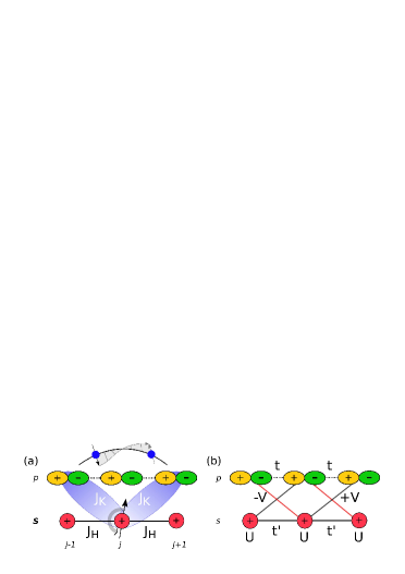
Figure 1: (a) Representation of the $p-$wave Kondo-Heisenberg model ($p$-KHM) in one dimension. The upper leg represents the conduction electron $p$-band, and the lower leg corresponds to a spin-1/2 Heisenberg chain. The Kondo exchange $J_{K}$ couples a spin $\mathbf{S}_{j}$ with the $p$-wave spin density in the conduction band [see Eq. (1)]. (b) Microscopic model effectively realizing the $p$-KHM at low energies, and allowing an experimental implementation in $p-$band optical lattices. At half-filling, the fermionic sites in the lower-leg behave as spins due to a strong on-site Hubbard repulsion $U$. The direct hopping across a given rung vanishes due to the different parities of the orbitals. The unusual $p-$wave Kondo interaction in 1(a) originates in second-order hopping processes in $V$, i.e., $J_{K}=8V^{2}/U$ (see Appendix A).

In order to gain further intuition into the effect of strong interactions, recently Alexandrov and Coleman (Alexandrov and Coleman, 2014) proposed an analytically tractable model for a one-dimensional (1D) TKI, i.e., the “$p$-wave” Kondo-Heisenberg model ($p$-KHM), consisting of a chain of spin-1/2 magnetic impurities interacting with a half-filled one-dimensional electron gas through a Kondo exchange [see Fig. 1(a)]. The peculiarity of this model, which makes it crucially different from other one-dimensional Kondo lattice models studied previously (Zachar et al., 1996; Sikkema et al., 1997; Zachar and Tsvelik, 2001; Tsunetsugu et al., 1992; Shibata et al., 1996, 1997; Tsunetsugu et al., 1997; Shibata and Ueda, 1999; Zachar, 2001; Berg et al., 2010; Dobry et al., 2013; Cho et al., 2014), is that the Kondo exchange couples to the “$p$-wave” conduction-electron spin density, allowing for effective next-nearest neighbor hopping processes in the conduction band accompanied by a spin-flip [see Fig. 1(a)]. Using a standard mean-field description (Read and Newns, 1983; Coleman, 1987; Newns and Read, 1987), the above authors found a topologically non-trivial insulating groundstate (i.e., a class-D insulator (Altland and Zirnbauer, 1997; Kitaev, 2009; Ryu et al., 2010)) which hosts magnetic states at the open ends of the chain. Soon after, two of us studied this system using the Abelian bosonization approach combined with a perturbative renormalization group analysis, revealing an unexpected connection to the Haldane phase at low temperatures (Lobos et al., 2015). The Haldane phase is a paradigmatic example of a strongly interacting topological system, with unique features such as topologically protected spin-1/2 end-states, non-vanishing string order parameter, and the breaking of a discrete $Z{}_{2}\times Z_{2}$ hidden symmetry in the groundstate (Affleck et al., 1987, 1989; Kennedy and Tasaki, 1992). The striking results in Ref. (Lobos et al., 2015) indicate that 1D TKI systems might be much more complex and richer than expected with the naïve mean-field approach, and suggest that they must be reconsidered from the more general perspective of interacting symmetry-protected topological phases (Pollmann et al., 2012; Wang and Senthil, 2014).

In this Letter we study the groundstate properties of the finite-length $p$-KHM in one dimension using the Density Matrix Renormalization Group (DMRG) (White, 1992, 1993). Our results indicate that the system is a Haldane insulator with protected spin-1/2 end-states and finite string order parameter, therefore supporting the predictions of Ref. (Lobos et al., 2015). We also propose that this exotic model could be realized in $p-$band optical lattices loaded with ultracold Fermi gases, which would allow for controlled experimental studies of TKIs in the lab.

Model. The Hamiltonian of the $p$-KHM is $H=H_{1}+H_{2}+H_{K}$ (Alexandrov and Coleman, 2014; Lobos et al., 2015), where the conduction band is represented by a $L$-site tight-binding chain $H_{1}=-t\sum_{j=1,\sigma}^{L-1}\left(p_{j,\sigma}^{\dagger}p_{j+1,\sigma}+\mbox{H.c.}\right)$ with $p_{j,\sigma}^{\dagger}$ the creation operator of an electron with spin $\sigma$ at site $j$ with spatial $p-$symmetry [upper leg in Fig. 1(a)]. The Hamiltonian $H_{2}=J_{H}\sum_{j=1}^{L-1}\mathbf{S}_{j}\cdot\mathbf{S}_{j+1}$ [bottom leg in Fig. 1(a)] corresponds to a spin 1/2 Heisenberg chain, and $H_{K}$ is the Kondo exchange coupling between $H_{1}$ and $H_{2}$ (Alexandrov and Coleman, 2014; Lobos et al., 2015)

$$H_{K} =J_{K}\sum_{j=1}^{L}\mathbf{S}_{j}\ .\ \boldsymbol{\pi}_{j},$$ (1)

with $J_{K}>0$. This Kondo interaction is unusual in that it couples the spin $\mathbf{S}_{j}$ in the Heisenberg chain to the “p-wave” spin density in the fermionic chain at site $j$, defined as $\boldsymbol{\pi}_{j}\equiv\sum_{\alpha,\beta}\bigl{(}\frac{p_{j+1,\alpha}^{\dagger}-p_{j-1,\alpha}^{\dagger}}{\sqrt{2}}\bigr{)}\bigl{(}\frac{\boldsymbol{\sigma}_{\alpha\beta}}{2}\bigr{)}\bigl{(}\frac{p_{j+1,\beta}-p_{j-1,\beta}}{\sqrt{2}}\bigr{)}$, where $p_{0,\sigma}=p_{L+1,\sigma}=0$ is implied, and where $\boldsymbol{\sigma}_{\alpha\beta}$ is the vector of Pauli matrices. Eq. (1) can be written as $H_{K}=H_{K}^{\left(1\right)}+H_{K}^{\left(2\right)}$, where $H_{K}^{\left(1\right)}=\frac{J_{K}}{2}\sum_{j}\mathbf{S}_{j}\ .\ \left(\mathbf{s}_{j-1}+\mathbf{s}_{j+1}\right)$ contains the coupling of a localized spin with the usual spin-density at site $j\pm 1$ in the conduction band (where $\mathbf{s}_{j}=\sum_{\alpha,\beta}p_{j,\alpha}^{\dagger}\bigl{(}\frac{\boldsymbol{\sigma}_{\alpha\beta}}{2}\bigr{)}p_{j,\beta}$), and $H_{K}^{\left(2\right)}=-\frac{J_{K}}{2}\sum_{j}\mathbf{S}_{j}\ .\ \left[\sum_{\alpha,\beta}p_{j+1,\alpha}^{\dagger}\bigl{(}\frac{\boldsymbol{\sigma}_{\alpha\beta}}{2}\bigr{)}p_{j-1,\beta}+\text{H.c.}\right]$ describes a different type of processes characterized by a non-local (i.e., next-nearest neighbor) hopping accompanied by a spin-flip.

We have studied the groundstate properties of $H$ by means of DMRG. In our implementation we have kept $m=800$ states, which allowed to achieve truncation errors in the density matrix of the order of $10^{-12}$. The DMRG method has been used previously to describe the standard 1D Kondo lattice model at half-filling (Tsunetsugu et al., 1992; Shibata et al., 1996, 1997; Tsunetsugu et al., 1997; Shibata and Ueda, 1999), where a topologically trivial, fully gapped groundstate was obtained. For the $p$-KHM, where a topological insulator groundstate was predicted (Alexandrov and Coleman, 2014; Lobos et al., 2015), there are no DMRG studies to the best of our knowledge. Intuitively, we expect that the charge and spin gaps in this model vanish in the limit $J_{K}\rightarrow 0$, as the Hamiltonians $H_{1}$ and $H_{2}$ are separately gapless in the thermodynamic limit. According to the bosonization analysis in the limit of small $J_{K}$, both gaps are favored when the velocities of the gapless spinon excitations described by $H_{1}$ and $H_{2}$ coincide (Lobos et al., 2015). Intuitively, the term $H_{K}$ becomes more effective to couple the spin degrees of freedom in $H_{1}$ and $H_{2}$ when they fluctuate coherently (i.e., same spinon velocities). The spinon velocity in the conduction band is equal to the tight-binding Fermi velocity $v_{1}=v_{F}=2t$, and in the Heisenberg chain is $v_{2}=\pi J_{H}/2$ (Luther and Peschel, 1975; Giamarchi, 2004), and therefore we conclude that the optimal situation in order to maximize the effect of $H_{K}$ corresponds to $J_{H}=4t/\pi\approx 1.27\ t$, which we choose in all our subsequent calculations. In what follows, we characterize the groundstate by analyzing the charge and spin gaps, the string order parameter, and spin profile along the chain.

Charge gap. Spin-flip scattering generated upon increasing $J_{K}$ induces gapped charge- and spin-excitations in the system at half filling (Alexandrov and Coleman, 2014; Lobos et al., 2015). Although these gaps are not direct evidence of the topological nature of the groundstate, their study is important to characterize the $p-$KHM insulating phase and to test the predictions of bosonization (Lobos et al., 2015). Using the hidden $SU\left(2\right)$ charge pseudo-spin symmetry of the model at half-filling, we can compute the charge gap of a $L-$supersite system as $\Delta_{\text{c}}\left(L\right)=E_{0}^{M^{z}=0}\left(N=L+2\right)-E_{0}^{M^{z}=0}\left(N=L\right)$ (Shibata et al., 1997; Shibata and Ueda, 1999). Here, a “supersite” $j$ refers to the combination of a spin $\mathbf{S}_{j}$ and the fermionic site in each rung. $M^{z}$ is the $z$-projection of the total spin in the system, computed as $M^{z}=\sum_{j=1}^{L}\langle T^{z}_{j}\rangle$, where $\mathbf{T}_{j}\equiv\mathbf{S}_{j}+\mathbf{s}_{j}$. Finally, $E_{0}^{M^{z}}\left(N\right)$ is the groundstate energy of a system with $N$ electrons in the conduction band, and projection $M^{z}$. While previous results on the standard 1D Kondo lattice predicted a linear dependence $\Delta_{\text{c}}\propto J_{K}$ (Zachar et al., 1996; Shibata and Ueda, 1999), here the presence of the Heisenberg coupling $J_{H}$ changes this behavior as it cancels the first order contribution (Lobos et al., 2015). The leading second-order contribution to $\Delta_{\text{c}}$ can be physically understood integrating out the “fast” spin fluctuations in the Heisenberg chain, which generate an effective repulsive four-fermion interaction $U^{\prime}\propto J_{K}^{2}\left\langle\mathbf{S}_{i}.\mathbf{S}_{j}\right\rangle_{H_{2}}$ in the conduction $p$-band. This effective interaction produce umklapp processes which open a Mott insulating gap at half-filling (Giamarchi, 2004). In Fig. 2 we show the charge gap as a function of $J_{K}$. The system presents important finite-size effects in the limit of small $J_{K}$, and we therefore analyze our results with the scaling law $\Delta_{\text{c}}\left(L\right)\approx\Delta_{\text{c}}\left(\infty\right)+\beta_{\text{c}}L^{-2}$ in the case of large $J_{K}$ ($J_{K}/t>0.3$) (Shibata et al., 1996; Shibata and Ueda, 1999), whereas in the regime of smaller $J_{K}/t<0.3$ the fits improve with the scaling law $\Delta_{\text{c}}\left(L\right)\approx\sqrt{\Delta^{2}_{\text{c}}\left(\infty\right)+\beta_{\text{c}}L^{-2}}$ (see inset in Fig. 2). This fitting procedure allows to extract $\Delta_{\text{c}}\left(\infty\right)$, the value of the charge gap in the thermodynamic limit, as a function of $J_{K}$ (see Fig. 2). The solid (red) line is a quadratic law $\Delta_{\text{c}}\left(\infty\right)=\alpha_{\text{c}}J_{K}^{2}$ which fits the data reasonably well at small $J_{K}$, confirming the dependence predicted by bosonization (Lobos et al., 2015).

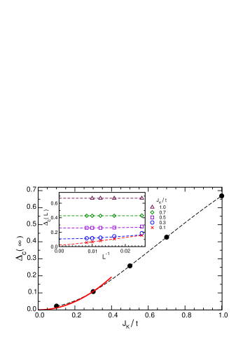
Figure 2: Charge gap $\Delta_{\text{c}}$ vs $J_{K}$. The circles are the values of the gap in the thermodynamical limit $\Delta_{\text{c}}\left(\infty\right)$, obtained after finite-size scaling (see inset). The solid (red) line is a fit $\Delta_{\text{c}}\left(\infty\right)=\alpha_{\text{c}}J_{K}^{2}$, valid for small $J_{K}$, based on the bosonization analysis of Ref. (Lobos et al., 2015). The dashed lines are a guide to the eye. Inset: Finite-size scaling using the scaling laws $\Delta_{\text{c}}\left(L\right)\approx\Delta_{\text{c}}\left(\infty\right)+\beta_{\text{c}}L^{-2}$ for $J_{K}/t>0.3$ (Shibata et al., 1996; Shibata and Ueda, 1999), and $\Delta_{\text{c}}\left(L\right)\approx\sqrt{\Delta^{2}_{\text{c}}\left(\infty\right)+\beta_{\text{c}}L^{-2}}$ for $J_{K}/t<0.3$.

Spin gap and spin-1/2 end states. We now focus on the spin degrees of freedom, where the $p$-KHM has the most interesting properties. Intuitively, the physics of the problem can be simply understood: the antiferromagnetic Kondo exchange along the diagonal rungs effectively forces the spins to align ferromagnetically across the rungs, even in the absence of a direct coupling (Lobos et al., 2015). This situation favors the formation of a local triplet in each supersite, and the system mimics the properties of the spin-1 Heisenberg chain (White and Huse, 1993) or the ferromagnetic Kondo lattice model (Tsunetsugu et al., 1992; Garcia et al., 2004), which are examples of systems realizing an insulating Haldane groundstate. A hallmark of this phase is the presence of two topologically protected spin-1/2 magnetic states at the ends of the chain (i.e., $\left|\uparrow\right\rangle_{L}\otimes\left|\uparrow\right\rangle_{R}$, $\left|\uparrow\right\rangle_{L}\otimes\left|\downarrow\right\rangle_{R}$, $\left|\downarrow\right\rangle_{L}\otimes\left|\uparrow\right\rangle_{R}$, and $\left|\downarrow\right\rangle_{L}\otimes\left|\downarrow\right\rangle_{R}$ ), which arrange into degenerate triplet and singlet linear combinations. As a result, the first spin-excitation gap $\Delta_{\text{s}}^{\left(1,0\right)}\left(L\right)\equiv E_{0}^{M^{z}=1}\left(N=L\right)-E_{0}^{M^{z}=0}\left(N=L\right)$, tends to zero for $L\rightarrow\infty$. For a finite-$L$ chain, however, the overlap of the end-states wavefunctions removes this degeneracy exponentially as $\Delta_{\text{s}}^{\left(1,0\right)}\left(L\right)\propto e^{-L/\xi}$, where $\xi\propto J_{K}^{-1}$ is the localization length for the magnetic end-states, and the groundstate for $N$ even (odd) corresponds to the singlet $S=0$ (triplet $S=1$) (White, 1993). In our case, at small $J_{K}$ the localization length $\xi$ becomes of the order of the system size ($\xi\sim L$), and it was not possible to obtain a conclusive scaling behavior for $\Delta_{\text{s}}^{\left(1,0\right)}$, even for the largest systems we have simulated ($L=120$). On the other hand, the gap $\Delta_{\text{s}}^{\left(2,0\right)}$ (same definition as above changing $M^{z}=1\rightarrow M^{z}=2$) can be identified with the Haldane gap of the system, and physically involves spin excitations which live in the bulk (see Fig. 3). In this case, the scaling analysis is simpler as it is free from edge effects, and we have used the scaling law $\Delta_{\text{s}}\left(L\right)\approx\sqrt{\Delta^{2}_{\text{s}}\left(\infty\right)+\beta_{\text{s}}L^{-2}}$ for all values of $J_{K}$ (see bottom inset in Fig. 3). The values of $\Delta_{\text{s}}\left(\infty\right)$ are shown in Fig. 3. In contrast to the case of the charge gap, here the analytic dependence of $\Delta_{\text{s}}\left(\infty\right)$ on the parameter $J_{K}$ is technically more challenging to obtain within the bosonization formalism, and is beyond the scope of this work. Nevertheless, our numerical results yield a power-law dependence $\Delta_{\text{s}}\left(\infty\right)\propto J_{K}^{\nu}$, with exponent $\nu\cong 2$.

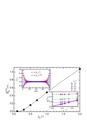
Figure 3: Spin gap $\Delta_{\text{s}}^{\left(2,0\right)}$ (physically corresponding to the Haldane gap in the system), as a function of $J_{K}$. The extrapolated spin gap $\Delta_{\text{s}}^{\left(2,0\right)}\left(\infty\right)$ is obtained after a finite-size scaling analysis (see bottom inset). The dashed lines are a guide to the eye. Top inset: Spatial profile of $\langle T^{z}_{j}\rangle=\langle\psi_{g}^{M^{z}=1}|T_{j}^{z}|\psi_{g}^{M^{z}=1}\rangle$, i.e., the $z$ component of the spin in the supersite $j$, computed with the groundstate of the subspace with total $M^{z}=1$ for $L=80$. The presence of the topologically protected spin-1/2 states at the ends of the chain is clearly seen. Bottom inset: Finite-size scaling using the scaling law $\Delta_{\text{s}}\left(L\right)\approx\sqrt{\Delta^{2}_{\text{s}}\left(\infty\right)+\beta_{\text{s}}L^{-2}}$.

We next investigate the presence of topologically protected spin-1/2 end-states which, as mentioned before, is a crucial feature of the open Haldane chain. In the upper inset of Fig. 3 we show a spatial profile of the $z-$projection of $\mathbf{T}_{j}$, i.e., $\left\langle T_{j}^{z}\right\rangle=\left\langle\psi_{g}^{M^{z}=1}\right|T_{j}^{z}\left|\psi_{g}^{M^{Z}=1}\right\rangle$, where $\left|\psi_{g}^{M^{z}=1}\right\rangle$ is the groundstate with total spin $M^{z}=1$, for $J_{K}/t=1$ and $J_{K}/t=2$. For these large values of $J_{K}$ (which are beyond the validity of the bosonization analysis (Lobos et al., 2015)) the end-states are clearly visible and show a small localization length $\xi$, a fact that prevents them from overlapping, producing negligible finite-size effects. Since we are working in the subspace $M^{z}=1$, and since the spin profile is symmetric under space inversion, we conclude that the spin accumulation at each end is 1/2, corresponding to the configuration where the topological spin-1/2 end-states is $\left|\psi_{g}^{M^{z}=1}\right\rangle\propto\left|\uparrow\right\rangle_{L}\otimes\left|\uparrow\right\rangle_{R}$ (Affleck et al., 1987, 1989).

String order parameter. The most fundamental signature of the Haldane phase is, however, the emergence of a finite string order parameter (den Nijs, 1992), a quantity deeply connected to a broken hidden $Z_{2}\times Z_{2}$ symmetry (Kennedy and Tasaki, 1992). This quantity is a smoking-gun for the presence of the Haldane phase, and therefore is the most important for our present purposes. Using the above definition of $\mathbf{T}_{j}$, the string order parameter is defined as $\mathcal{O}_{\text{string}}^{\alpha}\left(l-m\right)\equiv-\left\langle T_{l}^{\alpha}e^{i\pi\sum_{l<j<m}T_{j}^{\alpha}}T_{m}^{\alpha}\right\rangle$. Due to the $SU\left(2\right)$ spin-symmetry of the model, it is enough to calculate the computationally simpler component $\alpha=z$. We have computed $\mathcal{O}_{\text{string}}^{z}\left(l-m\right)$ taking the sites $l$ and $m$ symmetrically about the center of the system in order to minimize the effect of the edges. Note in the inset of Fig. 4 that $\mathcal{O}_{\text{string}}^{z}\left(d\right)$ converges rapidly as a function of the distance $d=\left|l-m\right|$ to the 1D-bulk value $\mathcal{O}_{\text{string}}^{z,\text{bulk}}$. In the main Fig. 4 we show $\mathcal{O}_{\text{string}}^{z,\text{bulk}}$ vs $J_{K}$, which remains finite throughout the whole studied regime. This indicates the presence of a Haldane-insulating phase even beyond the regime of small $J_{K}$ where the bosonization analysis in Ref. (Lobos et al., 2015) is valid. This result, together with the confirmation of the presence of spin-1/2 end states, are the most important results of this paper, as they provide conclusive evidence that the $p$-KHM realizes a Haldane insulating phase.

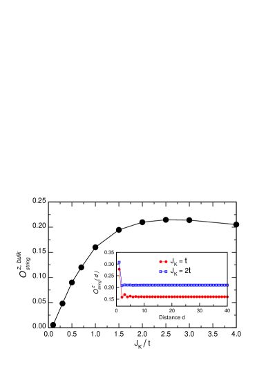
Figure 4: String order parameter $\mathcal{O}_{\text{string}}^{z,\text{bulk}}$ vs $J_{K}$. Throughout the whole studied regime, $\mathcal{O}_{\text{string}}^{z,\text{bulk}}$ remains finite, indicating the presence of a Haldane-insulating phase. Inset: Spatial dependence of $\mathcal{O}_{\text{string}}^{z}\left(d\right)$ vs the distance $d=\left|l-m\right|$, where $l$ and $m$ have been taken symmetrically about the center of the chain.

Realization in experimental systems. Recent experimental (Wirth et al., 2011; Soltan-Panahi et al., 2012; Lewenstein and Liu, 2015) and theoretical (Li et al., 2013; Liu et al., 2015) works on optical lattices with higher orbital $p-$bands suggest that the $p$-KHM could be realized in the laboratory. More specifically, the tight-binding Hamiltonian $H_{1}$ could be simulated populating the first excited energy level with $p-$symmetry at each site in a 1D optical lattice (see upper leg in Fig. 1(b)). The Heisenberg chain $H_{2}$ could be simulated with a half-filled Hubbard model in the Mott insulating phase (Schneider et al., 2008; Jördens et al., 2008), i.e., $H_{\text{Hubbard}}=-t^{\prime}\sum_{\left\langle ij\right\rangle,\sigma}^{N}\left(s_{i,\sigma}^{\dagger}s_{j,\sigma}+\mathrm{H.c.}\right)+U\sum_{i}^{N}\left(n_{i,\uparrow}^{\left(s\right)}-\frac{1}{2}\right)\left(n_{i,\downarrow}^{\left(s\right)}-\frac{1}{2}\right)$ in the limit $U\gg t^{\prime}$ (see lower leg in Fig. 1(b)), where $U$ is the on-site Coulomb interaction which could be tuned via a Feschbach resonance. Here $s_{j,\sigma}^{\dagger}$ is a creation operator of a fermion with spin $\sigma$ at the $s-$orbital site $j$, and $n_{j,\sigma}^{\left(s\right)}=s_{j,\sigma}^{\dagger}s_{j,\sigma}$ the fermion occupation. The unusual Kondo exchange $H_{K}$ would naturally arise in this situation if a microscopic single-particle hopping between $H_{1}$ and $H_{\text{Hubbard}}$ is allowed [see Fig. 1(b)]. Due to the different parities of the orbitals involved, the matrix element connecting the sites on the same rung (i.e., along the vertical direction) vanishes. The leading contribution therefore corresponds to the matrix element $V$ coupling $s$ and $p$ orbitals along a diagonal rung, i.e., $H_{\text{s-p}}=V\sum_{j,\sigma}s_{j,\sigma}^{\dagger}\left(p_{j+1,\sigma}-p_{j-1,\sigma}\right)+\text{H.c.}$, where the crucial sign inside the parentheses is a direct consequence of the $p-$wave nature of the conduction band states. The equivalence between the more “physical” Hamiltonian $H^{\prime}=H_{\text{Hubbard}}+H_{\text{s-p}}+H_{1}$ and the $p$-KHM can be rigorously shown by the means of a canonical (i.e., a generalized Schrieffer-Wolff) transformation $\mathcal{T}\equiv e^{i\mathcal{S}}$, where the operator $\mathcal{S}=\mathcal{S}\left(t^{\prime},V\right)$ must be chosen so as to eliminate first order contributions in $t^{\prime}$ and $V$. The procedure is standard and here we only outline the main steps (see Appendix A for details). Assuming the limit $t^{\prime},V\ll U$, we can expand the exponential in $\mathcal{T}$ and truncate the series at second order in $\left(t^{\prime}/U\right)$ and $\left(V/U\right)$, therefore obtaining $H=\mathcal{T}^{\dagger}H^{\prime}\mathcal{T}\approx H^{\prime}+i\left[\mathcal{S},H^{\prime}\right]+\frac{i^{2}}{2!}\left[\mathcal{S},\left[\mathcal{S},H^{\prime}\right]\right]$. We choose the transformation to be $\mathcal{S}=-i\left[\left(H_{t^{\prime}}^{+}-H_{t^{\prime}}^{-}\right)+2\left(H_{\text{s-p}}^{+}-H_{\text{s-p}}^{-}\right)\right]/U^{\prime}$, with $H_{t^{\prime}}^{+}=-t^{\prime}\sum_{\left\langle ij\right\rangle,\sigma}^{N}n_{i,\bar{\sigma}}^{\left(s\right)}s_{i,\sigma}^{\dagger}s_{j,\sigma}\left(1-n_{j,\bar{\sigma}}^{\left(s\right)}\right)$ and $H_{\text{s-p}}^{+}=V\sum_{i,\sigma}\left[n_{i,\bar{\sigma}}^{\left(s\right)}s_{i,\sigma}^{\dagger}\left(p_{i+1,\sigma}-p_{i-1,\sigma}\right)\right.$$\left.s_{i,\sigma}\left(1-n_{i,\bar{\sigma}}^{\left(s\right)}\right)\right]$, (with the notation $\left\langle ij\right\rangle$ indicating that $i$ and $j$ are nearest-neighbor sites), and where $H_{t^{\prime}}^{-}=\left(H_{t^{\prime}}^{+}\right)^{\dagger}$ and $H_{\text{s-p}}^{-}=\left(H_{\text{s-p}}^{+}\right)^{\dagger}$. It is easy to check that the first order contributions cancel, and therefore $H_{2}=-\frac{1}{U}\mathcal{P}\left(H_{t}^{-}H_{t}^{+}\right)\mathcal{P}$ and $H_{K}=-\frac{2}{U}\mathcal{P}\left(H_{\text{s-p}}^{-}H_{\text{s-p}}^{+}\right)\mathcal{P}$, where $\mathcal{P}$ is the projector onto the lowest subspace of $H_{\text{Hubbard}}$ (see Appendix A). The connection between both models is completed identifying the parameters as $J_{H}\equiv 4t^{\prime 2}/U$ and $J_{K}\equiv 8V^{2}/U$.

Note that this proposal is different from other theoretical proposals to simulate the standard Kondo lattice model in 1D optical lattices (Foss-Feig et al., 2010a, b).

Conclusions. We have studied the $p$-KHM, a theoretical “toy-model” introduced to describe a one-dimensional topological Kondo insulator, by the means of DMRG, and have calculated various quantities characterizing the properties of the groundstate at half-filling. We have shown strong numerical evidence (based on the analysis of the charge and spin gaps, the spin profile, and the string order parameter) that the $p$-KHM realizes a Haldane insulating phase at low temperatures, as predicted in Ref. (Lobos et al., 2015). Our results indicate that the topological properties of this model fall beyond the scope of the non-interacting topological classification (Altland and Zirnbauer, 1997; Kitaev, 2009; Ryu et al., 2010), which is unable to reveal the true topological structure of the groundstate. Finally, we have proposed that the unusual $p-$wave nature of the Kondo interaction could be physically realized in experiments with ultracold Fermi gases loaded in $p-$band optical lattices.

The authors acknowledge support from CONICET-PIP 00389CO.

Appendix A Derivation of the $p$-KHM by a Canonical Transformation

In this Appendix we provide a derivation of the $p$-KHM Hamiltonian $H$ in the main text by the means of a canonical transformation. To that end, we start from the microscopic Hamiltonian $H^{\prime}$, consisting of a fermionic Hubbard ladder with $s$ and $p$ orbitals along the legs, and depicted in Figure 1(b) in the main text:

$$H^{\prime}= H_{\text{Hubbard}}+H_{\text{s-p}}+H_{1},$$ (2)

$$H_{\text{Hubbard}}= -t^{\prime}\sum_{j,\sigma}^{L-1}\left(s_{j,\sigma}^{\dagger}s_{j+1,\sigma}+\mathrm{H.c.}\right)$$ (3)

$$+U\sum_{j=1}^{L}\left(n_{j,\uparrow}^{\left(s\right)}-\frac{1}{2}\right)\left(n_{j,\downarrow}^{\left(s\right)}-\frac{1}{2}\right),$$ (4)

$$H_{1}= -t\sum_{j=1,\sigma}^{L-1}\left(p_{j,\sigma}^{\dagger}p_{j+1,\sigma}+\mbox{H.c.}\right)$$ (5)

$$H_{\text{s-p}}= V\sum_{j,\sigma}s_{j,\sigma}^{\dagger}\left(p_{j+1,\sigma}-p_{j-1,\sigma}\right)+\text{H.c.},$$ (6)

Note that the system has electron-hole symmetry. Here, $s_{j,\sigma}^{\dagger}$ creates a fermion with spin projection $\sigma$ at site $j$ in the Hubbard leg and $n_{j\sigma}^{\left(s\right)}\equiv s_{j,\sigma}^{\dagger}s_{j,\sigma}$ is the corresponding fermion-number operator. The operator $p_{j,\sigma}^{\dagger}$ creates a fermion with spin $\sigma$ at site $j$ in the $p-$orbital conduction band, represented by a simple tight-binding model $H_{1}$. The term $H_{\text{s-p}}$ couples the two fermionic legs, and due to the symmetry properties of the $s-$ and $p-$orbitals, the direct hopping across the rungs is zero. Therefore, the most important hopping process occurs between a fermion $s_{j,\sigma}$ and the linear superposition with $p-$wave symmetry $\propto\left(p_{j+1,\sigma}-p_{j-1,\sigma}\right)$ in the conduction band.

The idea is to derive an effective low-energy model in the limit $U\gg\left\{t^{\prime},V\right\}$. To that end, we split the Hamiltonian $H^{\prime}$ into

$$H^{\prime} =H_{t^{\prime}}+H_{\text{s-p}}+H_{U}+H_{1},$$ (7)

where

$$H_{t^{\prime}} =-t^{\prime}\sum_{\left\langle ij\right\rangle,\sigma}^{L}\left(s_{i,\sigma}^{\dagger}s_{j,\sigma}+\mathrm{H.c.}\right),$$ (8)

$$H_{U} =U\sum_{j}^{L}\left(n_{j,\uparrow}-\frac{1}{2}\right)\left(n_{j,\downarrow}-\frac{1}{2}\right).$$ (9)

The first two terms in (7) will be considered as perturbations to $H_{U}$, in the regime $\left\{t^{\prime},V\right\}\ll U$.

We now start from the atomic limit in the Hubbard leg, i.e., $t^{\prime}=V=0$, and identify the atomic singly-occupied states $\left|\sigma_{j}\right\rangle=s_{j,\sigma}^{\dagger}\left|0\right\rangle$ ($\sigma=\uparrow,\downarrow$) as forming the lowest-energy subspace at site $j$, while the $\left|0_{j}\right\rangle$ (empty) and $\left|d_{j}\right\rangle=s_{j,\uparrow}^{\dagger}s_{j,\downarrow}^{\dagger}\left|0\right\rangle$ (doubly-occupied) form the excited subspace. We now introduce projectors onto each of the 4 atomic states:

$$\mathcal{P}_{j,0} =\left(1-n_{j,\uparrow}^{\left(s\right)}\right)\left(1-n_{j,\downarrow}^{\left(s\right)}\right),$$ (10)

$$\mathcal{P}_{j,d} =n_{j,\uparrow}^{\left(s\right)}n_{j,\downarrow}^{\left(s\right)},$$ (11)

$$\mathcal{P}_{j,\uparrow} =n_{j,\uparrow}^{\left(s\right)}\left(1-n_{j,\downarrow}^{\left(s\right)}\right),$$ (12)

$$\mathcal{P}_{j,\downarrow} =n_{j,\downarrow}^{\left(s\right)}\left(1-n_{j,\uparrow}^{\left(s\right)}\right).$$ (13)

Note that while all projectors commute with $H_{U}$, the kinetic terms $H_{t^{\prime}}$ and $H_{\text{s-p}}$ cause transitions among subspaces. Using that $\mathbf{1}_{j}=\sum_{\alpha}\mathcal{P}_{j,\alpha}$, we can write the kinetic terms as $H_{t^{\prime}}=\left(\sum_{i,\alpha}\mathcal{P}_{i,\alpha}\right)H_{t^{\prime}}\left(\sum_{j,\beta}\mathcal{P}_{j,\beta}\right)=H_{t^{\prime}}^{+}+H_{t^{\prime}}^{-}+H_{t^{\prime}}^{0},$ and $H_{\text{s-p}}=\left(\sum_{i,\alpha}\mathcal{P}_{i,\alpha}\right)H_{\text{s-p}}\left(\sum_{j,\beta}\mathcal{P}_{j,\beta}\right)=H_{\text{s-p}}^{+}+H_{\text{s-p}}^{-}+H_{\text{s-p}}^{0},$ where

$$H_{t^{\prime}}^{+} =-t^{\prime}\sum_{\left\langle ij\right\rangle,\sigma}^{N}\left[n_{i,\bar{\sigma}}^{\left(s\right)}s_{i,\sigma}^{\dagger}s_{j,\sigma}\left(1-n_{j,\bar{\sigma}}^{\left(s\right)}\right)+n_{j,\bar{\sigma}}^{\left(s\right)}s_{j,\sigma}^{\dagger}s_{i,\sigma}\left(1-n_{i,\bar{\sigma}}^{\left(s\right)}\right)\right],$$ (14)

$$H_{t^{\prime}}^{-} =-t^{\prime}\sum_{\left\langle ij\right\rangle,\sigma}^{N}\left[\left(1-n_{j,\bar{\sigma}}^{\left(s\right)}\right)s_{j,\sigma}^{\dagger}s_{i,\sigma}n_{i,\bar{\sigma}}^{\left(s\right)}+\left(1-n_{i,\bar{\sigma}}^{\left(s\right)}\right)s_{i,\sigma}^{\dagger}s_{j,\sigma}n_{j,\bar{\sigma}}^{\left(s\right)}\right],$$ (15)

$$H_{\text{s-p}}^{+} =V\sum_{i,\sigma}\left[n_{i,\bar{\sigma}}^{\left(s\right)}s_{i,\sigma}^{\dagger}\left(p_{i+1,\sigma}-p_{i-1,\sigma}\right)+\left(p_{i+1,\sigma}^{\dagger}-p_{i-1,\sigma}^{\dagger}\right)s_{i,\sigma}\left(1-n_{i,\bar{\sigma}}^{\left(s\right)}\right)\right],$$ (16)

$$H_{\text{s-p}}^{-} =V\sum_{i,\sigma}\left[\left(p_{i+1,\sigma}^{\dagger}-p_{i-1,\sigma}^{\dagger}\right)s_{i,\sigma}n_{i,\bar{\sigma}}^{\left(s\right)}+\left(1-n_{i,\bar{\sigma}}^{\left(s\right)}\right)s_{i,\sigma}^{\dagger}\left(p_{i+1,\sigma}-p_{i-1,\sigma}\right)\right].$$ (17)

Physically, the term with supraindex “$+$” produce transitions from the lowest subspace to the excited subspace, while those with “$-$” restore excited states to the lowest subspace. On the other hand, the terms labelled with “$0$” do not change the subspace, and since we assume a half-filled conduction band, they will identically vanish and it is not necessary to write them explicitly here. We now note the following important relations

$$H_{t^{\prime}}^{-} =\left(H_{t^{\prime}}^{+}\right)^{\dagger},$$ (18)

$$H_{\text{s-p}}^{-} =\left(H_{\text{s-p}}^{+}\right)^{\dagger},$$ (19)

which will be useful in what follows.

We now introduce a canonical transformation in Eq. (2), such that in the transformed representation we simultaneously get rid of the terms at first order in $t^{\prime}$ and $V$:

$$H =e^{i\mathcal{S}}H^{\prime}e^{-i\mathcal{S}}.$$ (20)

$$=H^{\prime}+i\left[\mathcal{S},H^{\prime}\right]+\frac{i^{2}}{2!}\left[\mathcal{S},\left[\mathcal{S},H^{\prime}\right]\right]+\dots$$ (21)

We want to choose $\mathcal{S}$ in such a way that $H$ does not connect different Hubbard subbands. Note that this cannot be achieved at infinite order in the expansion in powers of $\mathcal{S}$ in Eq. (21), but we will be content if we can eliminate the contributions at order $\mathcal{O}\left(t^{\prime}\right)$ and $\mathcal{O}\left(V\right)$ that mix the subbands. We now write the expansion in Eq. (21) in the more suggestive form

$$H =H_{t^{\prime}}^{+}+H_{t^{\prime}}^{-}+H_{\text{s-p}}^{+}+H_{\text{s-p}}^{-}+i\left[\mathcal{S},H_{U}\right]$$ (22)

$$+H_{1}+H_{U}+i\left[\mathcal{S},H_{t^{\prime}}^{+}+H_{t^{\prime}}^{-}\right]+i\left[\mathcal{S},H_{\text{s-p}}^{+}+H_{\text{s-p}}^{-}\right]$$ (23)

$$+\frac{i^{2}}{2!}\left[\mathcal{S},\left[\mathcal{S},H_{U}\right]\right]+\text{(other less important terms})$$ (24)

We will require that the first line (22) in the above equation vanishes. It is then clear that $\mathcal{S}$ must be $\mathcal{O}\left(t^{\prime}/U\right)\sim\mathcal{O}\left(V/U\right)$. Using the following results

$$\left[n_{i,\bar{\sigma}}^{\left(s\right)}s_{i,\sigma}^{\dagger}s_{j,\sigma}\left(1-n_{j,\bar{\sigma}}^{\left(s\right)}\right),\left(n_{i,\sigma}^{\left(s\right)}-\frac{1}{2}\right)\left(n_{i,\bar{\sigma}}^{\left(s\right)}-\frac{1}{2}\right)\right] =\left[n_{i,\bar{\sigma}}^{\left(s\right)}s_{i,\sigma}^{\dagger}s_{j,\sigma}\left(1-n_{j,\bar{\sigma}}^{\left(s\right)}\right),\left(n_{j,\sigma}^{\left(s\right)}-\frac{1}{2}\right)\left(n_{j,\bar{\sigma}}^{\left(s\right)}-\frac{1}{2}\right)\right]$$ (25)

$$=-\frac{1}{2}n_{i,\bar{\sigma}}^{\left(s\right)}s_{i,\sigma}^{\dagger}s_{j,\sigma}\left(1-n_{j,\bar{\sigma}}^{\left(s\right)}\right),$$ (26)

$$\left[n_{i,\bar{\sigma}}^{\left(s\right)}s_{i,\sigma}^{\dagger}\left(p_{i+1,\sigma}-p_{i-1,\sigma}\right),\left(n_{i,\sigma}^{\left(s\right)}-\frac{1}{2}\right)\left(n_{i,\bar{\sigma}}^{\left(s\right)}-\frac{1}{2}\right)\right] =-\frac{1}{2}n_{i,\bar{\sigma}}^{\left(s\right)}s_{i,\sigma}^{\dagger}\left(p_{i+1,\sigma}-p_{i-1,\sigma}\right),$$ (27)

$$\left[\left(p_{i+1,\sigma}^{\dagger}-p_{i-1,\sigma}^{\dagger}\right)s_{i,\sigma}\left(1-n_{i,\bar{\sigma}}^{\left(s\right)}\right),\left(n_{i,\sigma}^{\left(s\right)}-\frac{1}{2}\right)\left(n_{i,\bar{\sigma}}^{\left(s\right)}-\frac{1}{2}\right)\right] =-\frac{1}{2}\left(p_{i+1,\sigma}^{\dagger}-p_{i-1,\sigma}^{\dagger}\right)s_{i,\sigma}\left(1-n_{i,\bar{\sigma}}^{\left(s\right)}\right),$$ (28)

it is easy to check that

$$\left[H_{t^{\prime}}^{\pm},H_{U}\right] =\mp UH_{t^{\prime}}^{\pm},$$ (29)

$$\left[H_{\text{s-p}}^{\pm},H_{U}\right] =\mp\frac{U}{2}H_{\text{s-p}}^{\pm}.$$ (30)

Then, it follows that the choice

$$\mathcal{S} =-\frac{i}{U}\left(H_{t^{\prime}}^{+}-H_{t^{\prime}}^{-}\right)-\frac{2i}{U}\left(H_{\text{s-p}}^{+}-H_{\text{s-p}}^{-}\right),$$ (31)

exactly cancels line (22).

The relevant part of the Hamiltonian at low energies is then obtained projecting $H$ onto the lowest Hubbard subband. This is formally done applying the projector $\mathcal{P}=\sum_{i}\left(\mathcal{P}_{i,\uparrow}+\mathcal{P}_{i,\downarrow}\right)$, which eliminates certain terms in Eqs. (23) and (24). The resulting effective Hamiltonian at lowest order in $t/U$ and $V/U$ is therefore

$$H =H_{1}+\mathcal{P}\left\{H_{U}+i\left[\mathcal{S},H_{t^{\prime}}^{+}+H_{t^{\prime}}^{-}\right]+i\left[\mathcal{S},H_{\text{s-p}}^{+}+H_{\text{s-p}}^{-}\right]+\frac{i^{2}}{2!}\left[\mathcal{S},\left[\mathcal{S},H_{U}\right]\right]\right\}\mathcal{P},$$

$$=H_{1}+H_{U}-\frac{1}{U}\mathcal{P}\left(H_{t^{\prime}}^{-}H_{t^{\prime}}^{+}\right)\mathcal{P}-\frac{2}{U}\mathcal{P}\left(H_{\text{s-p}}^{-}H_{\text{s-p}}^{+}\right)\mathcal{P}.$$ (32)

We now replace the expressions for $H_{t^{\prime}}^{\pm}$ and $H_{\text{s-p}}^{\pm}$ [Eqs. (14)-(17)] into the above equation and obtain

$$\mathcal{P}\left(H_{t^{\prime}}^{-}H_{t^{\prime}}^{+}\right)\mathcal{P} =\left(t^{\prime}\right)^{2}\sum_{i,\sigma}^{N}\left[\mathcal{P}_{i,\bar{\sigma}}\mathcal{P}_{i+1,\sigma}+\mathcal{P}_{i,\sigma}\mathcal{P}_{i+1,\bar{\sigma}}-s_{i+1,\sigma}^{\dagger}s_{i+1,\bar{\sigma}}s_{i,\bar{\sigma}}^{\dagger}s_{i,\sigma}-s_{i+1,\bar{\sigma}}^{\dagger}s_{i+1,\sigma}s_{i,\sigma}^{\dagger}s_{i,\bar{\sigma}}\right]$$ (33)

$$\mathcal{P}\left(H_{\text{s-p}}^{-}H_{\text{s-p}}^{+}\right)\mathcal{P} =2V^{2}\sum_{i,\sigma}n_{i,\sigma}^{\left(s\right)}-V^{2}\sum_{i,\sigma}\left[\left(n_{i,\sigma}^{\left(s\right)}-n_{i,\bar{\sigma}}^{\left(s\right)}\right)\left(p_{i+1,\sigma}^{\dagger}-p_{i-1,\sigma}^{\dagger}\right)\left(p_{i+1,\sigma}-p_{i-1,\sigma}\right)\right.$$

$$\left.+s_{i,\bar{\sigma}}^{\dagger}s_{i,\sigma}\left(p_{i+1,\sigma}^{\dagger}-p_{i-1,\sigma}^{\dagger}\right)\left(p_{i+1,\bar{\sigma}}-p_{i-1,\bar{\sigma}}\right)+s_{i,\sigma}^{\dagger}s_{i,\bar{\sigma}}\left(p_{i+1,\bar{\sigma}}^{\dagger}-p_{i-1,\bar{\sigma}}^{\dagger}\right)\left(p_{i+1,\sigma}-p_{i-1,\sigma}\right)\right]$$ (34)

Using that $\mathcal{P}_{i,\uparrow}\mathcal{P}_{i+1,\downarrow}+\mathcal{P}_{i,\downarrow}\mathcal{P}_{i+1,\uparrow}=-2S_{i}^{z}S_{i+1}^{z}+n_{i}^{\left(s\right)}n_{i+1}^{\left(s\right)}/2$, and the Schwinger-fermion representation

$$S_{i}^{z} =\frac{n_{i,\uparrow}^{\left(s\right)}-n_{i,\downarrow}^{\left(s\right)}}{2},$$ (35)

$$S_{i}^{+} =s_{i,\uparrow}^{\dagger}s_{i,\downarrow},$$ (36)

$$S_{i}^{-} =s_{i,\downarrow}^{\dagger}s_{i,\uparrow},$$ (37)

is a faithful representation of a spin-1/2 operator, we can write the effective Hamiltonian as

$$H =H_{U}+H_{1}+\frac{4\left(t^{\prime}\right)^{2}}{U}\sum_{i}^{N}\left[S_{i}^{z}S_{i+1}^{z}+\frac{S_{i+1}^{+}S_{i}^{-}+S_{i+1}^{-}S_{i}^{+}}{2}-\frac{1}{4}\right]$$

$$+\frac{8V^{2}}{U}\sum_{i}S_{i}^{z}\frac{\left(p_{i+1,\uparrow}^{\dagger}-p_{i-1,\uparrow}^{\dagger}\right)\left(p_{i+1,\uparrow}-p_{i-1,\uparrow}\right)-\left(p_{i+1,\downarrow}^{\dagger}-p_{i-1,\downarrow}^{\dagger}\right)\left(p_{i+1,\downarrow}-p_{i-1,\downarrow}\right)}{2}$$

$$+\frac{8V^{2}}{U}\sum_{i}\left[\frac{S_{i}^{+}\left(p_{i+1,\downarrow}^{\dagger}-p_{i-1,\downarrow}^{\dagger}\right)\left(p_{i+1,\uparrow}-p_{i-1,\uparrow}\right)}{2}+\frac{S_{i}^{-}\left(p_{i+1,\uparrow}^{\dagger}-p_{i-1,\uparrow}^{\dagger}\right)\left(p_{i+1,\downarrow}-p_{i-1,\downarrow}\right)}{2}\right]$$ (38)

where we have neglected the constant $\frac{2V^{2}}{U}\sum_{i,\sigma}n_{i,\sigma}^{\left(s\right)}$. Defining the effective parameters

$$J_{H} \equiv\frac{4\left(t^{\prime}\right)^{2}}{U},$$ (39)

$$J_{K} \equiv\frac{8V^{2}}{U},$$ (40)

we note that this Hamiltonian corresponds to the $p$-KHM considered by Alexandrov and Coleman (Alexandrov and Coleman, 2014).

References

Dzero et al. (2010)
M. Dzero,
K. Sun,
V. Galitski, and
P. Coleman,
Phys. Rev. Lett. 104,
106408 (2010).
Dzero et al. (2012)
M. Dzero,
K. Sun,
P. Coleman, and
V. Galitski,
Phys. Rev. B 85,
045130 (2012).
Dzero et al. (2015)
M. Dzero,
J. Xia,
V. Galitski,
and
P. Coleman,
ArXiv e-prints (2015),
eprint 1506.05635.
Read and Newns (1983)
N. Read and
D. M. Newns,
J. Phys. C 16,
3273 (1983).
Coleman (1987)
P. Coleman,
Phys. Rev. B 35,
5072 (1987).
Newns and Read (1987)
D. M. Newns and
N. Read,
Adv.Phys. 36,
799 (1987).
Wolgast et al. (2013)
S. Wolgast,
C. Kurdak,
K. Sun,
J. W. Allen,
D.-J. Kim, and
Z. Fisk,
Phys. Rev. B 88,
180405 (2013).
Zhang et al. (2013)
X. Zhang,
N. P. Butch,
P. Syers,
S. Ziemak,
R. L. Greene,
and J. Paglione,
Phys. Rev. X 3,
011011 (2013).
Xu et al. (2014)
N. Xu et al.,
Nat. Commun. 5,
4566 (2014).
Kim et al. (2014)
D. J. Kim,
J. Xia, and
Z. Fisk,
Nat. Mater. 13,
466 (2014).
Alexandrov and
Coleman (2014)
V. Alexandrov and
P. Coleman,
Phys. Rev. B 90,
115147 (2014).
Zachar et al. (1996)
O. Zachar,
S. A. Kivelson,
and V. J. Emery,
Phys. Rev. Lett. 77,
1342 (1996).
Sikkema et al. (1997)
A. E. Sikkema,
I. Affleck, and
S. R. White,
Phys. Rev. Lett. 79,
929 (1997).
Zachar and Tsvelik (2001)
O. Zachar and
A. M. Tsvelik,
Phys. Rev. B 64,
033103 (2001),
cond-mat/9909296.
Tsunetsugu et al. (1992)
H. Tsunetsugu,
Y. Hatsugai,
K. Ueda, and
M. Sigrist,
Phys. Rev. B 46,
3175 (1992).
Shibata et al. (1996)
N. Shibata,
T. Nishino,
K. Ueda, and
C. Ishii,
Phys. Rev. B 53,
R8828 (1996).
Shibata et al. (1997)
N. Shibata,
A. Tsvelik, and
K. Ueda,
Phys. Rev. B 56,
330 (1997).
Tsunetsugu et al. (1997)
H. Tsunetsugu,
M. Sigrist, and
K. Ueda,
Rev. Mod. Phys. 69,
809 (1997).
Shibata and Ueda (1999)
N. Shibata and
K. Ueda, J.
Phys.: Condens. Matter 11, R1
(1999).
Zachar (2001)
O. Zachar,
Phys. Rev. B 63,
205104 (2001).
Berg et al. (2010)
E. Berg,
E. Fradkin, and
S. A. Kivelson,
Phys. Rev. Lett. 105,
146403 (2010).
Dobry et al. (2013)
A. Dobry,
A. Jaefari, and
E. Fradkin,
Phys. Rev. B 87,
245102 (2013).
Cho et al. (2014)
G. Y. Cho,
R. Soto-Garrido,
and
E. Fradkin,
ArXiv e-prints (2014),
eprint 1407.6358.
Altland and
Zirnbauer (1997)
A. Altland and
M. R. Zirnbauer,
Phys. Rev. B 55,
1142 (1997).
Kitaev (2009)
A. Kitaev, AIP
Conf. Proc. 1134, 22
(2009).
Ryu et al. (2010)
S. Ryu,
A. P. Schnyder,
A. Furusaki, and
A. W. W. Ludwig,
New Journal of Physics 12,
065010 (2010).
Lobos et al. (2015)
A. M. Lobos,
A. O. Dobry, and
V. Galitski,
Phys. Rev. X 5,
021017 (2015).
Affleck et al. (1987)
I. Affleck,
T. Kennedy,
E. H. Lieb, and
H. Tasaki,
Phys. Rev. Lett. 59,
799 (1987).
Affleck et al. (1989)
I. Affleck,
T. Kennedy,
E. H. Lieb, and
H. Tasaki,
Commun . Math. Phys. 115,
477 (1989).
Kennedy and Tasaki (1992)
T. Kennedy and
H. Tasaki,
Phys. Rev. B 45,
304 (1992).
Pollmann et al. (2012)
F. Pollmann,
E. Berg,
A. M. Turner,
and M. Oshikawa,
Phys. Rev. B 85,
075125 (2012).
Wang and Senthil (2014)
C. Wang and
T. Senthil,
Phys. Rev. B 89,
195124 (2014).
White (1992)
S. R. White,
Phys. Rev. Lett. 69,
2863 (1992).
White (1993)
S. R. White,
Phys. Rev. B 48,
10345 (1993).
Luther and Peschel (1975)
A. Luther and
I. Peschel,
Phys. Rev. B 12,
3908 (1975).
Giamarchi (2004)
T. Giamarchi,
Quantum Physics in One Dimension
(Oxford University Press, Oxford,
2004).
White and
Huse (1993)
S. R. White and
D. A. Huse,
Phys. Rev. B 48,
3844 (1993).
Garcia et al. (2004)
D. J. Garcia,
K. Hallberg,
B. Alascio, and
M. Avignon,
Phys. Rev. Lett. 93,
177204 (2004).
den Nijs (1992)
M. den Nijs,
Phys. Rev. B 46,
10386 (1992).
Wirth et al. (2011)
G. Wirth,
M. Ölschläger,
and
A. Hemmerich,
Nat. Phys. 7,
147 (2011).
Soltan-Panahi et al. (2012)
P. Soltan-Panahi,
D.-S. Lühmann,
J. Struck,
P. Windpassinger,
and
K. Sengstock,
Nat. Phys. 8,
71 (2012).
Lewenstein and Liu (2015)
M. Lewenstein and
W. V. Liu,
Nat. Phys. 7,
101 (2015).
Li et al. (2013)
X. Li,
E. Zhao, and
V. Liu,
Nature Communications 4,
1523 (2013).
Liu et al. (2015)
B. Liu,
X. Li,
R. G. Hulet,
and W. V. Liu,
ArXiv e-prints (2015),
eprint 1505.08164.
Schneider et al. (2008)
U. Schneider,
L. Hackermüller,
S. Will,
T. Best,
I. Bloch,
T. A. Costi,
R. W. Helmes,
D. Rasch, and
A. Rosch,
Science 322,
1520 (2008).
Jördens et al. (2008)
R. Jördens,
N. Strohmaier,
K. Günter,
H. Moritz, and
T. Esslinger,
Nature 455,
204 (2008).
Foss-Feig
et al. (2010a)
M. Foss-Feig,
M. Hermele, and
A. M. Rey,
Phys. Rev. A 81,
051603 (2010a).
Foss-Feig
et al. (2010b)
M. Foss-Feig,
M. Hermele,
V. Gurarie, and
A. M. Rey,
Phys. Rev. A 82,
053624 (2010b).