The sigma meson from lattice QCD with two-pion interpolating operators

Dean Howarth and Joel Giedt

Department of Physics, Applied Physics and Astronomy
Rensselaer Polytechnic Institute, 110 8th Street, Troy, NY 12180 USA

In this article we describe our studies of the sigma meson, ${f_{0}(500)}$, using two-pion correlation functions. We use lattice quantum chromodynamics in the quenched approximation with so-called clover fermions. By working at unphysical pion masses we are able to identify a would-be resonance with mass less than $2m_{\pi}$, and then extrapolate to the physical point. We include the most important annihilation diagram, which is “partially disconnnected” or “single annihilation.” Because this diagram is quite expensive to compute, we introduce a somewhat novel technique for the computation of all-to-all diagrams, based on momentum sources and a truncation in momentum space. In practice, we use only ${\bf p}=0$ modes, so the method reduces to wall sources. At the point where the mass of the pion takes its physical value, we find a resonance in the $0^{++}$ two-pion channel with a mass of approximately $609\pm 80$ MeV, consistent with the expected properties of the sigma meson, given the approximations we are making.

1 Motivation

Scalar resonances in quantum chromodynamics (QCD) have proven to be challenging objects to study in terms of experimental observation, computational studies, and theoretical explanation. The most elusive of these scalar states are arguably the ${f_{0}(500)}$ or $\sigma$ resonance, and the lightest scalar meson with nonzero strangeness, the $\kappa(900)$. As far as the $I=0$ state is concerned, many experiments over the years have found a broad enhancement in the two-pion spectrum, beginning at threshold and continuing to around 900 MeV: for instance a $\pi^{-}p\to\pi^{-}\pi^{+}n$ experiment at 17 GeV that ran at CERN 1970-1971 [1], $pp\to pp\pi^{0}\pi^{0}$ at 450 GeV by the GAMS NA12/2 collaboration also at CERN [2], $\pi^{-}p\to\pi^{0}\pi^{0}n$ at 18.3 GeV by the Brookhaven E852 experiment [3], and $J/\psi\to\omega\pi^{+}\pi^{-}$ by BES II [4]. If anything, the quality of the data has improved over time revealing that the enhancement takes on the shape of a very broad peak centered at around 500 MeV with a comparable width—though the shape may also have something to do with the channel in which the two-pion invariant mass was explored. Also over the years, there have been several lattice calculations of scalar correlation functions in the $I=0$ $J^{PC}=0^{++}$ channel, but many of them do not include annihilation diagrams that couple to the vacuum (see for instance Figs. 1(b) and 1(c) below) [5, 6, 7, 8, 9, 10, 11, 12, 13, 14, 15, 16]. Analysis of $0^{++}$ glueballs in full QCD [17] should also shed light on these states, due to mixing. The LHCb collaboration [18] report that the ${f_{0}(500)}$ is not a mesonic bound state according to their models, and present (model dependent) upper limits of the mixing of the ${f_{0}(500)}$ between $\bar{u}u+\bar{d}d$ and $\bar{s}s$ constituent quark states. There are several questions that remain open, e.g.,

• The width and mass of the resonance are comparable. While the shape does not agree with the two-pion continuum spectrum, it is possible that strong interaction effects between the two pions could produce such a spectrum, calling into question its identification as a true resonance in the classic sense of the word.

• Though the quantum numbers of the ${f_{0}(500)}$ are easy to discern, its partonic content is not known with any degree of confidence. One would certainly expect a large contribution from first generation quarks, and the possibility of contributions from the strange quark are certainly feasible. There is also the question of contributions from purely gluonic states, as yet seen only on the lattice. However, it is usually assumed that this contribution is small since the glueball in quenched lattice QCD has a mass around 1.6 GeV.

• The scattering phase of the two pseudoscalars in this channel ought to shift by $\pi$ radians if the intermediate state were a coherent and distinct quantum state that behaved like a Breit-Wigner resonance; it is possible that a more general two-meson bound state would give a smaller shift. Confusingly, the 1974 CERN-Munich measurements [19] of this phase shift give an intermediate value of only $\pi/2$ radians. A possible explanation was offered by Ishida et al. [20] whereby a “repulsive core” in the ${f_{0}(500)}$ induces a negative background phase to account for the “missing” phase shift of the channel. However, for a long time this lack of an adequate phase shift has cast doubt on the existence of the ${f_{0}(500)}$. Subsequent fits such as [21, 22] have seemingly alleviated this problem, apparently by avoiding the assumption of a Breit-Wigner type phase shift.

• There are also indirect uncertainties about the ${f_{0}(500)}$ in the context of its role in a scalar nonet [23, 24] and also a chiral scalar nonet [25]. The ${f_{0}(500)}$ can also play the role of a ‘Higgs boson’ in the context of lightest pseudoscalar mesons being the Nambu-Goldstone bosons of a (broken) chiral symmetry. This idea can be extended to “walking technicolor” models whereby the longitudinal components of the electroweak gauge bosons ($W^{\pm}$, $Z^{0}$) are described as composite particles known as techni-pions composed of techni-quarks. In fact, the Higgs boson has even been proposed as the pseudo-Nambu-Goldstone boson of scale invariance (see [26] for a review). So one wonders whether there is any connection between ${f_{0}(500)}$ and scale invariance in QCD.

Lattice QCD can shed light on some of these matters from a model independent, ab initio perspective. By identifying the ${f_{0}(500)}$ state on the lattice, we can measure its mass and other properties using well established techniques. A further, much more demanding study, is to use Lüscher’s method to measure the $I=0$, $L=0$ scattering phase shift $\delta_{0}^{0}$ of the $\pi^{+}\pi^{-}\to\pi^{+}\pi^{-}$ system, as has been done recently in a quite heroic effort [16]. This measurement has the benefit of not requiring a partial wave analysis with several intermediate states fit simultaneously, as is necessary in the experimental approach. In the calculation presented here, we show how the ground state energy of the $\pi^{+}\pi^{-}\to\pi^{+}\pi^{-}$ system at six different pion masses evolves with bare quark mass $m_{0}$ and that a linear extrapolation of these masses to physical scales indicates that the observed ground state is that of the ${f_{0}(500)}$. Given that the principal decay of the ${\sigma}$ is probably to $\pi\pi$ states, it seems that there should be a strong coupling to the interpolating operators that we use. It is also suggested by the tetraquark proposal for this state [27, 28]. Our work is quite similar to [8], including working at heavy pion masses where the would-be resonance lies below $2m_{\pi}$. Here, however we include the partially disconnected (single annihilation) diagrams, Figs. 1(c) and 1(d).

2 The four-point pseudoscalar correlation function

In order to study a $0^{++}$ scalar state such as the ${f_{0}(500)}$ we must create a state on the lattice with the same quantum numbers. One such state is $\pi^{+}\pi^{-}$ which we can create by inserting pseudoscalar creation operators $P^{+\dagger}$ and $P^{-\dagger}$ at at $({\bf 0},0)$ and (x,0) respectively. We then destroy the pseudoscalars at (y,t) and (z,t), leading to the correlation function

$$C(t)=\langle\Omega|T\{P^{-}({\bf z},t)P^{+}({\bf y},t)P^{-\dagger}({\bf x},0)P^{+\dagger}({\bf 0},0)\}|\Omega\rangle,$$ (1)

where in terms of the quark fields

$$P^{+\dagger}({\bf x},t) =\bar{u}({\bf x},t)\gamma_{5}d({\bf x},t),$$

$$P^{-\dagger}({\bf x},t) =\bar{d}({\bf x},t)\gamma_{5}u({\bf x},t).$$ (2)

For notational convenience we work with the understanding that the points $y$ and $z$ are located at timeslice $t\geq 0$, and $x$ and 0 are located at $t_{0}=0$. After performing the relevant Wick contractions there are four distinct propagator diagrams, illustrated in Fig. 1. We subtract from each relevant correlation function the (truly) disconnected pieces to leave only the truly connected part and average over gauge field configurations.

Since we are calculating $\pi^{+}\pi^{-}\to\pi^{+}\pi^{-}$ with zero momentum pions, both $I=0$ and $I=2$ channels with $I_{3}=0$ contribute. However, based on the result of [8], as well as what is known experimentally, we do not expect a resonance in the $I=2$ channel for the $0^{++}$ states. Thus the resonant feature that we are able to observe in our simulations is to be identified with an $I=0$ hadron, such as $f_{0}(500)$, $f_{0}(980)$ or $f_{0}(1370)$. We also avoid the “crossed” or “quark exchange” diagrams that occur in $\pi^{0}\pi^{0}\to\pi^{0}\pi^{0}$, which is necessary to include if an $I=0$ projection is performed (see for instance Fig. 1(b) of [29] where such diagrams were included).

(a)	(b)
(c)	(d)

Figure 1: The four types of contractions of the quark fields that we can have. These propagators are then averaged over the gauge field configurations to get the correlation function. Diagrams (a), (b), (c) and (d) correspond to correlation functions $C_{0}$, $C_{1}$, $C_{2}$ and $C_{3}$ respectively.

We wish to measure the ground state energy of the system, so we at this point project the pseudoscalar operators onto zero momentum. The momentum of the pions ${\bf p}$ at each respective lattice point obeys ${\bf p}_{0}+{\bf p}_{x}={\bf P}={\bf p}_{y}+{\bf p}_{z}$, hence there are many combinatorial choices of pion momenta that satisfy ${\bf P}=0$. We expect, however, that the choice ${\bf p}_{x}={\bf p}_{y}={\bf p}_{z}=0$ will have a significant overlap with ${\bf P}=0$, especially in the heavy quark limit where one can expect $2m_{\pi}>500$ MeV. For lower quark masses, this assumption will be less true. The Fourier transformed correlation functions $C_{n}({\bf P}=0,t)$ are,

$$C_{0}({\bf 0},t)= \Bigg{\langle}\sum_{{\bf x},{\bf y},{\bf z}}\text{Tr}\big{[}S(x,z)S^{\dagger}(x,z)\big{]}\text{Tr}\big{[}S(y,0)S^{\dagger}(y,0)\big{]}\Bigg{\rangle}_{U}$$

$$-\Bigg{\langle}\sum_{{\bf x},{\bf y},{\bf z}}\text{Tr}\big{[}S(x,z)S^{\dagger}(x,z)\big{]}\Bigg{\rangle}_{U}\Bigg{\langle}\text{Tr}\big{[}S(y,0)S^{\dagger}(y,0)\big{]}\Bigg{\rangle}_{U},$$ (3a)

$$C_{1}({\bf 0},t)= \Bigg{\langle}\sum_{{\bf x},{\bf y},{\bf z}}\text{Tr}\big{[}S(y,z)S^{\dagger}(y,z)\big{]}\text{Tr}\big{[}S(x,0)S^{\dagger}(x,0)\big{]}\Bigg{\rangle}_{U}$$

$$-\Bigg{\langle}\sum_{{\bf x},{\bf y},{\bf z}}\text{Tr}\big{[}S(y,z)S^{\dagger}(y,z)\big{]}\Bigg{\rangle}_{U}\Bigg{\langle}\text{Tr}\big{[}S(x,0)S^{\dagger}(x,0)\big{]}\Bigg{\rangle}_{U},$$ (3b)

$$C_{2}({\bf 0},t)= \Bigg{\langle}\sum_{{\bf x},{\bf y},{\bf z}}\text{Tr}\big{[}S(y,z)S^{\dagger}(x,z)S(x,0)S^{\dagger}(y,0)\big{]}\Bigg{\rangle}_{U},$$ (3c)

$$C_{3}({\bf 0},t)= \Bigg{\langle}\sum_{{\bf x},{\bf y},{\bf z}}\text{Tr}\big{[}S(x,z)S^{\dagger}(y,z)S(y,0)S^{\dagger}(x,0)\big{]}\Bigg{\rangle}_{U},$$ (3d)

where $S(x,z)$ is the Euclidean quark propagator from $z$ to $x$ and the trace is over spin and colour indices, which have been suppressed. The notation $\langle\cdots\rangle_{U}$ indicates an average over gauge fields. We have imposed $u,d$ quark mass degeneracy and employed $\gamma_{5}$-hermiticy,

$$S(x,z)=\gamma_{5}S^{\dagger}(z,x)\gamma_{5},$$ (4)

which eliminates the $\gamma_{5}$ matrices in the pseudoscalar operators. The full correlation function $C_{\text{sum}}({\bf P}=0,t)$ is given by,

$$C_{\text{sum}}({\bf 0},t)=C_{0}({\bf 0},t)+C_{1}({\bf 0},t)-2\mathop{{\hbox{Re}\,}}\nolimits C_{2}({\bf 0},t),$$ (5)

as $C_{3}({\bf 0},t)$ is the complex conjugate of $C_{2}({\bf 0},t)$.

The correlation function can also be represented as the sum of exponentials of energy $E_{n}$,

$$C_{\text{sum}}({\bf P},t)=\sum_{n}A_{n}({\bf P})e^{-E_{n}({\bf P})t},\qquad E_{0}<E_{1}<E_{2}<....$$ (6)

In the limit of $t\to\infty$, the correlation function will be dominated by the lowest energy level. By defining an effective mass,

$$m_{\text{eff}}({\bf P},t) = -\ln\left[\frac{C_{\text{sum}}({\bf P},t+1)}{C_{\text{sum}}({\bf P},t)}\right]$$

$$\lim_{t\to\infty}m_{\text{eff}} = E_{0},$$ (7)

we can extract the ground state of any would-be resonance that lies below $2m_{\pi}$.

3 Quark propagator approximation with smeared wall sources

As can be seen from Eqs. (3), one needs to place quark sources at $0$ and $z$, and sink the quark propagators at $x$ and $y$. The propagators sourced at $0$ are very cheap as we can use a point source and need only calculate them once per gauge field configuration. The propagators sourced at $z$ require considerable computational effort to calculate if one is to project the pseudoscalar at $z$ to zero momentum. If one were to employ point sources, one would have to invert the associated fermion matrix $M$ an entire Euclidian spacetime volume’s worth of times which is prohibitive on larger lattices. One solution is to estimate the propagators using stochastic sources, as is done elegantly in [30], or a more sophisticated technique such as the Laplace-Heaviside method [31] or even an amalgam of both [32]. Each of these techniques offer a substantial reduction in the number of inversions required to calculate sufficiently accurate propagators. We have conducted some initial studies in this stochastic direction in earlier works [33, 34].

3.1 Momentum sources

Another method is to use momentum sources, such as used by Gockeler et al. in [35, 36], which are unit wall sources (defined only on one time slice, and fully “diluted” in Dirac index and color) and modulated by a momentum phase,

$$\rho_{\bf p}^{\alpha a}({\bf x},t)=e^{i{\bf p}\cdot{\bf x}}\delta_{t,t_{0}}\delta^{\alpha\alpha_{0}}\delta^{aa_{0}}\equiv e^{i{\bf p}\cdot{\bf x}}\rho^{\alpha a}(x)$$ (8)

Here, $t_{0}$ is the location of the timeslice where the source sits, and it only receives a nonzero value for one spinor index $\alpha_{0}$ and one color $a_{0}$. Note that this equation fills all values of ${\bf x}$ with nonzero elements for the corresponding $t_{0},\alpha_{0},a_{0}$. We iterate over all 12 choices of $\alpha_{0},a_{0}$ in order to construct the momentum source propagator, so that in fact there are 12 inversions of the fermion matrix per timeslice. The sources form a complete set when summed over all ${\bf p}$ and one can form the full complement the full all-to-all propagator which is sourced at $t_{0}$. This is in complete analogy with stochastic sources expressed as column vectors $\eta_{i}(x)$, where one exploits the conditions,

$$\lim_{N\to\infty}\frac{1}{N}\sum_{i=0}^{N-1}\eta_{i}(x)\eta_{i}(y)^{\dagger}=\delta(x,y),\qquad\lim_{N\to\infty}\frac{1}{N}\sum_{i=0}^{N-1}\eta_{i}(x)=0,$$ (9)

to solve a simple, linear matrix-vector system for $\phi_{i}(x)$ and build the approximate propagator after summing over many distinct $\eta_{i}(x)$,

$$\phi_{i}(y) =\sum_{x}M^{\text{-}1}(y;x)\eta_{i}(x),$$

$$\frac{1}{N}\sum_{i=0}^{N-1}\phi_{i}(x)\eta_{i}(y)^{\dagger} =\frac{1}{N}\sum_{i=0}^{N-1}\sum_{z}M^{\text{-}1}(x;z)\eta_{i}(z)\eta_{i}(y)^{\dagger},$$

$$\lim_{N\to\infty}\frac{1}{N}\sum_{i=0}^{N-1}\phi_{i}(x)\eta_{i}(y)^{\dagger} =M^{\text{-}1}(x;y).$$ (10)

In the case of momentum sources, one need only sum over the finite range of distinct momentum modes ${\bf p}$ per timeslice to acquire an approximation to the full propagator. The procedure is strikingly similar,

$$\frac{1}{V_{B}}\sum_{{\bf p}\in B}\rho_{\bf p}(x)\rho_{\bf p}(y)^{\dagger}=\frac{1}{V_{B}}\sum_{{\bf p}\in B}\rho(x)\rho(y)^{\dagger}e^{-i{\bf p}\cdot({\bf y}-{\bf x})}=\delta(x,y),\qquad\frac{1}{V_{B}}\sum_{{\bf p}\in B}\rho_{\bf p}(x)=0,$$ (11)

where $B$ is all allowed momenta, the Brillouin zone, and ${V_{B}}$ a Fourier normalisation factor—the volume of $B$. Then, for some $\chi_{\bf p}(x)$,

$$\chi_{\bf p}(y) =M^{\text{-}1}(y;x)\rho_{\bf p}(x),$$

$$\frac{1}{V_{B}}\sum_{{\bf p}\in B}\chi_{\bf p}(x)\rho_{\bf p}(y)^{\dagger} =\frac{1}{V_{B}}\sum_{{\bf p}\in B}M^{\text{-}1}(x;z)\rho_{\bf p}(z)\rho_{\bf p}(y)^{\dagger},$$

$$\frac{1}{V_{B}}\sum_{{\bf p}\in B}\chi_{\bf p}(x)\rho_{\bf p}(y)^{\dagger} =M^{\text{-}1}(x;y).$$ (12)

Of course, summing over all possible momentum modes would be just as computationally expensive as summing over all point sources. However, we might reasonably expect that some subset of the low momenta have good overlap with the low energy component of the full propagator. If we restrict that subset to momenta that satisfy,

$$\Bigg{|}\frac{2}{a}\sin\left(\frac{p_{i}a}{2}\right)\Bigg{|}\ll\frac{1}{a},\quad\forall\;i=1,2,3$$ (13)

for some lattice spacing $a$, and denote that subset as $Q$, the we can ‘project’ the propagator onto those low modes,

$$\frac{1}{V_{Q}}\sum_{{\bf p}\in Q}\chi_{\bf p}(x)\rho_{\bf p}(y)^{\dagger} =\frac{1}{V_{Q}}\sum_{{\bf p}\in Q}M^{-1}(x;z)\rho_{\bf p}(z)\rho_{\bf p}(y)^{\dagger},$$

$$\equiv M_{Q}^{-1}(x;y).$$ (14)

Furthermore, the contribution to the correlation function coming from high momentum modes is suppressed for the ground states that we explore so it is a reasonable approximation to cut off the propagator in this way, denoting the hypothesized approximation as

$$M_{Q}^{-1}(x;y)\simeq M^{-1}(x;y)$$ (15)

However, this truncation is not a gauge covariant procedure. We remind the reader that this is true of wall source calculations. It is also well known that the gauge variation of the resulting correlation functions will vanish when one averages over gauge orbits, which happens automatically in a Monte Carlo calculation with enough gauge field configurations. This is further explained in Appendix A. For this reason we have averaged over typically 4,000 gauge field configurations so that the gauge variant part will cancel to a good approximation. Performing gauge fixing does improve the signal-to-noise ratio, but would not change the central value, which is the gauge invariant part. We found that such gauge fixing was not necessary, but have conducted some studies where we use Coulomb gauge fixed wall sources, finding results that are entirely consistent with those shown in Fig. 2, in the cases where this check has been performed.

For our current investigation, the least expensive subset $Q$ is of course the one that only contains the zero momentum mode. This is nothing other that the method of wall sources. In this respect, using the ${\bf p}=0$ momentum mode at $z$ and $0$ in our calculation is the momentum space analogue of a point-to-all propagator. The advantage with the wall source is that it automatically projects onto total momentum ${\bf P}=0$ for the two-pion operators, once the appropriate Fourier transform at the sink is performed.

With this in mind, we may re-express the correlation functions defined in equations (3) in terms of propagators with mixed position- and momentum-space structure, $S(x,{\bf 0})$ to reflect the projection of the pseudoscalars sourced at z and 0 to zero momentum,

$$C_{0}({\bf 0},t)= \Bigg{\langle}\sum_{{\bf x},{\bf y}}\text{Tr}\big{[}S(x,{\bf 0})S^{\dagger}(x,{\bf 0})\big{]}\text{Tr}\big{[}S(y,{\bf 0})S^{\dagger}(y,{\bf 0})\big{]}\Bigg{\rangle}_{U}$$

$$-\Bigg{\langle}\sum_{{\bf x},{\bf y}}\text{Tr}\big{[}S(x,{\bf 0})S^{\dagger}(x,{\bf 0})\big{]}\Bigg{\rangle}_{U}\Bigg{\langle}\text{Tr}\big{[}S(y,{\bf 0})S^{\dagger}(y,{\bf 0})\big{]}\Bigg{\rangle}_{U},$$ (16a)

$$C_{1}({\bf 0},t)= \Bigg{\langle}\sum_{{\bf x},{\bf y}}\text{Tr}\big{[}S(y,{\bf 0})S^{\dagger}(y,{\bf 0})\big{]}\text{Tr}\big{[}S(x,{\bf 0})S^{\dagger}(x,{\bf 0})\big{]}\Bigg{\rangle}_{U}$$

$$-\Bigg{\langle}\sum_{{\bf x},{\bf y}}\text{Tr}\big{[}S(y,{\bf 0})S^{\dagger}(y,{\bf 0})\big{]}\Bigg{\rangle}_{U}\Bigg{\langle}\text{Tr}\big{[}S(x,{\bf 0})S^{\dagger}(x,{\bf 0})\big{]}\Bigg{\rangle}_{U},$$ (16b)

$$C_{2}({\bf 0},t)= \Bigg{\langle}\sum_{{\bf x},{\bf y}}\text{Tr}\big{[}S(y,{\bf 0})S^{\dagger}(x,{\bf 0})S(x,{\bf 0})S^{\dagger}(y,{\bf 0})\big{]}\Bigg{\rangle}_{U},$$ (16c)

$$C_{3}({\bf 0},t)= \Bigg{\langle}\sum_{{\bf x},{\bf y}}\text{Tr}\big{[}S(x,{\bf 0})S^{\dagger}(y,{\bf 0})S(y,{\bf 0})S^{\dagger}(x,{\bf 0})\big{]}\Bigg{\rangle}_{U}.$$ (16d)

The summation is now over ${\bf x}$ and ${\bf y}$ only which saves an order of $L^{3}$ in both propagator storage space, and spin-color trace calculation. When employing spin-color-time dilution, this technique requires only $T\times N_{\text{spin}}\times N_{\text{colour}}$ inversions to approximate the low mode propagator, which is a particularly attractive feature.

3.2 Smearing

In order to suppress the effects of excited states, one usually applies a gauge covariant differential function to the quark source to suppress such contributions. For a point source in position space, this has the effect of taking the Kronecker-delta distribution representing the point source (the discrete version of the continuum Dirac-delta distribution) and forming a Gaussian peak with its mean at the original position of the point source. The effect of this smearing in momentum space can be seen intuitively; the flatter the the gaussian in position space, the sharper the gaussian in momentum space, which means fewer exited modes are populated. A perfectly flat source in position-space corresponds to an ideal “point” source in momentum space, but this will not generate the ground state exactly, but will have overlap with excited states. We applied the Jacobi smearing operator,

$$J^{ab}({\bf x},{\bf y})=\delta_{{\bf x},{\bf y}}\delta^{a,b}+\frac{\omega^{2}}{4N}\widetilde{\Delta}^{ab}({\bf x},{\bf y}),$$ (17)

where the gauge covariant second derivative $\widetilde{\Delta}$ is defined as,

$$\widetilde{\Delta}^{ab}({\bf x},{\bf y}) =\sum_{n=1}^{3}\big{[}U_{n}^{ab}({\bf x})\delta_{{\bf x}+\hat{n},{\bf y}}+U_{n}^{ab\;\dagger}({\bf x}-\hat{n})\delta_{{\bf x}-\hat{n},{\bf y}}-2\delta^{a,b}\delta_{{\bf x},{\bf y}}\big{]},$$

to the unit wall source with $N=32$, $\omega=4$ to form a smeared momentum source $\widetilde{\rho}_{\bf p}^{\,a}({\bf x})$,

$$\widetilde{\rho}_{\bf p}^{\alpha a}({\bf x})=\sum_{{\bf y},b}(J^{N})^{ab}({\bf x},{\bf y})\rho_{\bf p}^{\alpha b}(y)=\sum_{{\bf y},b}(J^{N})^{ab}({\bf x},{\bf y})e^{i{\bf p}\cdot{\bf y}}\rho^{\alpha b}(y)$$ (18)

Here, $J^{N}$ is the product of the operator (17) taken $N$ times, which is an approximation to the exponentiation $\exp((\omega^{2}/4)\widetilde{\Delta})$, giving a Gaussian weight in conjugate momentum space, where $\boldsymbol{\pi}={\bf p}+{\bf A}$ is the conjugate momentum in the continuum limit. For the unit wall source at zero momentum, the momentum phase is everywhere unity. This smeared source now has a colour dependency wherein each spatial site inherits information from the surrounding gauge links. As is usual, the gauge links in the smeared operator were replaced by smeared links, in our case using stout smearing [37], in order to further reduce UV fluctuations near the cutoff $1/a$. For our study we used $n=3$ stout smearing hits, weighted by the coefficient $\xi_{\mu\nu}=0.1$ for $\mu=\nu=1,2,3$, and zero elsewhere.

The hopping parameter $\kappa\equiv\omega^{2}/4N=0.125$ is a reasonable value when generating gaussian sources from point sources, and for momentum sources we found excellent suppression of excited states in early time slices, for both the $C_{0}$ and $C_{2}$ diagrams. The $C_{1}$ diagram remained very noisy at all but the earliest of time slices. Previous lattice studies on this system opted to omit the contributions from this particular contraction of the quarks in (3) which we were also forced to do as the level of noise from this diagram drowned out all signal. High statistics study show that the $C_{1}$ diagram contribution is very small, once the disconnected part is subtracted off. This is because the unsubtracted correlation function is to a very good approximation flat, a result of the operators at the sink and source “disappearing” into the vacuum.

The excited state suppression can be understood in light of v. Hippel et al. [38]. They show that instances of highly localised chromomagnetic flux in the gauge field can distort the shape of a covariantly smeared quark source away from the expected profile. In the present case, the colour diluted, unsmeared momentum sources are themselves a global source of chromomagnetic flux, having a rather unnatural real, unit value in one color vector component and zero elsewhere. This chromomagnetic flux manifests as excited quark modes in the effective mass plot, which then dissipate with $t$. Application of the smearing operator to the momentum source dampens this effect by sampling the gauge field local to the lattice point and “smoothing” the local chromomagnetic flux with respect to the gauge background.

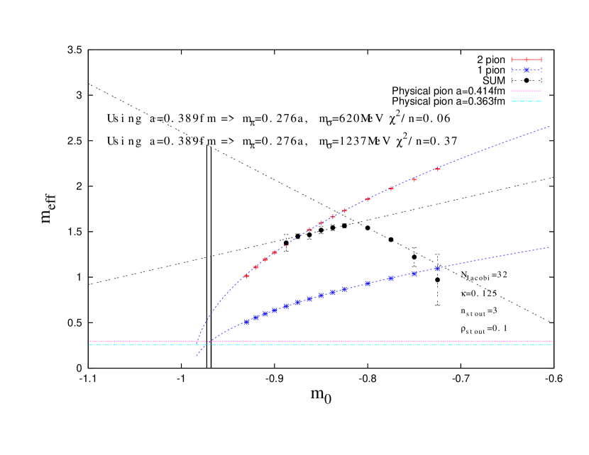
Figure 2: Effective masses, in lattice units, for the four-point correlation function (19) shown in black dots. For comparison, the two-pion mass $2m_{\pi}$ is plotted with red pluses and the single pion mass with blue splashes (color on-line). Extrapolations to the physical point (marked by vertical lines) are also shown, using both the high and low parts of the spectrum. It can be seen that the heavy quark mass regime extrapolates to a drastically different value, emphasizing the need to work at sufficiently small masses. The reasons behind the very different behavior in the two regimes is discussed in the main text.

4 Results

All of the results presented in this section are obtained with gauge coupling of $\beta=6/g^{2}=5.45$ and clover fermions with the tree-level improvement coefficient of $c_{\text{SW}}=1.0$. This is a quenched calculation, so the fermion determinant is set to unity in the simulation, which is performed with the standard $SU(3)$ heatbath [39]. 5000 thermalization sweeps were performed prior to sampling, and samples were separated by 200 sweeps. For all but the lightest pion mass, 4000-4500 samples were used in our expectation values. For the lightest mass, only 2000 samples were used, due to the cost of matrix inversion being significantly greater as the condition number increases. In order to address autocorrelations, the error estimates were based on a jackknife analysis with jackknife blocks of 400 samples. All data was obtained from $10^{3}\times 20$ lattices, which is why the coarse lattice spacing corresponding to $\beta=5.45$ was used ($a\sim 0.4$ fm). For the relatively large pion masses that we simulated, the finite volume effects are under control, with $m_{\pi}L\geq 4$.

As stated in the previous section, we were forced to omit the $C_{1}(t)$ contribution from our calculation due to the overwhelming amount of noise it introduces. We can expect reasonable results even with this omission as the numerical values of $C_{1}(t)$ are much larger than the other contributions, but exhibit little to no sign of exponential decay. On the other hand, we do include the partially disconnected diagram $C_{2}(t)$, which it has been argued in [40] is the most important one to include and should “never” be neglected (although several of the studies mentioned in the introduction do so).

Figure 2 shows the rest-mass energy of the ground state in the two-pion channel obtained from the correlation function

$$C_{\text{sum}}^{\prime}=C_{1}(t)-2C_{2}(t)$$ (19)

This estimate comes from the plateau in the effective mass for each of the bare quark masses included in our study. The prime in Eq. (19) indicates that the doubly disconnected diagram is omitted. It is a straightforward and standard calculation to compute the pion masses as a function of the bare mass $m_{0}a$, and determine the physical point once the lattice scale $a$ has been set.

Three traits can be observed from Fig. 2. First, for the lightest pion masses included in our study, with a corresponding bare mass $m_{0}a=-0.8875$, the extracted ground state energy is consistent with $2m_{\pi}$ within error bars. Second, for the other light masses, the effective mass exhibits a linear variation with bare mass and extrapolates to mass that is consistent with the expectations for the $f_{0}(500)$, given the uncertainties and systematic errors inherent in our study. Thus we identify this linear behavior, which is lighter than the corresponding $2m_{\pi}$, as a scalar state with quantum numbers $0^{++}$, the “would-be” resonance alluded to in our earlier discussions. Third, for the heavier pion masses, the effective mass diverges from the low mass linear trend, and extrapolates to a much larger mass at the physical point. The reason for this very different behavior is that in the heavy quark regime the single annihilation diagrams, Fig. 1(c), 1(d), begin to play an increasing role, and these are subtracted from the sum, according to Eq. (19). They become important because in this regime the quarks are very heavy so the the four propagators stretching over a long time interval in Fig. 1(a) are suppressed relative to only two such propagators in Fig. 1(c) and 1(d). Since these effect scale as different powers of $1/m$, where $m$ is the dressed quark mass, it increases as we go to heavier quarks.

We extrapolated the linear behaviour of the lighter masses (leaving out the lightest mass) down to the physical pion mass, obtaining an estimate of $M_{0^{++}}=609\pm 80$ MeV. This is significantly lighter than the $f_{0}(980)$, suggesting that the observed state is the ${f_{0}(500)}$ or $\sigma$. While this is somewhat heavier than the accepted value of 400-550 MeV [41], it is not inconsistent given our estimates of error. Furthermore, there is an unknown systematic error due to quenching (setting the fermion determinant to unity), and it is a large extrapolation, which could also introduce errors that may be unaccounted for. We have also extrapolated the heavier masses, illustrating that working in a heavy quark regime would lead to completely specious results, with $M_{0^{++}}=1237\pm 80$ MeV.

The physical scale $a$ was deduced by determining the Sommer parameter $r_{0}/a$ for our value of $\beta=5.45$ [42]. The exponential decay in Wilson loops with respect to the temporal extent was used to identify the values of the static quark potential $V(R)$. As usual, the Sommer parameter in lattice units was identified from setting $R^{2}dV(R)/dR|_{R=r_{0}/a}=1.65$ and taking $r_{0}=0.5$ fm to convert to physical units. We use two different prescriptions to identify the plateau, giving two estimates for the lattice spacing, 0.414 fm and 0.363 fm. We then use their mean to estimate physical mass, and the separation to estimate the scale setting error. This error is included in our uncertainties in the previous paragraph. Thus we have arrived at our estimated mass:

$$m_{\sigma}=609\pm 80~{}\text{MeV}.$$ (20)

This is consistent with a $\sigma$ to within errors and is not consistent with the other available state in this symmetry channel, the $f_{0}(980)$. We take encouragement from this exploratory result that the $\sigma$ can be identified on the lattice.

One question that arises is whether the state that we see at 609 MeV is a bound state or a multi-particle scattering state. These can be distinguished by examining the finite volume dependence of the extracted mass [43, 44, 45, 46]. If the state is a bound state, then the finite volume correction falls of exponentially, with the mass difference $M-2m_{\pi}$ rapidly approaching a constant. However, if the state is a scattering state, then $M-2m_{\pi}$ only falls of like $1/L^{3}$. We have measured the mass for a few of our $m_{0}a$ values on $L=10,12$ and $16$ lattices and find that it only varies by a few percent, lending support to the conclusion that the state we are looking at is a bound state, and not a scattering state. For instance for $m_{0}a=-0.875$, with Coulomb gauge fixed Jacobi smeared wall sources, we find $(M-2m_{\pi})a=0.045\pm 0.003$ for $L=10$ and $(M-2m_{\pi})a=0.070\pm 0.005$ for $L=16$. Thus, the mass difference is certainly not falling as $1/L^{3}$, and in fact increases somewhat. In more absolute terms, $M(10)a=1.483\pm 0.003$ and $M(16)a=1.508\pm 0.003$ so that the mass only changes by $1.6$% as we change the volume, certainly not consistent with a scattering state, and strongly supportive of a bound state.

5 Conclusions and further work

In this work we have shown that with a modest sized, quenched lattice, and a minimum of inversion overhead, one can identify a $0^{++}$ state that is signficantly lighter than the $f_{0}(980)$ at the physical point, which one would then naturally identify with $f_{0}(500)$. Though we omitted the doubly disconnected diagram (full annihilation) contribution $C_{1}(t)$, we included the singly connected contribution $C_{2}(t)$, following the recommendation of [40]. We emphasize that this was a very modest calculation by “modern” standards, and is illustrative of an alternative confirmational study that complements the much more demanding and thorough study of [16].

We collected this data using a Jacobi smeared wall source, which provides both the advantage of focusing the quark distribution around vanishing conjugate momentum, and suppression of UV and excited state contamination. This allowed us to avoid all-to-all propagators in the calculation of diagrams involving quark annihilation, with the modest GPU resources that were involved in this project; see Appendix C.

Future studies will repeat the study on larger lattice with a finer lattice spacing, and will also explore the region where the resonance is heavier than $2m_{\pi}$ by subtracting the two pion scattering state in a sequential Bayesian analysis [47]. We will also explore using the approximation (14) with a subset $Q$ that includes more momentum modes than ${\bf p}=0$. Furthermore, the current measurements will be extended to dynamical fermion lattices that we are currently generating. This will remove the unknown quenching errors from our study.

We note that an analysis of the spectrum of resonances using the phase shift has not been conducted in this study. This is an extremely demanding project requiring much larger resources than were available to our study here. In addition, sophistocated methods for handling annihilation diagrams, which greatly reduce the noise to signal ratio are required, such as distillation techniques that were employed in [16]. This sort of study has only recently been achieved, in a heroic effort [16]. Even with this very advanced approach, which has been over a decade in the making, the uncertainties on the lattice-derived properties (mass and width) of the $f_{0}(500)$ are quite large. It is our intention to perform such an analysis in the future, but we must first arrive at ways to improve upon the approach in the work that we have just cited. As computational resources head toward the exascale, we believe that it will be possible to accomplish this. However, we would like to emphasize that the study that we have performed is complementary to a phase shift analysis, and plays an important role, providing confirmation of the existence of the $f_{0}(500)$ state in lattice QCD by an alternative, much cheaper method.

Appendix A Non-gauge-invariant correlation functions

Here we want to consider what happens if we use operators that are not gauge invariant. What we will show is that the expectation value of such operators, or their correlation functions, will have a nonvanishing result if there is a singlet component in the decomposition with respect to the lattice gauge group. That is, non-gauge-invariant correlation functions generally transform in a reducible representation, which may or may not contain the singlet representation under a decomposition into irreducible representations. This is relevant to the considerations in the body of the paper above because when we use wall sources, but Fourier transform over sink locations, a singlet component emerges, which is the physical, gauge invariant correlation function that we are after. Note that this occurs without any gauge fixing, though the proof of this that now follows uses gauge fixing as an intermediate step to establish this fact. Here, we will closely follow the discussion of gauge fixing that is found in the classic monograph by Creutz [48].

Initially we will focus on the pure gauge theory. Considerations including quarks will only require a slight generalization. Our observable, or correlation function, is a functional $P[U]$ of the gauge links $\{U_{\mu}(x)\}\equiv\{U_{ij}\}$, where in the latter notation $i,j$ are neighboring sites. It is an identity that we can write

$$Z^{-1}\int[dU]e^{-S[U]}P[U]$$

$$=Z^{-1}\int\prod_{\{ij\}\in T}dg_{ij}\int[dU]\prod_{\{ij\}\in T}\delta(U_{ij},g_{ij})e^{-S[U]}P[U]$$ (21)

where $T$ represents a maximal tree, a maximal set of links that can be set to desired values $g_{ij}$ using lattice gauge invariance. Next we consider the effect of a gauge transformation

$$U_{ij}=g_{i}^{-1}U^{\prime}_{ij}g_{j}$$ (22)

under which the measure and action are invariant; the delta function also has a sort of invariance:

$$\delta(U_{ij},g_{ij})=\delta(g_{i}U_{ij}g_{j}^{-1},g_{i}g_{ij}g_{j}^{-1})=\delta(U^{\prime}_{ij},g_{i}g_{ij}g_{j}^{-1})$$ (23)

The resulting expression is then

$$Z^{-1}\int[dU]e^{-S[U]}P[U]$$

$$=Z^{-1}\int\prod_{\{ij\}\in T}dg_{ij}\int[dU^{\prime}]\prod_{\{ij\}\in T}\delta(U^{\prime}_{ij},g_{i}g_{ij}g_{j}^{-1})e^{-S[U]}P[\{g_{i}^{-1}U^{\prime}_{ij}g_{j}\}]$$ (24)

Now the point is that for the maximal tree, we can choose $\{g_{i}\}$ such that

$$g_{i}g_{ij}g_{j}^{-1}=\mathbb{I}$$ (25)

Then if the observable was gauge invariant, $P[\{g_{i}^{-1}U^{\prime}_{ij}g_{j}\}]=P[U^{\prime}]$, the $g_{ij}$ dependence disappears and the integration over this set of group elements just yields an inconsequential factor, so that the correlation function with the fixed links is equivalent to the original one without any gauge fixing. On the other hand, if the observable is not gauge invariant, we apply the rules of group integration to see the effect of integration over group orbits. For instance, suppose a plaquette observable but without the trace:

$$P[U]=U_{ij}U_{jk}U_{kl}U_{li}$$ (26)

where the indices are only site indices; color indices are suppressed; the gauge invariant observable is $\mathop{{\hbox{Tr}\,}}\nolimits P[U]$. In this case, the integral is

$$Z^{-1}\int\prod_{\{ij\}\in T}dg_{ij}\int[dU^{\prime}]\prod_{\{i^{\prime}j^{\prime}\}\in T}\delta(U^{\prime}_{i^{\prime}j^{\prime}},\mathbb{I})e^{-S[U]}g_{i}^{-1}U^{\prime}_{ij}U_{jk}U_{kl}U_{li}g_{i}$$ (27)

The $g_{i}$ that appear here are determined by the $\{g_{ij}\}$ and they will be integrated over with the group invariant measure. Then the identity

$$\int dG~{}G_{\alpha\beta}G^{\dagger}_{\gamma\delta}=\delta_{\alpha\gamma}\delta_{\beta\delta}$$ (28)

where $\alpha,\beta,\ldots$ are color indices, will project out the trace of the plaquette.

Addition of fermions to this discussion is straightforward. The action remains invariant, but the operator $P[U]$ will now include factors of $M^{-1}[U]$. If $P[U]$ is a correlation function that is not gauge invariant, only the singlet part of the decomposition will survive the integral over gauge orbits that is inherent in a Monte Carlo simulation. Since the Fourier transform of the correlation function built from wall sources will necessarily involve contributions that are ultralocal, i.e., gauge singlets, we will obtain a nonvanishing answer.

Appendix B Smeared wall sources

Empirically, smearing a wall source significantly reduces excited state contamination. This can be seen in Fig. 3, which shows the pion effective mass plot with and without smearing, using wall sources, for two different values of the bare mass.

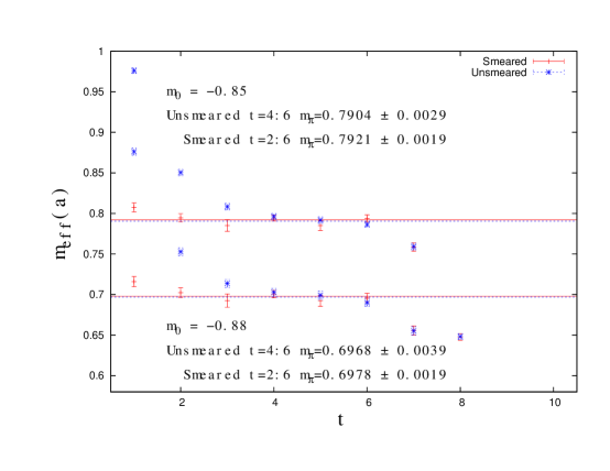
Figure 3: Pion effective mass for two values of the bare mass. The upper data corresponds to $m_{0}a=-0.85$ and the lower data to $m_{0}a=-0.88$. All quantities are in lattice units. This plot compares wall sources with and without Jacobi smearing. It can be seen that the plateau is achieved significantly earlier when smearing is used.

One can ask why this is successful. After all, one expects that for these relatively heavy pions the dominant modes would be quarks at rest, which is what wall sources create, i.e., ${\bf p}=0$. However, it is important to note that the conjugate momentum is not ${\bf p}$, but is $\boldsymbol{\pi}\equiv{\bf p}+{\bf A}$. Jacobi smearing applies $e^{\alpha{\tilde{\nabla}}^{2}}$ to the ${\bf p}=0$ source, which in momentum space becomes $e^{-\alpha\boldsymbol{\pi}^{2}}$. In a general gauge background ${\bf p}=0$ does not correspond to the mode with vanishing conjugate momentum. The ground state has the strongest overlap with $\boldsymbol{\pi}=0$ modes, and the Jacobi smearing amends the source with link fields in such a way that this is predominantly what is contained in the resulting operator. This is why smearing ${\bf p}=0$ sources improves the ground state signal.

Appendix C GPU acceleration

As part of our NSF funded project, we developed a clover fermion interface between the Columbia Physics System and QUDA, where the latter is a GPU library for lattice QCD [49]. This allows us to take advantage of a lattice QCD application library (CPS), as well as GPU acceleration for all of our inversions. We have fully validated that our fermion matrix multiplication and inversions agree between the native CPS routines and the ones obtained through our QUDA interface. Our code is available for public use at https://github.com/cpviolator, or upon request. Our code was largely run on XSEDE resources [50] for this study, with various supplementary allocations and resources for side studies and analysis.

References

- [1] G. Grayer, B. Hyams, C. Jones, P. Schlein, P. Weilhammer, et al., High Statistics Study of the Reaction pi- p –¿ pi- pi+ n: Apparatus, Method of Analysis, and General Features of Results at 17-GeV/c, Nucl.Phys. B75 (1974) 189.
- [2] GAMS NA12/2 Collaboration, T. Ishida, T. Kinashi, H. Shimizu, K. Takamatsu, and T. Tsuru, Study of the pi0 pi0 system below 1-GeV region in the p p central collision reaction at 450-GeV/c, in Manchester 1995, Proceedings, Hadron ’95, p. 451, 1995.
- [3] E852 Collaboration, J. Gunter et al., A Partial wave analysis of the pi0 pi0 system produced in pi- p charge exchange collisions, Phys.Rev. D64 (2001) 072003, [hep-ex/0001038].
- [4] BES Collaboration, M. Ablikim et al., The sigma pole in J / psi —¿ omega pi+ pi-, Phys.Lett. B598 (2004) 149–158, [hep-ex/0406038].
- [5] C. E. Detar and J. B. Kogut, Measuring the Hadronic Spectrum of the Quark Plasma, Phys.Rev. D36 (1987) 2828.
- [6] W.-J. Lee and D. Weingarten, Scalar quarkonium masses and mixing with the lightest scalar glueball, Phys.Rev. D61 (2000) 014015, [hep-lat/9910008].
- [7] UKQCD Collaboration, C. Michael, M. Foster, and C. McNeile, Flavor singlet pseudoscalar and scalar mesons, Nucl.Phys.Proc.Suppl. 83 (2000) 185–187, [hep-lat/9909036].
- [8] M. G. Alford and R. Jaffe, Insight into the scalar mesons from a lattice calculation, Nucl.Phys. B578 (2000) 367–382, [hep-lat/0001023].
- [9] UKQCD Collaboration Collaboration, C. McNeile and C. Michael, Mixing of scalar glueballs and flavor singlet scalar mesons, Phys.Rev. D63 (2001) 114503, [hep-lat/0010019].
- [10] SCALAR Collaboration Collaboration, T. Kunihiro et al., Scalar mesons in lattice QCD, Phys.Rev. D70 (2004) 034504, [hep-ph/0310312].
- [11] UKQCD Collaboration Collaboration, A. Hart, C. McNeile, C. Michael, and J. Pickavance, A Lattice study of the masses of singlet 0++ mesons, Phys.Rev. D74 (2006) 114504, [hep-lat/0608026].
- [12] S. Prelovsek and D. Mohler, A Lattice study of light scalar tetraquarks, Phys.Rev. D79 (2009) 014503, [arXiv:0810.1759].
- [13] S. Prelovsek, T. Draper, C. B. Lang, M. Limmer, K.-F. Liu, et al., Lattice study of light scalar tetraquarks with : Are and tetraquarks?, Phys.Rev. D82 (2010) 094507, [arXiv:1005.0948].
- [14] G. P. Engel, C. Lang, M. Limmer, D. Mohler, and A. Schafer, QCD with two light dynamical chirally improved quarks: Mesons, Phys.Rev. D85 (2012) 034508, [arXiv:1112.1601].
- [15] M. Wakayama, Structure of the sigma meson from lattice QCD, PoS Hadron2013 (2014) 106.
- [16] R. A. Briceno, J. J. Dudek, R. G. Edwards, and D. J. Wilson, Isoscalar scattering and the meson resonance from QCD, Phys. Rev. Lett. 118 (2017), no. 2 022002, [arXiv:1607.0590].
- [17] TXL, TkL Collaboration, G. Bali et al., Glueballs and string breaking from full QCD, Nucl.Phys.Proc.Suppl. 63 (1998) 209–211, [hep-lat/9710012].
- [18] LHCb Collaboration, R. Aaij et al., Measurement of the resonant and CP components in decays, Phys.Rev. D90 (2014), no. 1 012003, [arXiv:1404.5673].
- [19] B. Hyams, C. Jones, P. Weilhammer, W. Blum, H. Dietl, et al., Phase Shift Analysis from 600-MeV to 1900-MeV, Nucl.Phys. B64 (1973) 134–162.
- [20] T. Ishida, On Existence of sigma (555) particle: Study in p p central collision reaction and reanalysis of pi pi scattering phase shift, .
- [21] F. Yndurain, R. Garcia-Martin, and J. Pelaez, Experimental status of the pi pi isoscalar S wave at low energy: f(0)(600) pole and scattering length, Phys.Rev. D76 (2007) 074034, [hep-ph/0701025].
- [22] I. Caprini, Finding the sigma pole by analytic extrapolation of pi pi scattering data, Phys.Rev. D77 (2008) 114019, [arXiv:0804.3504].
- [23] S. Okubo, Phi meson and unitary symmetry model, Phys.Lett. 5 (1963) 165–168.
- [24] G. Zweig, An SU(3) model for strong interaction symmetry and its breaking. Version 2, .
- [25] M. Ishida, Possible classification of the chiral scalar sigma nonet, Prog.Theor.Phys. 101 (1999) 661–669, [hep-ph/9902260].
- [26] K. Yamawaki, Conformal Higgs, or techni-dilaton- composite Higgs near conformality, Int.J.Mod.Phys. A25 (2010) 5128–5144, [arXiv:1008.1834].
- [27] R. L. Jaffe, Multi-Quark Hadrons. 1. The Phenomenology of (2 Quark 2 anti-Quark) Mesons, Phys.Rev. D15 (1977) 267.
- [28] R. L. Jaffe, Multi-Quark Hadrons. 2. Methods, Phys.Rev. D15 (1977) 281.
- [29] R. Gupta, A. Patel, and S. R. Sharpe, I = 2 pion scattering amplitude with Wilson fermions, Phys.Rev. D48 (1993) 388–396, [hep-lat/9301016].
- [30] J. Foley, K. Jimmy Juge, A. O’Cais, M. Peardon, S. M. Ryan, et al., Practical all-to-all propagators for lattice QCD, Comput.Phys.Commun. 172 (2005) 145–162, [hep-lat/0505023].
- [31] Hadron Spectrum Collaboration, M. Peardon et al., A Novel quark-field creation operator construction for hadronic physics in lattice QCD, Phys.Rev. D80 (2009) 054506, [arXiv:0905.2160].
- [32] C. Morningstar, J. Bulava, J. Foley, K. J. Juge, D. Lenkner, et al., Improved stochastic estimation of quark propagation with Laplacian Heaviside smearing in lattice QCD, Phys.Rev. D83 (2011) 114505, [arXiv:1104.3870].
- [33] J. Giedt and D. Howarth, Stochastic propagators for multi-pion correlation functions in lattice QCD with GPUs, arXiv:1405.4524.
- [34] D. Howarth and J. Giedt, Scalar Mesons on the Lattice Using Stochastic Sources on GPU Architecture., PoS LATTICE2014 (2014) 096.
- [35] M. Gockeler, R. Horsley, H. Oelrich, H. Perlt, P. E. Rakow, et al., Lattice renormalization of quark operators, Nucl.Phys.Proc.Suppl. 63 (1998) 868–870, [hep-lat/9710052].
- [36] M. Gockeler, R. Horsley, H. Oelrich, H. Perlt, D. Petters, et al., Nonperturbative renormalization of composite operators in lattice QCD, Nucl.Phys. B544 (1999) 699–733, [hep-lat/9807044].
- [37] C. Morningstar and M. J. Peardon, Analytic smearing of SU(3) link variables in lattice QCD, Phys. Rev. D69 (2004) 054501, [hep-lat/0311018].
- [38] G. M. von Hippel, B. J ger, T. D. Rae, and H. Wittig, The Shape of Covariantly Smeared Sources in Lattice QCD, JHEP 1309 (2013) 014, [arXiv:1306.1440].
- [39] N. Cabibbo and E. Marinari, A New Method for Updating SU(N) Matrices in Computer Simulations of Gauge Theories, Phys.Lett. B119 (1982) 387–390.
- [40] F.-K. Guo, L. Liu, U.-G. Meissner, and P. Wang, Tetraquarks, hadronic molecules, meson-meson scattering and disconnected contributions in lattice QCD, Phys.Rev. D88 (2013) 074506, [arXiv:1308.2545].
- [41] Particle Data Group Collaboration, K. Olive et al., Review of Particle Physics, Chin.Phys. C38 (2014) 090001.
- [42] R. Sommer, A New way to set the energy scale in lattice gauge theories and its applications to the static force and alpha-s in SU(2) Yang-Mills theory, Nucl.Phys. B411 (1994) 839–854, [hep-lat/9310022].
- [43] H. W. Hamber, E. Marinari, G. Parisi, and C. Rebbi, Considerations on Numerical Analysis of QCD, Nucl. Phys. B225 (1983) 475.
- [44] M. Luscher, Volume Dependence of the Energy Spectrum in Massive Quantum Field Theories. 1. Stable Particle States, Commun.Math.Phys. 104 (1986) 177.
- [45] M. Luscher, Volume Dependence of the Energy Spectrum in Massive Quantum Field Theories. 2. Scattering States, Commun.Math.Phys. 105 (1986) 153–188.
- [46] M. Luscher, Two particle states on a torus and their relation to the scattering matrix, Nucl.Phys. B354 (1991) 531–578.
- [47] Y. Chen, S.-J. Dong, T. Draper, I. Horvath, K.-F. Liu, N. Mathur, S. Tamhankar, C. Srinivasan, F. X. Lee, and J.-b. Zhang, The Sequential empirical bayes method: An Adaptive constrained-curve fitting algorithm for lattice QCD, hep-lat/0405001.
- [48] M. Creutz, Quarks, gluons and lattices. Cambridge Monographs on Mathematical Physics. Cambridge Univ. Press, Cambridge, UK, 1985.
- [49] M. Clark, R. Babich, K. Barros, R. Brower, and C. Rebbi, Solving Lattice QCD systems of equations using mixed precision solvers on GPUs, Comput.Phys.Commun. 181 (2010) 1517–1528, [arXiv:0911.3191].
- [50] J. Towns, T. Cockerill, M. Dahan, I. Foster, K. Gaither, A. Grimshaw, V. Hazlewood, S. Lathrop, D. Lifka, G. D. Peterson, R. Roskies, J. R. Scott, and N. Wilkins-Diehr, Xsede: Accelerating scientific discovery, Computing in Science & Engineering 16 (2014), no. 5 62–74.