A Sard theorem for graph theory

Abstract.

The zero locus of a function $f$ on a graph $G$ is defined as the graph for which the vertex set consists of all complete subgraphs of $G$, on which $f$ changes sign and where $x,y$ are connected if one is contained in the other. For $d$-graphs, finite simple graphs for which every unit sphere is a $d$-sphere, the zero locus of $(f-c)$ is a $(d-1)$-graph for all $c$ different from the range of $f$. If this Sard lemma is inductively applied to an ordered list functions $f_{1},\dots,f_{k}$ in which the functions are extended on the level surfaces, the set of critical values $(c_{1},\dots,c_{k})$ for which $F-c=0$ is not a $(d-k)$-graph is a finite set. This discrete Sard result allows to construct explicit graphs triangulating a given algebraic set. We also look at a second setup: for a function $F$ from the vertex set to $R^{k}$, we give conditions for which the simultaneous discrete algebraic set $\{F=c\}$ defined as the set of simplices of dimension $\in\{k,k+1,\dots,n\}$ on which all $f_{i}$ change sign, is a $(d-k)$-graph in the barycentric refinement of $G$. This maximal rank condition is adapted from the continuum and the graph $\{F=c\}$ is a $(n-k)$-graph. While now, the critical values can have positive measure, we are closer to calculus: for $k=2$ for example, extrema of functions $f$ under a constraint $\{g=c\}$ happen at points, where the gradients of $f$ and $g$ are parallel $\nabla f=\lambda\nabla g$, the Lagrange equations on the discrete network. As for an application, we illustrate eigenfunctions of $d$-graphs and especially the second eigenvector of $3$-spheres, which by Courant-Fiedler has exactly two nodal regions. The separating nodal surface of the second eigenfunction $f_{1}$ always appears to be a 2-sphere in experiments. By Jordan-Schoenfliess, both nodal regions would then be 3-balls and the double nodal curve $\{f_{1}=0,f_{2}=0\}$ would be an un-knotted curve in the 3-sphere. Graph theory allows to approach such unexplored concepts experimentally, as the corresponding question are open even classically for nodal surfaces of the ground state of the Laplacian of a Riemannian $3$-sphere $M$.

1. Introduction

We explore vector-valued functions $F$ on the vertex set of a finite simple graph $G=(V,E)$. Most of the notions introduced here are defined for general finite simple graphs. But as we are interested in Lagrange extremization, Morse and Sard type results in graph theory as well as questions in the spectral theory of the Laplacian on graphs related to Laplacians of Riemannian manifolds, we often assume $G$ to be a $d$-graph, which is a finite simple graph, for which all unit spheres are $(d-1)$-spheres in the sense of Evako [KnillJordan]. In a first setup, more suited for Sard, for all except finitely many choices of $c\in R^{d}$, the graph $\{F=c\}=\{f_{1}=c_{1},\dots,f_{k}=c_{k}\}$ is a $(d-k)$-graph, in a second setup, closer to classical calculus, we need to satisfy locally a maximal rank condition to assure that the graph representing the discrete algebraic set $\{F=c\}$ is a $(d-k)$-graph.

The first part of the story parallels classical calculus and deals with the concept of level surface. It starts with a pleasant surprise when looking at a single function: there is a strong Sard regularity for a $d$-graph $G$: given a hyper-surface $G_{f}(x)=\{f=c\}$ defined as the graph with vertex set consisting of all simplices on which $f-c$ changes sign, the graph $\{f=c\}$ is a $(d-1)$-graph if $c$ is not a value taken by $f$. The topology of $G_{f}(c)$ changes only for parameter values $c$ contained in the finite set $f(V)$. This observation was obtained when studying coloring problems [knillgraphcoloring, knillgraphcoloring2, KnillNitishinskaya], as a locally injective function on the vertex set is the same than a vertex coloring. Before, in [indexexpectation, indexformula], we just looked at the edges, on which $f$ changes sign and then completed the graph artificially. Now, we have this automatic. We hope to apply this to investigate nodal regions of eigenfunctions of the Laplacian of a graph, where we believe the answers to be the same for compact $d$-dimensional Riemannian manifolds or finite $d$-graphs. With the context of level surfaces one has the opportunity to look at nodal surfaces of eigenfunctions, which are also known as Chladni surfaces bounding nodal regions.

With more than one function, the situation changes as the singular set typically becomes larger in the discrete. This is where the story splits. In the commutative setup, where we look at the zero locus of all functions simultaneously, Sard fails, while in the setup, where an ordered set of functions is considered, Sard will be true: as in the classical Sard theorem [Morse1939, Sard1942], the set of critical values has zero measure. The difference already is apparent if we take two random functions on a discrete $3$-sphere for example. Then simultaneous level set $\{f=0,g=0\;\}$ is a graph without triangles but it is rarely a $1$-graph, a finite union of circular graphs. The reason is that the tangent space is a finite set and the probability of having two parallel gradients at a vertex does not have zero probability. However, if we look at $g=0$ on the two dimensional surface $f=0$, we get a finite union of cyclic graphs. In general, we salvage regularity and Sard by defining the algebraic set $\{F=c\}$ in a different way by recursively building hyper surfaces: start with the hyper surface $\{f_{1}=c_{1}\}$, then extend $f_{2}$ to the new graph and look at $\{f_{2}=c_{2}\}$ inside $\{f_{1}=c_{1}\}$. Now a vector value $c\in R^{k}$ is always regular if $c$ is not in the image of $F$ applied to recursively defined graph. This is the discrete analog of the multi-dimensional Sard theorem in classical analysis. The order in which the functions are taken, matters in the discrete. But this is not a surprise as we refine in each step the graph and therefore have to extend the functions to the barycentric refinements. Its only for sufficiently smooth functions like eigenfunctions of low energy eigenvalues of the graph that the answer can be expected to be independent of the ordering.

The graph theoretical approach is useful for making experiments: take a 3-graph $G=(V,E)$ for example and take two real valued functions $f,g$ on the vertex set $V$. If $c$ is not in the image of $f$, we can look at the level surface $f=c$ and extend $g$ to a function there (vertices are now simplices and we just average the function value $g$ to extend the function). If $d$ is not in the image of $g$, then the $1$-graph $Z=\{g=d\}$ is a subgraph of $\{f=c\}$. It is a finite set of closed curves in $G_{2}$. In other words, each connected component is a knot in the 3-sphere. Unlike in the continuum, we do not have to worry about cases, where the knot intersects or self intersects. The Sard theorem assures that this will never happen in the discrete. We only have to assure that the value $c$ is not in $f(V)$ and $d$ is not in $g(V)$.

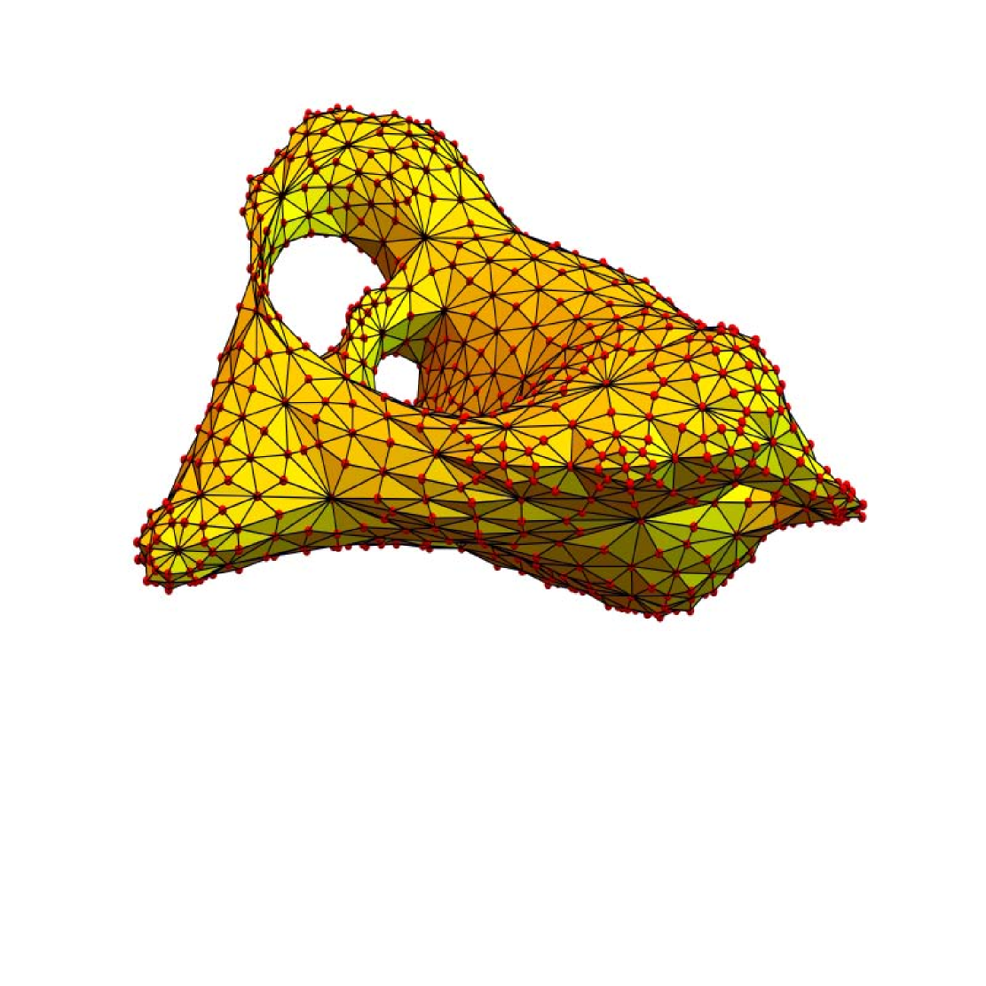
Figure 1. We see an example of a level surface $G_{f}(c)=\{f=c\}$ in a 3-sphere $G$. The graph $G$ is a Barycentric refinement of a 3D octahedron with 8 vertices with simplex cardinalities $\vec{v}=(80,464,768,384)$ satisfying $\chi(G)=\sum_{i}(-1)^{i}v_{i}=0$. The zero Euler characteristic is a property shared by all 3-graphs like 3-manifolds. The graph $G$ admits an involution $T$ such that $G/T$ is a discrete projective 3-space. The algebraic level set $G_{f}(c)$ displayed here is a $2$-graph, a two-dimensional surface within the Barycentric refinement $G_{1}$ of $G$. The ambient sphere $G_{1}$ already has $1696$ vertices and $10912$ edges and $18432$ triangles, $9216$ tetrahedra. The surface $\{f=c\}$ is a discrete analogue of a $2$-dimensional projective variety. By the Sard lemma, the level sets $G_{f}(c)=\{f=c\}$ are always nonsingular if $c\notin f(V)$. Furthermore the surface $G_{f}(c)$ is $4$-colorable.

The second setup, which defines discrete algebraic sets $Z=\{f_{1}=c_{1},\dots,f_{k}=c_{k}\}$ in the Barycentric refinement $G_{1}$ of $G$ requires a few definitions. We need conditions under which these sets are nonsingular in the sense that they again form a $(d-k)$-graph, graphs for which the unit sphere $S(x)$ is a sphere at every vertex. In general, the situation is the same as in the continuum, where varieties are not necessarily manifolds. The definition is straightforward: define $\{F=c\;\}$ as the set of simplices of dimension in $\{k,\dots,n\}$ in $G$ on which all functions $f_{j}$ change sign simultaneously. The graph $\{F=c\}$ is a subgraph of the Barycentric refinement $G_{1}=G\times 1$ of $G$. Conditions for regularity could be formulated locally in terms of spheres in spheres. In some sense, a locally projective tangent bundle with discrete projective spaces associated to unit spheres replaces the tangent bundle. It is still possible to define a vector space structure at each point and define a discrete gradient $\nabla f$ of a function. If $G$ is a $d$-graph, $x$ is a complete $K_{d+1}$ subgraph, then $\nabla f(x,x_{0})$ is defined as the vector $\nabla f=\langle{\rm sign}(f(x_{1})-f(x_{0})),\dots,{\rm sign}(f(x_{d})-f(x_{0}))\rangle$. The local injectivity condition means that $\nabla f(x,x_{0})$ is not zero for all $d$-simplices containing $x_{0}$. This leads to the Sard Lemma (1). But now, when changing $c$, we also need to look at the values $c_{i}=f(x_{i})$ taken by the function $f$ and investigate whether they are critical. What happens if $c$ passes a value $c_{i}=f(x_{i})$? If $f<c_{i}$ is homotopic to $f\leq c_{i}$, then the set $\{f=c\}\cap S(x)$ is a $(d-1)$-sphere which by Jordan-Brower-Schoenflies [KnillJordan] divides $S(x)$ into two complementary balls $S^{-}(x)$, $S^{+}(x)$. The Poincaré-Hopf index $1-\chi(S^{-}(x))=i_{f}(x)$ [poincarehopf] is then zero. At a local minimum of $f$ for example, the graph $S^{-}(x)$ is empty so that the index is $1$. At a local maximum, $S^{+}(x)$ is empty and the index is either $1$ or $-1$ depending on whether the dimension of $G$ is even or odd. In two dimensions, where we look at discrete multi-variable calculus, maxima and minima have index $1$ and saddle points have index $-1$.

The set of hypersurfaces $M_{j}=\{f=c_{j}\}$ form a contour map for which the individual leaves in general have different homotopy types. Topological transitions can happen only at values $f(V)$ of $f$ on the vertex set $V$ of the graph. We can relate the symmetric index $j_{f}(x)=[i_{f}(x)+i_{-f}(x)]/2$ at a vertex $x$ of $G$ with the $(d-2)$-dimensional graph $\{f=c_{k}\}$ in the unit sphere $S(x)$. We have called this the graph $B_{f}(x)$ and showed that the graph can be completed to become a $d$-graph. This completion can be done now more elegantly. As pointed out in [eveneuler], for $d=4$ for example, we get for every locally injective function $f$ a $2$-dimensional surface $B_{f}$, the disjoint union of $B_{f}(x)$. We see that a function $f$ not only defines $(d-1)$-graphs $G_{f}(c)=\{f=c\}$ but also $(d-2)$-graphs $B_{f}(x)$ called “central surfaces” for every vertex $x$.

If we have more than one function as constraints, the singularity structure of $\{f_{1}=c_{1},\dots,f_{k}=c_{k}\;\}$ is more complicated and resembles the classical situation, where singularities can occur. Also the Lagrange setup, where we mazimize or minimize functions under constraints, is very similar to the classical situation. The higher complexity entering with 2 or more functions is no surprise as also for classical algebraic sets defined as the zero locus of finitely many polynomials, the case of several functions is harder to analyze. In calculus, when studying extrema of a function $f$ under constraints $g$, following Lagrange, one is interested in critical points of $f$ and $g$ as well as places, where the gradients are parallel. Lets assume that we have two functions $f,g$ on the vertex sets of a geometric graph. The intersection $\{f=c,g=d\}$ with $S(x)$ is then a sphere of co-dimension $2$. If we have $2$ constraints and $G$ is $4$-dimensional for example, then $S(x)$ is a $3$-sphere and $S(x)\cap\{F=0\}$ is a knot inside $S(x)$. This can already be complicated. By triangulating Seifert surfaces associated by a knot, one can see that any knot can occur as a co-dimension $2$ curve of a graph. Briskorn sphere examples allow to make this explicit in the case of torus knots. With more than one function, Poincaré-Hopf indices form a discrete $1$-form valued grid because changing any of the $c_{j}$ can change the Euler characteristic. This allows to express the Euler characteristic as a discrete line integral in the discrete target set of $F$. There are now many Poincaré-Hopf theorems, for every deformation path, there is one.

If we look at the set $F=c$, where all functions change sign, singular values for $F=(f_{1},\dots,f_{k})$ are vectors $c=(c_{1},\dots,c_{k})$ in $R^{k}$ for which the graph $\{F=c\}$ is not a $(d-k)$-graph or values $c=F(x)$ taken on by $F$ on vertices $x$. Lets look at the very special example, where all $f_{j}$ are the same function. Now, near the diagonal $c_{i}=c$, there is an entire neighborhood of parameter values, where regularity fails. We see that the Sard statement does not hold in this commutative setting. We therefore also look at the non-commutative setup, where we fix $f_{1}=c_{1}$ first, then look at the level surface $\{f_{2}=c_{2}\}$ on the surface $\{f_{1}=c_{1}\}$ and proceed inductively. Sard is now more obvious, but the sets $F=0$ depend on the order, in which the functions $f_{j}$ have been chosen. This order dependence is no surprise in a quantum setting, if we look at $f_{j}$ as observables. It simply depends in which order we measure and fix the $f_{j}$.

There are analogies to Morse theory in the continuum: in the case of one single function, we can single out a nice class of graphs and functions, which lead to a discrete Morse theory. The geometric graph $G$ as well as functions on vertices are the only ingredients. One can now assign a Morse index $m(x)$ at a critical point and have $i_{f}(x)=(-1)^{m(x)}$. The requirement is an adaptation of a reformulation of the definition of being Morse means in the continuum that for a small sphere $S(x)$, the set $S(x)\cap\{f(y)=f(x)\}$ is a product $S_{m-1}\times S_{d-1-m}$. For example for $m=1,d=2$, we have a saddle point, where $S(x)$ intersects the level surface in $4$ points forming $S_{0}\times S_{0}$. In the enhanced picture, where we look at the graph $G_{1}$, we have this regularity more likely. One can extend the function to the new graph and repeat until one get a Morse function.

We can use graphs described by finitely many equations in order to construct examples of graphs to illustrate classical calculus like Stokes or Gauss theorem or surfaces to illustrate classical multivariable calculus. The notion of $d$-graphs has evolved from [elemente11, indexexpectation, eveneuler, knillgraphcoloring] to [knillgraphcoloring2], where it reached its final form. While finishing up [KnillJordan] a literature search showed that spheres had been defined in a similar way already by Evako earlier on.

The enhanced Barycentric refinement graph $G_{1}=G\times K_{1}$ is a regularizes graph which helps to study Jordan-Brouwer questions in graph theory [KnillJordan] and introduce a product structure on graphs which is compatible with cohomology [KnillKuenneth]. It also illustrates the Brouwer fixed point theorem [brouwergraph], as the fixed simplices on $G$ can be seen as fixed points on $G_{1}$. The simplex picture is also useful as the Dirac operator $D=d+d^{*}$ on a graph builds on it [DiracKnill, knillmckeansinger]. The graph spectra of successive Barycentric refinements converges universally, only depending on the size of the largest complete subgraph [KnillBarycentric].

An other application of the present Sard analysis is a simplification of [indexformula] which assures that the curvature $K$ is identically zero for $d=(2m+1)$-dimensional geometric graphs: write the symmetric index $j_{f}(x)=i_{f}(x)+i_{-f}(x)$ in terms of the Euler characteristic of the $(d-2)$-dimensional graph $G_{f}(x)$ obtained by taking the hypersurface $\{y\;|\;f(y)=f(x)\}$ in the unit sphere $S(x)$. For odd-dimensional geometric $d$-graphs, this symmetric index is is $-\chi(B_{f}(x))/2=j_{f}(x)$, while for even-dimensional graphs, it is $1-\chi(B_{f}(x))/2=j_{f}(x)$. One of the corollaries given here is that if $f$ is locally injective, then $B_{f}(x)$ is always a geometric $(d-2)$-graph if $G$ is a $d$-graph. In [indexexpectation], we called the uncompleted graphs polytopes and showed that one can complete them. Now, since the expectation of $j_{f}(x)$ is curvature, [indexexpectation, colorcurvature], this gives an immediate proof that odd-dimensional $d$-graphs have constant $0$ curvature. Zero curvature follows for odd-dimensional graphs. The regularity allows to interpret Euler curvature as an average of two-dimensional sectional curvatures. Euler characteristic written as the expectation of these sectional curvature averages is close to Hilbert action. It shows that the quantized functional “Euler characteristic” is not only geometrically relevant but that it has physical potential.

2. Level surfaces

The study of level surfaces $\{f=c\}$ in a graph is not only part of discrete differential topology. It belongs already to discretized multivariable calculus, where surfaces $\{f(x,y,z)=0\}$ in space or curves $\{f(x,y)=0\}$ in the plane are central objects. Some would call calculus on graphs “quantum calculus”. We want to understand under which conditions a sequence of $k$ real valued functions $F=(f_{1},\dots,f_{k})$ on the vertex set of a graph leads to co-dimension $k$ graphs $\{F=0\}$. We start with the case $k=1$, where we have a level surface $\{f=c\}$.

Definition 1.

Given a finite simple graph $G=(V,E)$, define the level hyper surface $\{f=c\}$ as the graph $G^{\prime}=(V^{\prime},E^{\prime})$ for which the vertex set $V^{\prime}$ is the set of simplices $x$ in $G$, on which the function $f-c$ changes sign in the sense that there are vertices in $x$ for which $f-c<0$ and vertices in $x$ for which $f-c>0$. A pair of simplices $(x,y)\in V^{\prime}\times V^{\prime}$ is in the edge set $E^{\prime}$ of $G^{\prime}$ if $x$ is a subgraph of $y$ or if $y$ is a subgraph of $x$. In the case $c=0$, the graph $\{f=0\}$ is also called the zero locus of $f$.

Remarks.
1) Instead of taking a real-valued function, we could take a function taking values in an ordered field. We need an ordering as we need to tell, where a function “changes sign”.
2) Most of the time we will assume $c$ is not a value taken by $f$. An alternative would be to include all simplices which contain a vertex on which $f=0$.

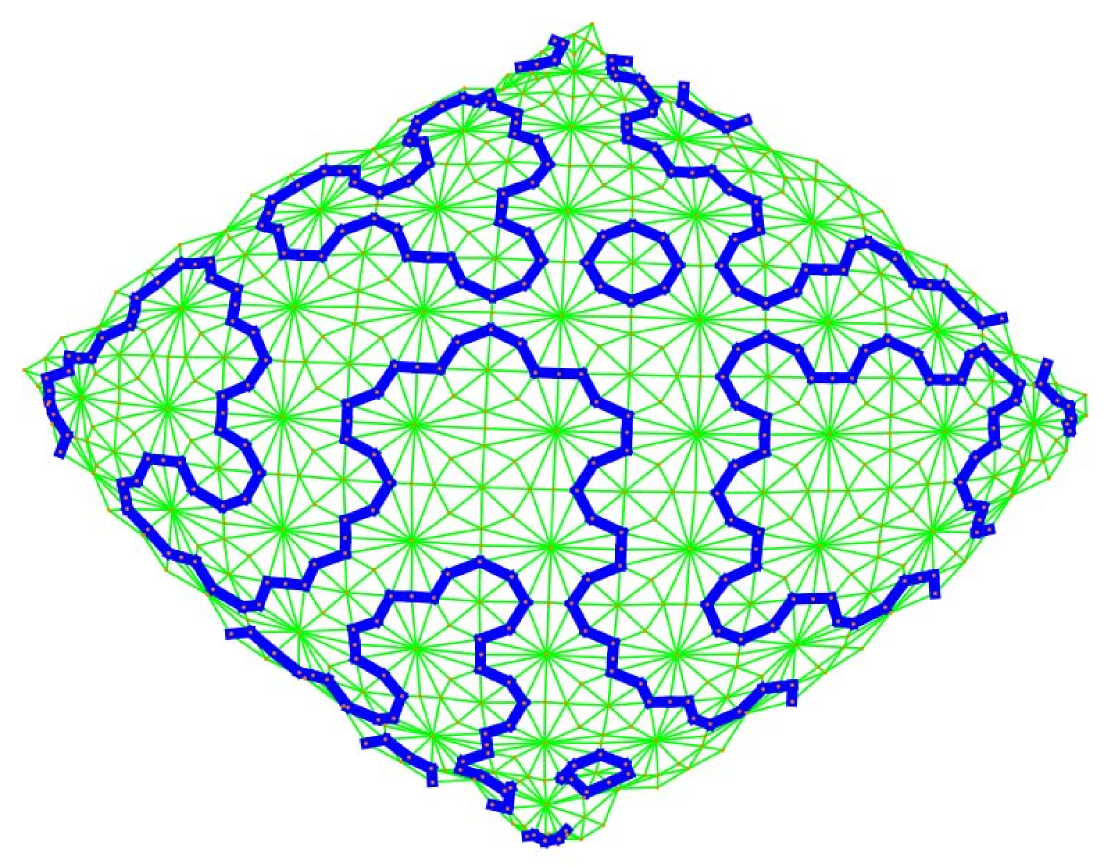
Figure 2. A level curve in a planar graph. A level surface in a 3-sphere.

Examples.
1) Let $G$ be a $2$-sphere like for example an icosahedron. Let $f$ be $1$ on exactly one vertex $x$ (a discrete Dirac delta function) and $0$ everywhere else. Now $\{f=1/2\}$ consists of all edges and triangles containing $x$. They form a circular graph and $\{f=0\}=C_{2{\rm deg}(x)}$.
2) Let $G=C_{n}\times C_{n}\times C_{n}$ be a discrete $3$-torus and let $f$ be a function which is $1$ on a circular closed graph and $0$ else. Then $\{f=1/2\}$ is a $2$-dimensional torus.

3. The Sard lemma

The following definitions are recursive and were first put forward by Evako. See [KnillJordan] for our final version.

Definition 2.

A $d$-sphere is a finite simple graph for which unit sphere $S(x)$ is a $(d-1)$-sphere and such that removing a single vertex from the graph renders the graph contractible. Inductively, a graph is contractible, if there exists a vertex such that both $S(x)$ and the graph generated with vertices without $x$ are contractible.

Definition 3.

A $d$-graph $G$ is a finite simple graph for which every unit sphere $S(x)$ is a $(d-1)$-sphere.

Examples.
1) A $1$-graph is a finite union of circular graphs, for which each connectivity component has $4$ or more vertices.
2) The icosahedron and octahedron graphs are both $2$-graphs. In the first case, the unit spheres are $C_{5}$, in the second case, the unit spheres are $C_{4}$.
3) In [KnillEulerian] we have classified all Platonic d-graphs using Gauss Bonnet [cherngaussbonnet]. Inductively, a $d$-graph $G$ is called Platonic, if there exists a $(d-1)$-graph $H$ which is Platonic such that all unit spheres of $G$ are isomorphic to $H$. In dimension $d=3$, there are only two Platonic graphs, the 16 and 600 cell. In dimensions $d\geq 4$, only the cross polytopes are platonic.

The following Sard lemma shows that we do not have to check for the geometric condition if we look at level surfaces: it is guaranteed, as long as we avoid function values in $f(V)$. Not even local injectivity is needed:

Lemma 1 (Sard lemma for real valued functions).

Given a function $f:V\to{\bf R}$ on the vertex set of a $d$-graph $G=(V,E)$. For every $c\notin f(V)$, the level surface $\{f=c\}$ is either the empty graph or a $(d-1)$-graph.

Proof.

We have to distinguish various cases, depending on the dimension of $x$. If $x$ is an edge, where $f$ changes sign, then $f$ changes sign on each simplex containing $x$. The set of these simplices is a unit sphere in the Barycentric refinement $G_{1}$ of $G$ and therefore a $(d-1)$ sphere. If $x$ is a triangle, then there are exactly two edges contained in $x$, on which $f$ changes sign. The sphere $S(x)$ in $\{f=c\}$ is a suspension of a $(d-2)$-sphere: this is the join of $S_{0}$ with $S_{d-2}$. In general, if $x$ is a complete subgraph $K_{k}$ then the unit sphere $S(x)$ is a join of a $(k-2)$-dimensional sphere and a $(d-k)$-dimensional sphere, which is a $(d-2)$-dimensional sphere. As each unit sphere $S(x)$ in $\{f=c\}$ is a $(d-2)$-sphere, the level surface $\{f=c\}$ is a $(d-1)$-graph. ∎

Examples.
1) If $d=2$, and $f$ changes sign on a triangle $K_{3}$, then it changes sign on exactly two of its edges. If $f$ changes sign on an edge, then it changes sign on exactly two of its adjacent triangles. We see that the level surface $\{f=c\}$ is a graph for which every vertex has exactly two neighbors. In other words, each unit sphere is the $0$-sphere.
2) If $d=3$, and $f$ changes sign on a tetrahedron $x=K_{4}$, then there are two possibilities. Either $f$ changes sign on three edges connected to a vertex in which case we have $3$ edges and $3$ triangles in the unit sphere of $K_{4}$ with $4$ vertices. A second possibility is that $f$ changes on $4$ edges and $2$ triangles in which case the unit sphere consists of $6$ vertices. Now look at a triangle $x=K_{3}$. It is contained in exactly two tetrahedra and contains two edges. The unit sphere is $C_{4}$. Finally, if $x=K_{2}$ is an edge, then all triangles and tetrahedra attached to $x$ form a cyclic graph of degree $C_{2n}$ where $n$ is the number of tetrahedra hinging on $x$.

The Sard lemma can be used for minimal colorings for which the number of colorings is exactly known:

Corollary 2.

If $G$ is a $d$-graph and $c$ is not in the range of $f$, then the surface $H=\{f=c\}$ is a $(d-1)$-graph which is $d$-colorable. The chromatic polynomial $p(x)$ of these graphs satisfies $p(d)=d!$.

Proof.

To every vertex of $G_{1}$, we can attach a “dimension” which is the dimension of the simplex in $G$ it came from. This dimension is the coloring. It remains a coloring when looking at subgraphs. ∎

Examples.
1) For a level surface $f=0$ on a $d$-dimensional graph, we get a $(d-1)$ graph which is $(d+1)$-colorable. For example, for $d=2$, the graph can be colored with $3$ colors. This is minimal as any triangle already needs $3$ colors. It implies the graph is Eulerian: the vertex degree is even everywhere.
2) If $\Omega$ is the number of colorings with minimal color of $G$, we can for every vertex $x$ look at the index $i_{f}(x)=1-\chi(S^{-}_{f}(x))$ where $S^{-}_{f}(x)$ is the set of vertices $y$ on the sphere $S(x)$, where $f(y)<f(x)$. Given a geometric graph $G$ of dimension $d$, then $G_{1}$ is $d+1$ colorable. The number of colorings is $(d+1)!$. We can look at the list of indices which are possible on each point and call this the index spectrum. The set of vertices $x$ where $\{f<c\}$ changes the homotopy type are called critical points of $f$. If the index is nonzero, then we have a critical point because the Euler characteristic is a homotopy invariant. But there are also critical points with zero index, as in the continuum. Finding extrema of $f$ can be done by comparing the function values of all vertices where $i_{f}(x)$ is not zero or more generally, where $S^{-}_{f}(x)$ is not contractible. At a local minimum $S^{-}f(x)$ is empty.

4. The central surface

Besides the surface $G_{f}(c)=\{f=c\}$, there is for every vertex $x$ a central surface of co-dimension $2$ which is obtained by looking at level surfaces $B_{f}(x)$ obtained by looking at $\{f=c\}$ inside the unit sphere $S(x)$. This object was introduced in [indexformula, eveneuler] for $4$-graphs $G$, where the central surface is a $2$-dimensional graph, a disjoint union of $2$-dimensional subgraphs $B_{f}(x)$ of the $3$-dimensional unit spheres $S(x)$.

Definition 4.

A real-valued function $f$ on the vertex set of a graph $G=(V,e)$ is called locally injective, if $f(x)\neq f(y)$ for $(x,y)\in E$. An other word for a locally injective function is a coloring.

Definition 5.

Given a $d$-graph $G$, a locally injective function $f$ and a vertex $x_{0}$, define the central surface $B_{f}(x_{0})$ as the level surface $\{f=f(x_{0})\}$ in $S(x_{0})$. It is a $(d-2)$ graph. The graph consists of all simplices in $S(x_{0})$ for which $f$ takes values smaller or larger than $f(x_{0})$.

Each of these surfaces are subgraphs of their unit sphere $S(x_{0})$. We have one surface for each vertex $x_{0}$. On each sphere $S(x,y)=S(x)\cap S(y)$, we can look at the intersection of $B_{f}(x)$ and $B_{f}(y)$. It consists of all simplices in $S(x,y)$ where both $f(z)-f(y)$ and $f(z)-f(x)$ change sign. Sometimes they can be joined together along a circle. For example, given a $3$-graph $G$, then the union $B_{f}$ of all $B_{f}(x)$ consists of all edges and triangles so that the max and min on each larger tetrahedron are attained in the edge or triangle. The following definition was first done in [poincarehopf]:

Definition 6.

Given a finite simple graph $G$ and a locally injective real-valued function $f$ on the vertex set $V$, the Poincaré-Hopf index is defined as $i_{f}(x)=1-\chi(S^{-}_{f}(x))$, where $S^{-}_{f}(x)$ is generated by $\{y\in S(x)\;|\;f(y)<f(x)\}$. The symmetric index is defined as $j_{f}(x)=(i_{f}(x)+i_{-f}(x))/2$.

The Poincaré-Hopf theorem [poincarehopf] tells that $\sum_{x\in V}i_{f}(x)=\chi(G)$. Since this also holds for the function $-f$, we have

$$\sum_{x\in V}j_{f}(x)=\chi(G)\;.$$

The following remark made in [indexformula] expresses $j_{f}(x)$ as the Euler characteristic of a central surface, provided the graph is geometric:

Proposition 3.

Given a $d$-graph $G$ and a locally injective function $f$. If $B_{f}(x)$ is the central surface, then for odd $d$, we have

$$j_{f}(x)=-\chi(B_{f}(x))/2\;,$$

for even $d$, we have

$$j_{f}(x)=1-\chi(B_{f}(x))/2\;.$$

Proof.

$B_{f}(x)$ is a $(d-2)$-graph in $S(x)$, which by assumption is a $(d-1)$-graph. Since $f$ is locally injective, the function $g(y)=f(y)-f(x)$ does not take the value $0$ on $S(x)$. By the Sard lemma, the graph $B_{f}(x)$ is a $(d-2)$-graph. ∎

Corollary 4.

For a $d$-graph $G$ with odd dimension $d$, the curvature

$$K(x)=1-\frac{S_{0}(x)}{2}+\frac{S_{1}(x)}{3}-\frac{S_{2}(x)}{4}+\dots$$

(where $S_{k}(x)$ are the number of $K_{k+1}$ subgraphs of the unit sphere $S(x)$) has the property that it is constant zero for every vertex $x$.

Proof.

The expectation $j_{f}(x)$ is curvature [indexexpectation, colorcurvature]. Since $j_{f}(x)$ is identically zero as the Euler characteristic of an odd dimensional $(d-2)$-graph, also curvature is identically zero. ∎

Note that in the continuum, the Euler curvature is not even defined for odd dimensional graphs as the definition involves a Pfaffian [Cycon]. Having the value $0$ in the discrete is only natural.

Definition 7.

A function $f$ on the vertex set is called a Morse function if it is locally injective and if at every critical point, there is a positive integer $m$, such that $B_{f}(x)=\{f(y)=f(x)\}$ within $S(x)$ is a product $S_{m-1}\times S_{d-1-m}$ or the empty graph if $m=0$ or $m=d$. The integer $m$ is called Morse index of the critical point $x$.

Depending on whether $m$ is odd or even, we have $\chi(B_{f}(x))=4$ or $0$ so that the index $1-\chi(B_{f}(x))/2=-1$ if $m$ is odd and $1$ if $m$ is even. When adding a critical point, this corresponds to add a $m$-dimensional handle. It changes the Euler characteristic by $(-1)^{m}$ and changes the $m$’th cohomology by $1$.

5. Lagrange

In this section we try to follow some of the standard calculus setup when extremizing functions with or without constraints. But it is done in a discrete setting, where space is a graph. As school calculus mostly deals with functions of two variables, we illustrate things primarily for $2$-dimensional graphs, even so everything can be done in any dimensions.

There are three topics related to critical points in two dimensions: A) extremizations without constraints, B) equilibrium points of vector fields and C) extremization problems with constraints which are called Lagrange problems. In the case A), can look at extrema of a function $f$ on the vertex set of a $2$-graph, in the case B) we look at equilibrium points of a pair $F=(f,g)$ of functions on the vertex set of a $2$-graph, and finally in the case C), we look at extrema of a function $f$ on the vertex set under the constraint $g=c$ on a $2$-graph.

Lets first look at the “second derivative test” on graphs. Recall that a vertex $x$ in a graph is a critical point of a function $f$, if $\{f<f(x)\}$ and $\{f\leq f(x)\}$ are not homotopic. This is equivalent to the statement that $S^{-}_{f}(x)=\{y\in S(x)\;|\;f(y)<f(x)\}$ is a graph which is not contractible. The analogue of the discriminant $D$ is the Poincaré-Hopf index $i_{f}(x)=1-\chi(S^{-}_{f}(x))$. Here is the analogue of the second derivative test:

Proposition 5 (Second derivative test).

Let $G$ be a $d$-graph and assume $f$ is locally injective and $x$ is a critical point. There are three possibilities:
a) If $S^{-}_{f}(x)$ is a $(d-1)$-sphere, then $x$ is a local maximum.
b) If $i_{f}(x)$ is positive and $S^{-}_{f}(x)$ is empty then $x$ is a local minimum.
c) If $d=2$ and if $i_{f}(x)$ is negative, then $x$ is a type of saddle point.

Proof.

For a $2$-dimensional graph, the index is nonzero if and only if $x$ is a critical point because a subgraph of a circular graph has Euler characteristic $1$ if and only if it is a contractible graph. It has Euler characteristic $0$ if and only if it is either empty or the full circular graph. In all other cases of subgraphs of a circular graph, the Euler characteristic counts the number of connectivity components.
In higher dimensions, there are cases of graphs $S_{f}^{-}(x)$ having Euler characteristic $1$ but not being contractible. In higher dimensions, $S_{f}^{-}(x)$ can have negative Euler characteristic so that the index $i_{f}(x)$ can become larger than $1$. ∎

Example.
1) For $d=2$, the standard saddle point is $i_{f}(x)=-1$. The function $f$ changes sign on 4 points. A discrete “Monkey saddle” has index $i_{f}(x)=-2$. It is obtained for example at a vertex $x$ for which the unit ball is a wheel graph with $C_{6}$ boundary such that $f(y)$ is alternating smaller or bigger than $f(x)$.
2) If $d$ is odd and $f$ has a local maximum, $i_{f}(x)=-1$. This is analogue to the continuum, where $D$ is the determinant of the Hessian.

For simplicity, we restrict to a simple $2$-dimensional situation, where we have two functions $f,g$ on the vertex set $V$ of a $2$-graph $G=(V,E)$. We can think of $F=(f,g)$ it as a vector field and see the equilibrium points are the intersection of null-clines as in the continuum. Classically, the critical points of $f$ under the constraint $g=c$ are the places, where these null-clines are tangent or are degenerate in that one of the gradients is zero.