Bayesian Hypothesis Testing for Block Sparse Signal Recovery

Abstract

This letter presents a novel Block Bayesian Hypothesis Testing Algorithm (Block-BHTA) for reconstructing block-sparse signals with unknown block structures. The Block-BHTA comprises the detection and recovery of the supports, and the estimation of the amplitudes of the block sparse signal. The support detection and recovery is performed using a Bayesian hypothesis testing. Then, based on the detected and reconstructed supports, the nonzero amplitudes are estimated by linear MMSE. The effectiveness of Block-BHTA is demonstrated by numerical experiments.

I Introduction

Compressed sensing (CS) and sparse signal recovery aim to recover the sparse signal, a signal with only a few nonzero elements, from underdetermined systems of linear equations. In some applications, the unknown signal to be estimated has additional structure. If the structure of the signal is exploited, the better recovery performance can be achieved. A block-sparse signal, in which the nonzero samples manifest themselves as clusters, is an important structured sparsity [1]–[4]. Block-sparsity has a wide range of applications in multiband signals [5], audio signals [6], structured compressed sensing [7], and the multiple measurement vector (MMV) model [8]. The general mathematical model of the block sparse signal is

$$\mathbf{y}=\mathbf{\Phi}\mathbf{w}+\mathbf{n},$$ (1)

where $\mathbf{\Phi}\in\mathbb{R}^{N\times M}$ is a known measurement matrix, $\mathbf{y}\in\mathbb{R}^{N}$ is the available measurement vector, and $\mathbf{n}\in\mathbb{R}^{N}$ is the Gaussian corrupting noise. We aim to estimate the original unknown signal $\mathbf{w}\in\mathbb{R}^{M}$, when $N\ll M$, with the cluster structure

$$\mathbf{w}=[\underbrace{w_{1},\ldots,w_{d_{1}}}_{\mathbf{w}^{T}[1]},\ldots,\underbrace{w_{d_{g-1}+1},\ldots,w_{d_{g}}}_{\mathbf{w}^{T}[g]}]^{T},$$ (2)

where $\mathbf{w}[i]$ denotes the $i$th block with length $d_{i}$ which are not necessarily identical. In the block partition (2), only $k\ll g$ vectors $\mathbf{w}[i]$ have nonzero Euclidean norm.

Given the a priori knowledge of block partition, a few algorithms such as Block-OMP [1], mixed $\ell^{2}$/$\ell^{1}$norm-minimization [2], group LASSO [3] and model-based CoSaMP [4], work effectively in the block-sparse signal recovery. These algorithms require the knowledge of the block structure (e.g. the location and the lengths of the blocks) in (2). However, in many applications, such prior knowledge is often unavailable. Hence, devising an adaptive method for estimating the block partition and recovering the clustered-sparse signal simultaneously remains a challenge. To recover the structure-agnostic block-sparse signal, some algorithms, e.g. CluSS-MCMC [9], BM-MAP-OMP [10], Block Sparse Bayesian Learning (BSBL) [11], and pattern-coupled SBL (PC-SBL) [12] have been proposed recently, which require less a priori information.

In this letter, we propose a novel Block Bayesian Hypothesis Testing algorithm (Block-BHTA) which uses a joint detection of the supports and estimation of the amplitudes. Block-BHTA utilizes a Bayesian hypothesis testing (BHT) for the detection and recovery of the supports. BHT was first proposed by Zayyani et. al. [13] in a Bayesian pursuit algorithm (BPA) for sparse representations. Recently, BHT with belief propagation has been introduced in noisy sparse recovery [14].

Inspired by BPA [13], we adopt a BHT-based approach and extend BPA to the block sparse recovery case (Block-BHTA). BPA uses the correlations between measurement vector $\mathbf{y}$ and the columns of matrix $\mathbf{\Phi}$ and applies a binary BHT to obtain an activity rule in which the correlations are compared with a threshold. This activity rule is then used for the detection and recovery of the supports. Different to BPA, Block-BHTA searches for the start and termination of the blocks of the supports in the block-sparse signal $\mathbf{w}$. This search, performed by the BHT, leads to two ultimate activity rules where the correlations between measurement vector $\mathbf{y}$ and the columns of matrix $\mathbf{\Phi}$ manifest themselves in these two activity rules. Hence, the correlations play an important role in both BPA and Block-BHTA. In these two activity rules, the correlations are compared with two simple thresholds to detect and recover the supports. Given the detected and recovered supports, Block-BHTA then uses a linear MMSE to estimate the nonzero amplitudes. Block-BHTA also uses Bernoulli-Gaussian hidden Markov model (BGHMM) [15] for the block-sparse signals. Using simple tuning updates, Block-BHTA utilizes a maximum a posteriori (MAP) estimation procedure to automatically learn all parameters of the statistical signal model (e.g. the variance and the elements of state-transition matrix of BGHMM). The efficiency of the proposed Block-BHTA is verified by numerical experiments.

The rest of the letter is organized as follows. In Section II, we present the signal model. In Section III, the Block-BHTA is proposed. Experimental results are presented in Section IV. Finally, conclusions are drawn in Section V.

II Signal Model

Consider the linear model of (1) as the measurement process of an underlying time- or spatial-series which is non-i.i.d and block sparse. The measurement matrix $\mathbf{\Phi}$ is assumed known and its columns are normalized to have unit norms. Furthermore, we model the noise in (1) as a stationary, additive white Gaussian noise (AWGN) process, with $\mathbf{n}\sim\mathcal{N}\left(0,\sigma^{2}_{n}\boldsymbol{I}_{N}\right)$. To model the block-sparse sources ($\mathbf{w}$), we introduce two hidden random processes, $\mathbf{s}$ and $\boldsymbol{\theta}$ [16], [17]. The binary vector $\mathbf{s}\in\left\{0,1\right\}^{M}$ describes the support of $\mathbf{w}$, denoted $\mathcal{S}$, while the vector $\boldsymbol{\theta}\in\mathbb{R}^{M}$ represents the amplitudes of the active elements of $\mathbf{w}$. Hence, each element of the source vector $\mathbf{w}$ can be characterized as

$$w_{i}=s_{i}\cdot\theta_{i},$$ (3)

where $s_{i}=0$ gives $w_{i}=0$ for $i\notin\mathcal{S}$ and $s_{i}=1$ gives $w_{i}=\theta_{i}$ for $i\in\mathcal{S}$. In vector form, (3) can be written as $\mathbf{w}=\mathbf{S}\boldsymbol{\theta}$, where $\mathbf{S}={\mathop{\rm diag}}(\mathbf{s})\in\mathbb{R}^{M\times M}$.

To model the block-sparsity of the source vector $\mathbf{w}$, we assume that its supports are correlated such that $\mathbf{s}$ is a stationary first-order Markov process defined by two transition probabilities: $p_{10}\triangleq\mathrm{Pr}\left\{s_{i+1}=1|s_{i}=0\right\}$ and $p_{01}\triangleq\mathrm{Pr}\left\{s_{i+1}=0|s_{i}=1\right\}$. Therefore, in the steady state, $\mathrm{Pr}\left\{s_{i}=0\right\}=p=\frac{p_{01}}{p_{10}+p_{01}}$ and $\mathrm{Pr}\left\{s_{i}=1\right\}=1-p=\frac{p_{10}}{p_{10}+p_{01}}$, which determine the probabilities of the states in relation to the transition probabilities. The two parameters $p$ and $p_{10}$ completely describe the state process of the Markov chain. As a result, the remaining transition probability can be determined as $p_{01}=\frac{p\cdot p_{10}}{(1-p)}$. The length of the blocks of the block-sparse signal is determined by parameter $p_{01}$, namely, the average number of consecutive samples of ones is specified by $1/p_{01}$ in the Markov chain.

We further assume that the amplitude vector $\boldsymbol{\theta}$ has a Gaussian distribution with $\boldsymbol{\theta}\sim\mathcal{N}\left(0,\sigma^{2}_{\theta}\boldsymbol{I}_{M}\right)$. Hence, the PDF of the $w_{i}$’s is given as

$$p(w_{i})=p\delta(w_{i})+(1-p)\mathcal{N}\left(w_{i};0,\sigma^{2}_{\theta}\right),$$ (4)

where $\sigma^{2}_{\theta}$ is the variance of $\boldsymbol{\theta}$.

Equation (4) is the well known BGHMM which is a special form of Gaussian Mixture Hidden Markov model (GHMM). The hidden variables $s_{i}$ with the first-order Markov chain model in BGHMM allow implicit expression of the block-sparsity of the signal $\mathbf{w}$ to be estimated.

III The Proposed Algorithm

The proposed Block-BHTA consists of support detection and amplitude estimation. Using BHT, we first detect and recover the Block-sparse support $\mathbf{s}$. Then, using a linear MMSE estimator, we estimate the non-zero amplitudes of the detected supports (i.e., estimating $\boldsymbol{\theta}$).

III-A Support Detection Using Bayesian Hypothesis Testing

We determine the activity of the $j$th element of the block-sparse signal $\mathbf{w}$ by searching the start and termination of active blocks in $\mathbf{w}$. Toward that end, we assume that $w_{i}$ is inactive (i.e., $s_{i}=0$) and we intend to determine whether $w_{i+1}$ is active (i.e., $s_{i+1}=1$). This case is equivalent to searching the start of the active blocks. In the second case, we assume that $w_{i}$ is active (i.e., $s_{i}=1$) and we intend to determine whether $w_{i+1}$ is inactive (i.e., $s_{i+1}=0$). This corresponds to searching the end of active blocks. Full details are given below.

III-A1 Searching The Start of Active Blocks

In order to detect the start of an active block we choose one between the hypotheses $\mathcal{H}_{01}:s_{i}=0,s_{i+1}=1$ and $\mathcal{H}_{00}:s_{i}=0,s_{i+1}=0$, given the measurement vector $\mathbf{y}$. The Bayesian hypothesis test is

$$\widehat{s}_{j}=\begin{cases}1&p\left(\mathcal{H}_{01,j}\mid\mathbf{y}\right)>p\left(\mathcal{H}_{00,j}\mid\mathbf{y}\right),\\ 0&Otherwise,\end{cases}$$ (5)

where $\mathbf{y}$ is the measurement vector. The posterior probability $p\left(\mathcal{H}_{01,j}\mid\mathbf{y}\right)$ is given as

$$p\left(\mathcal{H}_{01,j}\mid\mathbf{y}\right) =p\left(s_{i}s_{i+1}=01\mid\mathbf{y}\right)=p\left(s_{i}=0\right)$$

$$\quad\times p\left(s_{i+1}=1\mid s_{i}=0\right)\times p\left(\mathbf{y}\mid s_{i}s_{i+1}=01\right)$$

$$=p\times p_{10}\times p\left(\mathbf{y}\mid s_{i}s_{i+1}=01\right),$$ (6)

where $\mathbf{y}=\sum_{j=1,j\neq i}^{M}\boldsymbol{\varphi}_{j}w_{j}+\mathbf{n}$ and $\boldsymbol{\varphi}_{j}$ represents the $j$th column of matrix $\mathbf{\Phi}$. Similarly, the posterior probability $p\left(\mathcal{H}_{00,j}\mid\mathbf{y}\right)$ is given by

$$p\left(\mathcal{H}_{00,j}\mid\mathbf{y}\right) =p\left(s_{i}s_{i+1}=00\mid\mathbf{y}\right)=p\left(s_{i}=0\right)$$

$$\quad\times p\left(s_{i+1}=0\mid s_{i}=0\right)\times p\left(\mathbf{y}\mid s_{i}s_{i+1}=00\right)$$

$$=p\times p_{00}\times p\left(\mathbf{y}\mid s_{i}s_{i+1}=00\right),$$ (7)

where $p_{00}=p\left(s_{i+1}=0\mid s_{i}=0\right)=1-p_{10}$ and $\mathbf{y}=\sum_{j=1,j\neq i,i+1}^{M}\boldsymbol{\varphi}_{j}w_{j}+\mathbf{n}$. Hence, from (5)-(III-A1), the activity rule for $w_{i+1}$ is

$$p_{10}\times p\left(\mathbf{y}\mid s_{i}s_{i+1}=01\right)>p_{00}\times p\left(\mathbf{y}\mid s_{i}s_{i+1}=00\right).$$ (8)

Assume that we have all the estimates of $w_{j}$ except for $j\neq i+1$ and we intend to estimate $w_{i+1}$. We have

$$\begin{split}p\left(\mathbf{y}|s_{i}s_{i+1}=00\right)&=\frac{\exp\left(-\frac{1}{2\sigma_{n}^{2}}\left\|\mathbf{y}-\sum_{j=1,j\neq i,i+1}^{M}\boldsymbol{\varphi}_{j}w_{j}\right\|_{2}^{2}\right)}{\sqrt{\left(2\pi\sigma_{n}^{2}\right)^{N}}}.\end{split}$$ (9)

When $s_{i}s_{i+1}=01$, we have $\mathbf{y}=\sum_{j=1,j\neq i,i+1}^{M}\boldsymbol{\varphi}_{j}w_{j}+\boldsymbol{\varphi}_{i+1}w_{i+1}+\mathbf{n}=\sum_{j=1,j\neq i,i+1}^{M}\boldsymbol{\varphi}_{j}w_{j}+{\mathbf{n}}^{\prime}$, where ${\mathbf{n}}^{\prime}=\boldsymbol{\varphi}_{i+1}w_{i+1}+\mathbf{n}$. Hence, the likelihood $p\left(\mathbf{y}\mid s_{i}s_{i+1}=01\right)$ is a multivariate Gaussian with its mean and covariance given respectively by

$$\boldsymbol{\mu}_{\mathbf{y}}=\sum_{j=1,j\neq i,i+1}^{M}\boldsymbol{\varphi}_{j}w_{j},$$ (10)

$$\boldsymbol{\Sigma}_{\mathbf{y}}=\mathrm{Cov}\left({\mathbf{n}}^{\prime}\right)=\sigma^{2}_{n}\boldsymbol{I}_{N}+\sigma^{2}_{\theta}\boldsymbol{\varphi}_{i+1}\boldsymbol{\varphi}^{T}_{i+1}.$$ (11)

Therefore, we can write the likelihood function as

$$p\left(\mathbf{y}\mid s_{i}s_{i+1}=01\right)=\frac{\exp\left(-\frac{1}{2}\left(\mathbf{y}-\boldsymbol{\mu}_{\mathbf{y}}\right)^{T}{\boldsymbol{\Sigma}^{-1}_{\mathbf{y}}}\left(\mathbf{y}-\boldsymbol{\mu}_{\mathbf{y}}\right)\right)}{\sqrt{\left(2\pi\right)^{N}\det(\boldsymbol{\Sigma}_{\mathbf{y}})}}.$$ (12)

Using the matrix inversion lemma ([18], p. 571), we can express ${\boldsymbol{\Sigma}^{-1}_{\mathbf{y}}}$ as

$${\boldsymbol{\Sigma}^{-1}_{\mathbf{y}}}=\sigma^{-2}_{n}\boldsymbol{I}_{N}-\frac{\boldsymbol{\varphi}_{i+1}\boldsymbol{\varphi}^{T}_{i+1}\sigma^{-2}_{n}}{1+\left(\frac{\sigma_{n}}{\sigma_{\theta}}\right)^{2}}.$$ (13)

The determinant of ${\boldsymbol{\Sigma}_{\mathbf{y}}}$ can be calculated as

$$\det\left({\boldsymbol{\Sigma}_{\mathbf{y}}}\right) =\left(\sigma_{\theta}\right)^{2N}\det\left(\frac{\sigma_{n}^{2}}{\sigma_{\theta}^{2}}\boldsymbol{I}_{N}+\boldsymbol{\varphi}_{i+1}\boldsymbol{\varphi}_{i+1}^{T}\right)$$

$$=\left(\sigma_{\theta}\right)^{2N}\left(1+\boldsymbol{\varphi}_{i+1}^{T}\frac{\sigma_{n}^{2}}{\sigma_{\theta}^{2}}\boldsymbol{\varphi}_{i+1}\right)\det\left(\frac{\sigma_{n}^{2}}{\sigma_{\theta}^{2}}\boldsymbol{I}_{N}\right)$$

$$=\left(\sigma_{\theta}\right)^{2N}\left(1+\frac{\sigma_{\theta}^{2}}{\sigma_{n}^{2}}\boldsymbol{\varphi}_{i+1}^{T}\boldsymbol{\varphi}_{i+1}\right).$$ (14)

Using (9)-(III-A1), the Bayesian hypothesis test in (8) can be simplified to give the final activity rule for $w_{i+1}$ as

$$\mathrm{Activity}_{\mathrm{START}}\left(w_{i+1}\right)\triangleq\mathbf{x}^{T}\boldsymbol{\varphi}_{i+1}\boldsymbol{\varphi}^{T}_{i+1}\mathbf{x}>\mathrm{Th}_{1,i+1},$$ (15)

where $\mathrm{Th}_{1,i+1}$ is defined as

$$\mathrm{Th}_{1,i+1}\triangleq 2\sigma_{n}^{2}\left(1+\frac{\sigma_{n}^{2}}{\sigma_{\theta}^{2}}\right)\ln\left(\frac{p_{00}}{p_{10}}\sqrt{\left(1+\frac{\sigma_{n}^{2}}{\sigma_{\theta}^{2}}\right)}\right),$$ (16)

and $\mathbf{x}=\mathbf{y}-\mathbf{\Phi}\mathbf{w}-\boldsymbol{\varphi}_{i}w_{i}-\boldsymbol{\varphi}_{i+1}w_{i+1}$. It is seen that in the activity rule $\mathrm{Activity}_{\mathrm{START}}\left(w_{i+1}\right)$ in (15) the correlation between the columns of matrix $\mathbf{\Phi}$ and measurement vector $\mathbf{x}$ decides between $\mathcal{H}_{01}$ and $\mathcal{H}_{00}$.

III-A2 Searching The Termination of Active Blocks

The detection of the end of an active block is performed by choosing one between the hypotheses $\mathcal{H}_{10}:s_{i}=1,s_{i+1}=0$ and $\mathcal{H}_{11}:s_{i}=1,s_{i+1}=1$, given the measurement vector $\mathbf{y}$. The Bayesian hypothesis test is given as

$$\widehat{s}_{j}=\begin{cases}0&p\left(\mathcal{H}_{10,j}\mid\mathbf{y}\right)>p\left(\mathcal{H}_{11,j}\mid\mathbf{y}\right),\\ 1&Otherwise.\end{cases}$$ (17)

Similar to (III-A1), we have $p\left(\mathcal{H}_{10,j}\mid\mathbf{y}\right)=(1-p)\times p_{01}\times p\left(\mathbf{y}\mid s_{i}s_{i+1}=10\right)$, where $\mathbf{y}=\sum_{j=1,j\neq i+1}^{M}\boldsymbol{\varphi}_{j}w_{j}+\mathbf{n}$. Likewise, $p\left(\mathcal{H}_{11,j}\mid\mathbf{y}\right)=(1-p)\times p_{11}\times p\left(\mathbf{y}\mid s_{i}s_{i+1}=11\right)$, where $p_{11}=p\left(s_{i+1}=1\mid s_{i}=1\right)=1-p_{01}$ and $\mathbf{y}=\sum_{j=1}^{M}\boldsymbol{\varphi}_{j}w_{j}+\mathbf{n}$. Therefore, we have the following inactivity rule for $w_{i+1}$

$$p_{01}\times p\left(\mathbf{y}\mid s_{i}s_{i+1}=10\right)>p_{11}\times p\left(\mathbf{y}\mid s_{i}s_{i+1}=11\right).$$ (18)

Similar to (9), the likelihood function $p\left(\mathbf{y}\mid s_{i}s_{i+1}=10\right)$ is calculated as

$$\begin{split}p\left(\mathbf{y}|s_{i}s_{i+1}=10\right)&=\frac{\exp\left(-\frac{1}{2\sigma_{n}^{2}}\left\|\mathbf{y}-\sum_{j=1,j\neq i+1}^{M}\boldsymbol{\varphi}_{j}w_{j}\right\|_{2}^{2}\right)}{\sqrt{\left(2\pi\sigma_{n}^{2}\right)^{N}}}.\end{split}$$ (19)

Also, given $s_{i}s_{i+1}=11$, $\mathbf{y}=\sum_{j=1,j\neq i+1}^{M}\boldsymbol{\varphi}_{j}w_{j}+\boldsymbol{\varphi}_{i+1}w_{i+1}+\mathbf{n}=\sum_{j=1,j\neq i+1}^{M}\boldsymbol{\varphi}_{j}w_{j}+{\mathbf{n}}^{\prime}$, where ${\mathbf{n}}^{\prime}=\boldsymbol{\varphi}_{i+1}w_{i+1}+\mathbf{n}$. Hence, the likelihood $p\left(\mathbf{y}\mid s_{i}s_{i+1}=11\right)$ is a multivariate Gaussian with its covariance given by (11) and its mean by

$${\boldsymbol{\mu}}^{\prime}_{\mathbf{y}}=\sum_{j=1,j\neq i+1}^{M}\boldsymbol{\varphi}_{j}w_{j}.$$ (20)

Also, the likelihood function $p\left(\mathbf{y}\mid s_{i}s_{i+1}=11\right)$ can be evaluated as

$$p\left(\mathbf{y}\mid s_{i}s_{i+1}=11\right)=\frac{\exp\left(-\frac{1}{2}\left(\mathbf{y}-{\boldsymbol{\mu}}^{\prime}_{\mathbf{y}}\right)^{T}{\boldsymbol{\Sigma}^{-1}_{\mathbf{y}}}\left(\mathbf{y}-{\boldsymbol{\mu}}^{\prime}_{\mathbf{y}}\right)\right)}{\sqrt{\left(2\pi\right)^{N}\det(\boldsymbol{\Sigma}_{\mathbf{y}})}},$$ (21)

where ${\boldsymbol{\Sigma}^{-1}_{\mathbf{y}}}$ and $\det\left({\boldsymbol{\Sigma}_{\mathbf{y}}}\right)$ are given in (13) and (III-A1), respectively. Substituting (19) and (21) in (18) and using (20), the final inactivity rule for $w_{i+1}$ can be expressed as

$$\mathrm{Inactivity}_{\mathrm{END}}\left(w_{i+1}\right)\triangleq\mathbf{z}^{T}\boldsymbol{\varphi}_{i+1}\boldsymbol{\varphi}^{T}_{i+1}\mathbf{z}>\mathrm{Th}_{2,i+1},$$ (22)

where $\mathrm{Th}_{2,i+1}$ is defined as

$$\mathrm{Th}_{2,i+1}\triangleq 2\sigma_{n}^{2}\left(1+\frac{\sigma_{n}^{2}}{\sigma_{\theta}^{2}}\right)\ln\left(\frac{p_{01}}{p_{11}}\sqrt{\left(1+\frac{\sigma_{n}^{2}}{\sigma_{\theta}^{2}}\right)}\right),$$ (23)

and $\mathbf{z}=\mathbf{y}-\mathbf{\Phi}\mathbf{w}-\boldsymbol{\varphi}_{i+1}w_{i+1}$.

Also, the estimates of the unknown parameters $\sigma_{n}$, $\sigma_{\theta}$, $p$, $p_{10}$, and $p_{01}$ in (16) and (23) are given by the following simple updates [19]

$$\hat{\sigma}_{n}=\frac{\left\|\mathbf{y}-\mathbf{\Phi}\hat{\mathbf{w}}\right\|_{2}}{\sqrt{N}},\hat{\sigma}_{\theta}=\sqrt{\frac{N\mathbb{E}(y_{j}^{2})}{M(1-\hat{p})}},\hat{p}=\frac{\left\|\mathbf{s}\right\|_{0}}{M},$$ (24)

$$\hat{p}_{10}=\frac{\sum_{i=1}^{M-1}s_{i+1}\left(1-s_{i}\right)}{\sum_{i=1}^{M-1}\left(1-s_{i}\right)},\hat{p}_{01}=\frac{\sum_{i=1}^{M-1}s_{i}\left(1-s_{i+1}\right)}{\sum_{i=1}^{M-1}s_{i}},$$ (25)

where $\mathbb{E}\left(\cdot\right)$ represents the expectation of a random variable.

III-B Amplitude Estimation Using Linear MMSE

Given the detection and recovery information of the binary support vector $\mathbf{s}$ by BHT, we complete the estimation of the original unknown signal $\mathbf{w}$ by estimating the amplitude samples of the $\boldsymbol{\theta}$ vector.

Based on the detected vector $\mathbf{s}$, denoted by $\hat{\mathbf{s}}$, we obtain the linear MMSE estimate ([18], p. 364) of $\boldsymbol{\theta}$ (denoted by $\hat{\boldsymbol{\theta}}$) which is given as

$$\hat{\boldsymbol{\theta}}=\sigma_{\theta}^{2}\hat{\mathbf{S}}\boldsymbol{\Phi}^{T}\left(\sigma^{2}_{n}\mathbf{I}_{N}+\sigma^{2}_{\theta}\boldsymbol{\Phi}\hat{\mathbf{S}}\boldsymbol{\Phi}^{T}\right)^{-1}\mathbf{y}$$ (26)

where $\hat{\mathbf{S}}={\mathop{\rm diag}}(\hat{\mathbf{s}})$.

Algorithm 1 provides a pseudo-code implementation of our proposed Block-BHTA that gives all steps in the algorithm including BHT support detection and amplitude estimation.

Algorithm 1 The overall Block-BHTA estimation.

0:  $\mathbf{y}$, $\mathbf{\Phi}$, $k_{max}$, and $\epsilon$ Initialize: $\text{Choose}\hskip 2.84526ptp^{\left(0\right)}\in[0.5,1]$, $\sigma^{\left(0\right)}_{\theta}=\sqrt{\frac{N\mathbb{E}(y_{j}^{2})}{M(1-\hat{p})}}$, $\sigma^{\left(0\right)}_{n}=\sigma^{\left(0\right)}_{\theta}/5$, $\mathbf{w}^{(0)}=\mathbf{\Phi}^{T}(\mathbf{\Phi}\mathbf{\Phi}^{T})^{-1}\mathbf{y}$. set $\mathrm{difference}=1$, $k=0$.

1:  while $\left(\mathrm{difference}>\epsilon\quad\mathrm{and}\quad k<k_{\mathrm{max}}\right)$ do

2:     BHT-detection:

3:     for $i=0,\cdots,M-1$ do

4:        if $\mathrm{Activity}_{\mathrm{START}}\left(w_{i+1}\right)>\mathrm{Th}_{1,i+1}$ in (15) then

5:            set  $s_{i}=1$,

6:        else if $\mathrm{Inactivity}_{\mathrm{END}}\left(w_{i+1}\right)>\mathrm{Th}_{2,i+1}$ in (22) then

7:            set  $s_{i}=0$,

8:        end if

9:     end for

10:     LMMSE estimation: $\mathbf{S}^{\left(k\right)}={\mathop{\rm diag}}\left(\mathbf{s}^{\left(k\right)}\right)$,

11:     $\boldsymbol{\theta}^{\left(k\right)}=\sigma_{\theta}^{2}\hat{\mathbf{S}}\boldsymbol{\Phi}^{T}\left(\sigma^{2}_{n}\mathbf{I}_{N}+\sigma^{2}_{\theta}\boldsymbol{\Phi}\hat{\mathbf{S}}\boldsymbol{\Phi}^{T}\right)^{-1}\mathbf{y}$,

12:     Parameter Estimation: using (24) and (25)

13:     $\mathbf{w}^{\left(k\right)}=\mathbf{s}^{\left(k\right)}\odot\boldsymbol{\theta}^{\left(k\right)}$.

14:     Compute the difference  $\triangleq\frac{\left\|\mathbf{w}^{\left(k+1\right)}-\mathbf{w}^{\left(k\right)}\right\|_{2}}{\left\|\mathbf{w}^{\left(k+1\right)}\right\|_{2}}$, $k\leftarrow k+1$

15:  end while

15:  $\widehat{\mathbf{w}}=\mathbf{w}^{\left(k\right)}$

IV Simulation Results

This section presents the experimental results to demonstrate the performance of the Block-BHTA. Two experimental results are presented in this section. First, we compare the performance of the proposed Block-BHTA with that of BPA [13] versus SNR. Second, we evaluate the performance of Block-BHTA versus number of nonzero blocks and compare the performance with some block-sparse signal reconstruction algorithms.

All the experiments are conducted for 400 independent simulation runs. In each simulation run, the elements of the matrix $\boldsymbol{\Phi}$ are chosen from a uniform distribution in [-1,1] with columns normalized to unit $\ell^{2}$-norm. The Block-sparse sources $\mathbf{w_{gen}}$ are synthetically generated using BGHMM in (4) which is based on Markov chain process. Unless otherwise stated, in all experiments $p=0.9$, $p_{01}=0.09$ and $\sigma_{\theta}=1$ which are the parameters of BGHMM. The measurement vector $\mathbf{y}$ is constructed by $\mathbf{y}=\mathbf{\Phi}\mathbf{w_{gen}}+\mathbf{n}$, where $\mathbf{n}$ is zero-mean AWGN with a variance tuned to a specified value of SNR which is defined as

$$\mathrm{SNR\left(dB\right)}\triangleq 20\log_{10}\left(\left\|\mathbf{\Phi}\mathbf{w_{gen}}\right\|_{2}/\left\|\mathbf{n}\right\|_{2}\right).$$ (27)

We use the Normalized Mean Square Error (NMSE (dB)) as a performance metric, defined by $\mathrm{NMSE(dB)}\triangleq 10\log_{10}(\left\|\widehat{\mathbf{w}}-\mathbf{w_{gen}}\right\|^{2}_{2}/\left\|\mathbf{w_{gen}}\right\|^{2}_{2})$, where $\widehat{\mathbf{w}}$ is the estimate of the true signal $\mathbf{w_{gen}}$.

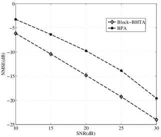
Fig. 1: NMSE (dB) versus SNR for Block-BHTA and BPA. The results are averaged over 400 trials.

We compare the Block-BHTA and BPA at different noise levels. In this experiment $N=192$ and $M=512$. We add the Gaussian white noise so that SNR, defined in (27), varies between 10 dB and 30 dB for each generated signal.

Figure 1 shows the NMSE (dB) versus SNR for both Block-BHTA and BPA. It is seen that Block-BHTA exhibit significant performance gain (almost 5 dB) over BPA.

In the second experiment, we examine the influence of the block size and the number of blocks on the estimation performance of the Block-BHTA where the block partition is unknown. Towards that end, we set up a simulation to compare the Block-BHTA with some recently developed algorithms for block sparse signal reconstruction, such as the block sparse Bayesian learning algorithm (BSBL) [11], the expanded block sparse Bayesian learning algorithm (EBSBL) [11], the cluster-structured MCMC algorithm (CluSS-MCMC) [9], and the pattern-coupled sparse Bayesian learning algorithm (PC-SBL) [12]. The size of matrix $\boldsymbol{\Phi}$ is $256\times 512$, $\mathrm{SNR}=15\mathrm{dB}$, and $\sigma_{\theta}=1$.

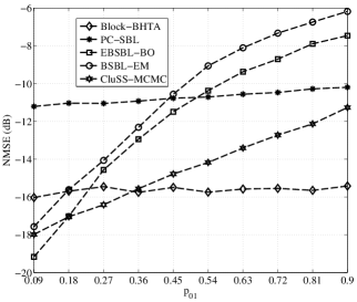
Fig. 2: NMSE versus $p_{01}$ for Block-BHTA and other algorithms. The results are averaged over 400 trials.

Recall from Section II that the block size and the number of blocks of $\mathbf{w}$ are proportional to $1/p_{01}$. That is, when $p_{01}$ is small $\mathbf{w}$ comprises small number of blocks with big sizes and vice versa. Hence, we vary the value of $p_{01}$ between $0.09$ and $0.9$ to obtain the NMSE (dB) for various algorithms. The results of NMSE (dB) versus $p_{01}$ is shown in Fig. 2. As seen from the figure, for $p_{01}\geq 0.36$ the Block-BHTA outperforms all other algorithms.

V Conclusion

This letter has presented a novel Block-BHTA to recover the block-sparse signals whose structure of block sparsity is completely unknown. The proposed Block-BHTA uses a Bayesian hypothesis testing to detect and recover the support of the block sparse signal. For amplitude recovery, Block-BHTA utilizes a linear MMSE to estimate the nonzero amplitudes of the detected supports. Simulation results demonstrate that Block-BHTA outperforms the BPA by almost 5 dB performance gain. The Block-BHTA also outperforms many state-of-the-art algorithms when the block-sparse signal comprises a large number of blocks with short lengths.

References

• [1] Y. C. Eldar, P. Kuppinger, and H. Bolcskei, “Block-sparse signals: Uncertainty relations and efficient recovery,” Signal Processing, IEEE Transactions on, vol. 58, no. 6, pp. 3042–3054, 2010.
• [2] Y. C. Eldar and M. Mishali, “Robust recovery of signals from a structured union of subspaces,” Information Theory, IEEE Transactions on, vol. 55, no. 11, pp. 5302–5316, 2009.
• [3] M. Yuan and Y. Lin, “Model selection and estimation in regression with grouped variables,” Journal of the Royal Statistical Society. Series B: Statistical Methodology, vol. 68, no. 1, pp. 49–67, 2006.
• [4] R. G. Baraniuk, V. Cevher, M. F. Duarte, and C. Hegde, “Model-based compressive sensing,” Information Theory, IEEE Transactions on, vol. 56, no. 4, pp. 1982–2001, 2010.
• [5] M. Mishali and Y. C. Eldar, “Blind multiband signal reconstruction: Compressed sensing for analog signals,” Signal Processing, IEEE Transactions on, vol. 57, no. 3, pp. 993–1009, 2009.
• [6] R. Gribonval and E. Bacry, “Harmonic decomposition of audio signals with matching pursuit,” Signal Processing, IEEE Transactions on, vol. 51, no. 1, pp. 101–111, 2003.
• [7] M. F. Duarte and Y. C. Eldar, “Structured compressed sensing: From theory to applications,” Signal Processing, IEEE Transactions on, vol. 59, no. 9, pp. 4053–4085, 2011.
• [8] Z. Zhilin and B. D. Rao, “Sparse signal recovery with temporally correlated source vectors using sparse bayesian learning,” Selected Topics in Signal Processing, IEEE Journal of, vol. 5, no. 5, pp. 912–926, 2011.
• [9] L. Yu, H. Sun, J. P. Barbot, and G. Zheng, “Bayesian compressive sensing for cluster structured sparse signals,” Signal Processing, vol. 92, no. 1, pp. 259–269, 2012.
• [10] T. Peleg, Y. C. Eldar, and M. Elad, “Exploiting statistical dependencies in sparse representations for signal recovery,” Signal Processing, IEEE Transactions on, vol. 60, no. 5, pp. 2286–2303, 2012.
• [11] Z. Zhang and B. D. Rao, “Extension of SBL algorithms for the recovery of block sparse signals with intra-block correlation,” Signal Processing, IEEE Transactions on, vol. 61, no. 8, pp. 2009–2015, 2013.
• [12] J. Fang, Y. Shen, H. Li, and P. Wang, “Pattern-coupled sparse bayesian learning for recovery of block-sparse signals,” Signal Processing, IEEE Transactions on, vol. 63, no. 2, pp. 360–372, 2015.
• [13] H. Zayyani, M. Babaie-Zadeh, and C. Jutten, “Bayesian pursuit algorithm for sparse representation,” in Acoustics, Speech and Signal Processing, 2009. ICASSP 2009. IEEE International Conference on, April 2009, pp. 1549–1552.
• [14] J. Kang, H.-N. Lee, and K. Kim, “Bayesian hypothesis test using nonparametric belief propagation for noisy sparse recovery,” Signal Processing, IEEE Transactions on, vol. 63, no. 4, pp. 935–948, 2015.
• [15] M. Zimmermann and K. Dostert, “Analysis and modeling of impulsive noise in broad-band powerline communications,” Electromagnetic Compatibility, IEEE Transactions on, vol. 44, no. 1, pp. 249–258, 2002.
• [16] J. Ziniel and P. Schniter, “Dynamic compressive sensing of time-varying signals via approximate message passing,” Signal Processing, IEEE Transactions on, vol. 61, no. 21, pp. 5270–5284, 2013.
• [17] H. Zayyani, M. Babaie-Zadeh, and C. Jutten, “An iterative bayesian algorithm for sparse component analysis in presence of noise,” Signal Processing, IEEE Transactions on, vol. 57, no. 11, pp. 4378–4390, 2009.
• [18] S. M. Kay, Fundamentals of Statistical Signal Processing Volume II: Estimation Theory.   New Jersey, U.S.A: Englewood Cliffs, 1993.
• [19] M. Korki, J. Zhang, C. Zhang, and H. Zayyani, “An iterative bayesian algorithm for block-sparse signal reconstruction,” in Acoustics, Speech and Signal Processing (ICASSP), 2015 IEEE International Conference on.