A quaternion-based model for optimal control of the SkySails airborne wind energy system

Abstract.

Airborne wind energy systems are capable of extracting energy from higher wind speeds at higher altitudes. The configuration considered in this paper is based on a tethered kite flown in a pumping orbit. This pumping cycle generates energy by winching out at high tether forces and driving a generator while flying figures-of-eight, or lemniscates, as crosswind pattern. Then, the tether is reeled in while keeping the kite at a neutral position, thus leaving a net amount of generated energy. In order to achieve an economic operation, optimization of pumping cycles is of great interest.

In this paper, first the principles of airborne wind energy will be briefly revisited. The first contribution is a singularity-free model for the tethered kite dynamics in quaternion representation, where the model is derived from first principles. The second contribution is an optimal control formulation and numerical results for complete pumping cycles. Based on the developed model, the setup of the optimal control problem (OCP) is described in detail along with its numerical solution based on the direct multiple shooting method in the CasADi optimization environment. Optimization results for a pumping cycle consisting of six lemniscates show that the approach is capable to find an optimal orbit in a few minutes of computation time. For this optimal orbit, the power output is increased by a factor of two compared to a sophisticated initial guess for the considered test scenario.

1. Introduction

The idea of airborne wind energy (AWE) is to generate usable power by airborne devices. In contrast to towered wind turbines, airborne wind energy systems are flying, usually connected by a tether to the ground, like kites or tethered balloons. AWE systems exploit the relative velocity between the airmass and the ground and maintain a tension in the tether. They can be connected to a stationary ground station, or to another moving, but non-flying object, like a land or sea vehicle. Power is generated in form of a traction force, e.g. to a moving vehicle, or in form of electricity. The three major reasons why people are interested in airborne wind energy for electricity production are the following:

• First, like solar, wind power is one of the few renewable energy resources that is in principle large enough to satisfy all of humanity’s energy needs.

• Second, in contrast to ground-based wind turbines, airborne wind energy devices might be able to reach higher altitudes, tapping into a large and so far unused wind power resource [5]. The winds in higher altitudes are typically stronger and more consistent than those close to the ground, both on- and off-shore.

• Third, and most important, airborne wind energy systems might need less material investment per unit of usable power than most other renewable energy sources. This high power-to-mass ratio promises to make large scale deployment of the technology possible at comparably low costs.

In order to achieve an economic and competitive operation of airborne wind energy (AWE) setups, optimal control of energy production is the key to success. In this paper, a novel formulation of the dynamics of a specific AWE system is given, and it is shown how it allows one to solve challenging optimal control problems for this system.

The paper is organized as follows: in Section 2, we introduce the main ideas of airborne wind energy, following the lines of [8], and then explain in Section 3 the experimental system developed by the company SkySails, the modeling of which is the main subject of this paper. Starting point is an existing differential equation model of the system from [9], described in Section 4, which suffers from singularities caused by the choice of coordinate system. The main contribution of this paper is presented in Section 5, where a new singularity free model based on quaternions is developed. It is demonstrated by numerical simulation that the old and new model describe identical system dynamics when away from the singularities, while only the new model can be reliably simulated everywhere. It is then shown in Section 6 how the new quaternion-based model can be used to formulate the complex periodic optimal control problem (OCP). In Sect. 7, the discrete formulation of the OCP to be solved in the dynamic optimization environment CasADi [4] is given. Furthermore, resulting complete operational pumping cycles for the SkySails airborne wind energy system are presented. The paper ends with a conclusion in Section 8.

2. Crosswind kite power and pumping cycles

Every hobby kite pilot or kite surfer knows this observation: As soon as a kite is flying fast loops in a crosswind direction the tension in the lines increases significantly. The hobby kite pilots have to compensate the tension strongly with their hands while kite surfers make use of the enormous crosswind power to achieve high speeds and perform spectacular stunts. The reason for this observation is that the aerodynamic lift force ${F_{\mathrm{L}}}$ of an airfoil increases with the square of the flight velocity, or more exactly, with the apparent airspeed at the wing, which we denote by ${v_{\mathrm{a}}}$. More specifically,

$${F_{\mathrm{L}}}=\frac{1}{2}\rho A{C_{\mathrm{L}}}{v^{2}_{{\mathrm{a}}}},$$ (1)

where $\rho$ is the density of the air, $A$ the airfoil area, and ${C_{\mathrm{L}}}$ the lift coefficient which depends on the geometry of the airfoil.

Thus, if we fly a kite in crosswind direction with a velocity ${v_{\mathrm{a}}}$ that is ten times faster than the wind speed ${v_{\mathrm{w}}}$, the tension in the line will increase by a factor of hundred in comparison to a kite that is kept at a static position in the sky. The key observation is now that the high speed of the kite can be maintained by the ambient wind flow, and that either the high speed itself or the tether tension can be made useful for harvesting a part of the enormous amount of power that the moving wing can potentially extract from the wind field.

The idea of power generation with tethered airfoils flying fast in a crosswind direction was already in the 1970’s and 1980’s investigated in detail by the American engineer Miles Loyd [19]. He was arguably the first to compute the power generation potential of fast flying tethered wings - a principle that he termed crosswind kite power. Loyd investigated (and also patented) the following idea: an airplane, or kite, is flying on circular trajectories in the sky while being connected to the ground with a strong tether. He described two different ways to make this highly concentrated form of wind power useful for human needs, that he termed lift mode and drag mode: while the lift mode uses the tension in the line to pull a load on the ground, the drag mode uses the high apparent airspeed to drive a small wind turbine on the wing.

This paper is concerned with systems operating in lift mode, which has the advantage over the drag mode that that it does not need high voltage electrical power transmission via the tether. The idea is to directly use the strong tether tension to unroll the tether from a drum, and the rotating drum drives an electric generator. As both the drum and generator can be placed on the ground, we call this concept also ground-based generation or traction power generation. For continuous operation, one has to periodically retract the tether. One does so by changing the flight pattern to one that produces much less lifting force. This allows one to reel in the tether with a much lower energy investment than what was gained in the power production phase. The power production phase is also called reel-out phase, and the retraction phase reel-in or return phase. Loyd coined the term lift mode because one uses mainly the lifting force of the wing. But due to the periodic reel-in and reel-out motion of the tether, this way of ground-based power generation is often also called pumping mode; sometimes even the term Yo-Yo mode was used to describe it.

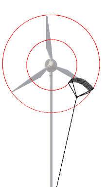
Figure 1. The basic idea of the power generating device is to only build the wing tips of a gigantic windmill, in form of tethered airfoils, i.e. kites. Fast crosswind motion of the kites creates an enormous traction force [graphics courtesy Boris Houska].

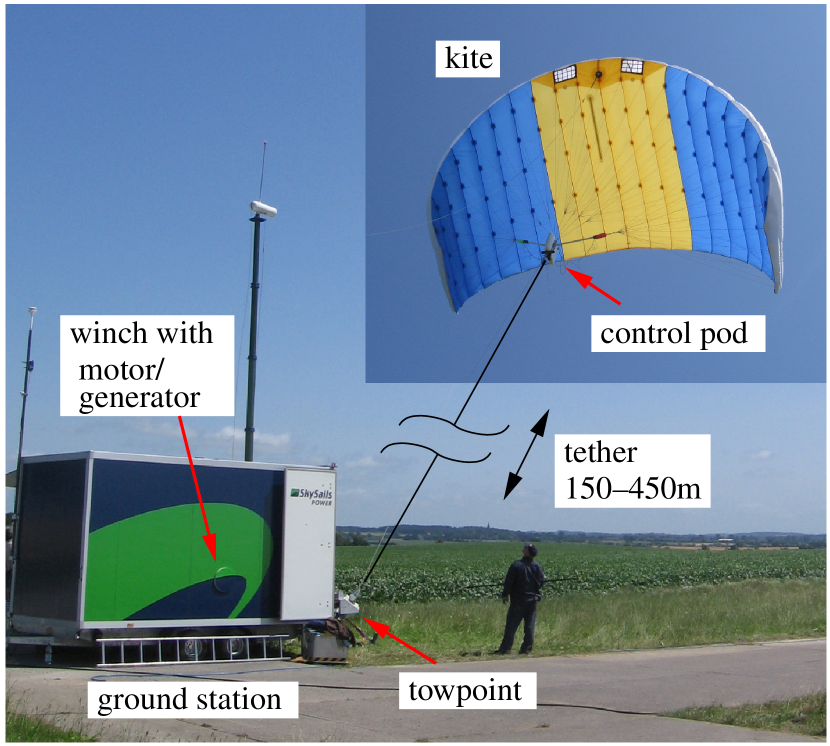
Figure 2. SkySails functional prototype setup for kites of sizes ranging from 20 to 40 m² (30 m² shown here). A tether in the range 150–400 m transfers the forces from the flying system to the ground based main winch, which is attached to a motor/generator. A specific feature of this setup is the single tether and the airborne control pod located under the kite. The steering actuator in the control pod pulls certain lines in order to steer the kite.

It is interesting to compare crosswind kite power systems with a conventional wind turbine, as done in Fig. 2, which shows a conventional wind turbine superposed with an airborne wind energy system. Seen from this perspective, the idea of AWE is to only build the fastest moving part of a large wind turbine, the tips of the rotor blades, and to replace them by automatically controlled fast flying tethered kites. The motivation for this is the fact that the outer 30% of the blades of a conventional wind turbine provide more than half of the total power, while they are much thinner and lighter than the inner parts of the blades. Roughly speaking, the idea of airborne wind energy systems is to replace the inner parts of the blades, as well as the tower, by a tether.

The power $P$ that can be generated with a tethered airfoil operated either in drag or in lift mode had under idealized assumptions been estimated by Loyd [19] to be approximately given by

$$P=\frac{2}{27}\rho A{v^{3}_{{\mathrm{w}}}}{C_{\mathrm{L}}}\left(\frac{{C_{\mathrm{L}}}}{{C_{\mathrm{D}}}}\right)^{2},$$ (2)

where $A$ is the area of the wing, ${C_{\mathrm{L}}}$ the lift and ${C_{\mathrm{D}}}$ the drag coefficients, and ${v_{\mathrm{w}}}$ the wind speed. Note that the lift-to-drag ratio $E\doteq\frac{{C_{\mathrm{L}}}}{{C_{\mathrm{D}}}}$ enters the formula quadratically and is thus an important wing property for crosswind AWE systems. For airplanes, this ratio is also referred to as the gliding number; it describes how much faster a glider without propulsion can move horizontally compared to its vertical sink rate.

Since the first proposal of using tethered wings for energy harvesting by Loyd, academic research and industrial development activities in the field of airborne wind energy (AWE) have been significantly increasing, especially during the last 10 years. The main advantage of the AWE technology is that airborne systems are capable of harvesting energy from higher wind speeds at higher altitudes. In addition, as most setups require less installation efforts compared to conventional wind turbines, e.g. foundations and towers, this technology is a promising candidate to become an additional source of renewable energy in the near future. For an overview on the different geometries which have been developed so far, the reader is referred to [13] and the monograph on AWE [2].

3. The SkySails Power prototype

The geometry under consideration in this paper is based on the SkySails Power prototype, shown in Fig. 2. This setup features an airborne control pod located under the soft kite connected to a ground based winch with motor/generator by a single tether. The functional prototype successfully demonstrated fully automated energy generation by autonomously controlled pumping cycles [12]. Trajectory of an experimentally flown pumping cycle [12]. The principle of energy generation is depicted in Fig. 3 and shall be briefly summarized: during the power phase, the kite is flown dynamically in lemniscates (figures of eight). This dynamical crosswind flight leads to high tether forces. By reeling out the tether, electrical energy is produced. At a certain line length, the kite is transferred to the neutral zenith position. At this low-force position, the tether is reeled in (return phase) consuming a certain portion of the previously generated energy. Finally, a reasonable amount of generated net power remains. Hence, the average power output over complete cycles will be the target of the optimization implementation presented in this paper.

The optimal control is based on a dynamical model of the system, and the chosen numerical techniques are similar to the ones used in [16]. In order to allow for optimization of complete pumping cycles, a simple model should be chosen in order to keep the number of optimization variables low. The model developed in this paper is based on a very simple model set up for the SkySails system [9], which describes the basic dynamic properties of the system and has been experimentally validated [11]. The quaternion representation allows for singularity-free equations of motion, and the replacement of trigonometric functions seems to be advantageous for the optimization process.

A further advantage of the considered system is that an experimentally flown trajectory (see e.g. Fig. 3) can be used as initial guess and the optimization result can be directly compared to it in return. It should be noted that the optimization has to be subject to certain geometrical constraints, which will be discussed in this paper. Particularly, topological constraints have to be imposed to preserve the topology of the pumping cycle during the optimization process (the 6 lemniscates given in the initial guess, compare Fig. 3).

4. Setup and reference kite model

In this section, the model from [9], [11] is briefly summarized. The coordinate system is defined in Fig. 3.

Figure 3. Coordinate system definitions of the fixed reference vectors ${\bf e}_{x},{\bf e}_{y},{\bf e}_{z}$ and the body frame vectors ${\bf e}_{\rm roll}$, ${\bf e}_{\rm pitch}$ and ${\bf e}_{\rm yaw}$. The position is determined by the two angles $\varphi$, $\vartheta$ and the tether length $l$. The wind direction is defined in ${\bf e}_{x}$-direction.

The state vector of the dynamical system consists of the 3-dimensional orientation of the flying system, given by $\left\{\psi,\varphi,\vartheta\right\}$ and the tether length $l$.

$${\bf x}=\left[\psi,\varphi,\vartheta,l\right]^{\top}$$ (3)

Note that the tether of the system leads to a relation between orientation and position, which is given in the basis $\{{\bf e}_{x},{\bf e}_{y},{\bf e}_{z}\}$ by:

$${\bf r}=l\left[\begin{array}[]{c}\cos\vartheta\\ \sin\varphi\sin\vartheta\\ -\cos\varphi\sin\vartheta\end{array}\right]$$ (4)

The wind direction is defined in ${\bf e}_{x}$-direction. In order to provide a clear picture of the coordinate system definition, a comparison with the navigation task on earth shall be discussed as illustrated in Fig. 5.

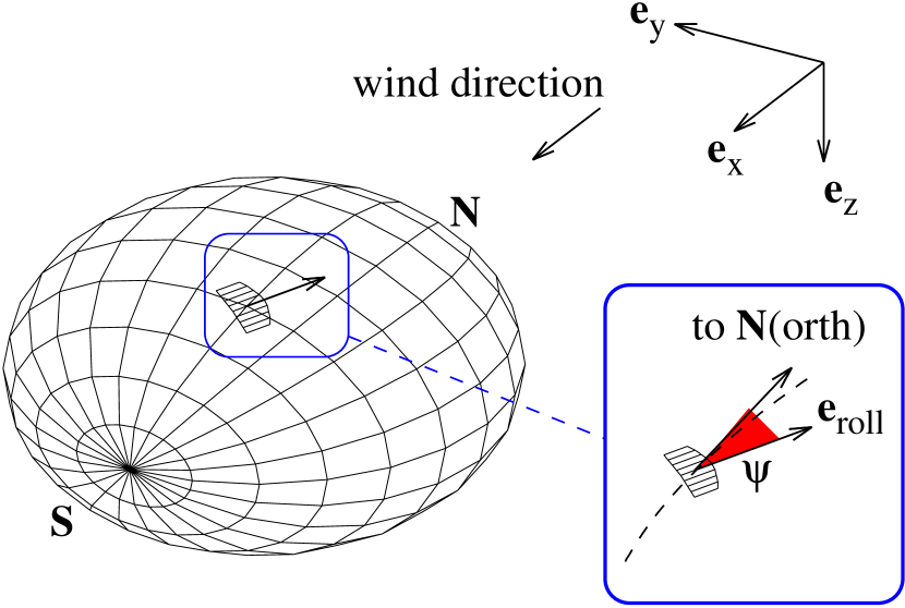
Figure 4. Demonstrative explanation of the used Euler angles by comparing them to angles used for navigation on earth. For that purpose, the earth’s rotation axis has to be tilted by 90 degrees with the north pole towards the wind direction. The angles $\varphi$, $\vartheta$ correspond to the position on earth and $\psi$ to the bearing. The exact mapping is given in Table 5.

table angle in model ’earth’ navigation quantity $\varphi$ earth longitude $\vartheta$ earth latitude $\psi$ bearing (direction w.r.t. north pole)

Figure 5. Mapping of the Euler angles of the tethered system to earth navigation quantities (compare Fig. 5).

The coordinate system corresponds to an earth coordinate system with symmetry (rotational) axis in wind direction, which could be achieved by rotating the north pole by 90 degrees towards the wind direction. According to the angle mapping given in Table 5, the two angles $\varphi,\vartheta$ correspond to longitude and latitude, hence determine the position on earth. The orientation angle $\psi$ corresponds to bearing, i.e. direction w.r.t. north in our earth system. This angle determines the direction of motion (course) and the angle of $\psi=0$ describes heading directly against the wind. It should be finally noted that due to the ambient wind, the angle $\psi$ does not exactly coincide the kinematic flight direction (course). This effect is fully covered by the developed model and further explained in [12].

The input vector of the model comprises the inputs of the two control actuators: the steering deflection of the airborne control pod, $\delta$ and the winch speed of the tether $v^{\rm(winch)}$, respectively.

$${\bf u}=\left[\delta,v^{\rm(winch)}\right]^{\top}$$ (5)

In the following, the equations of motion shall be summarized for reference purpose only. This model was derived based on the same assumptions as those that will be used in the subsequent section for the derivation of the quaternion representation. As conducted in detail in [9], [11], the equations of motion read:

$$\dot{\psi} = g_{\rm k}\,v_{\rm a}\,\delta+\dot{\varphi}\cos\vartheta$$ (6)

$$\dot{\varphi} = -\frac{v_{\rm a}}{l\sin\vartheta}\sin\psi$$ (7)

$$\dot{\vartheta} = -\frac{v_{\rm w}}{l}\sin\vartheta+\frac{v_{\rm a}}{l}\cos\psi$$ (8)

$$\dot{l} = v^{\rm(winch)}$$ (9)

Here, the airpath speed of the kite, $v_{\rm a}$, is given by

$$v_{\rm a}=v_{\rm w}E\cos\vartheta-\dot{l}E.$$ (10)

The set of equations involves three parameters: lift-to-drag (glide) ratio $E$, steering response proportionality constant $g_{\rm k}$ and ambient wind speed $v_{\rm w}$. Further explanations of parameters including values used later in the paper are summarized in Table 10. Description of system parameters and values used for optimization symbol value description $A$ 21.0 m² projected area of the kite $C_{\rm R}$ 1.0 aerodynamic force coefficient, given by $C_{\rm D}=\sqrt{C_{\rm L}^{2}+C_{\rm D}^{2}}$ for aerodynamic lift (drag) coefficient $C_{\rm L}$ ($C_{\rm D}$) $\dot{\delta}_{\rm max}$ 0.6 1/s maximal control actuator steering speed $\delta_{\rm max}$ 0.7 maximal control actuator steering deflection $E$ 5.0 lift-to-drag (glide) ratio. Note, that in contrast to most other systems, the SkySails system is operated at constant glide ratio $g_{\rm k}$ 0.1 rad/m proportionality constant relating turn rate of the kite to steering actuator deflection $l_{\rm max}$ 300 m maximal available tether length $\theta_{\rm min}$ 0.35 rad minimal elevation angle w.r.t. the horizontal plane $\varrho$ 1.2 kg/m³ air density $v_{\rm a,min}$ 5.0 m/s minimal air path speed in order to guarantee flight stability and keep system tethered (this corresponds to free flight velocity) $v^{\rm(winch)}_{\rm min}$ $-5.0$ m/s typically chosen as $-v_{\rm w}/2$, leads to a windward limit of $\approx 110^{\circ}$ $v_{\rm w}$ 10 m/s ambient wind speed Finally, the tether force can be computed based on the air path speed $v_{\rm a}$ by

$$F_{\rm tether}=\frac{\varrho AC_{\rm R}}{2}\frac{E}{\sqrt{1+E^{2}}}v_{\rm a}^{2}$$ (11)

with density of air $\varrho$, projected kite area $A$ and aerodynamic force coefficient $C_{\rm R}$.

5. Quaternion based kite model

In the following, the equations of motion shall be derived in a singularity-free formulation based on quaternions. Quaternions are a well-known tool in aerospace modeling and estimation to avoid the singularities of Euler angles [18]. An alternative singularity-free representation could be based on rotation matrices as natural coordinates directly, as is shown for modeling of AWE systems in [15]. Note that the rotation matrix in the following will be used only as intermediate step in the derivation towards quaternions. The base coordinate system is depicted in Fig. 5a. The time dependence w.r.t. to this reference frame is expressed by rotation matrices $R(t)\in\mathrm{SO}(3)$, i.e.

$${\bf e}_{\rm roll}(t) = -R(t){\bf e}_{z}$$ (12)

$${\bf e}_{\rm pitch}(t) = -R(t){\bf e}_{y}$$ (13)

$${\bf e}_{\rm yaw}(t) = -R(t){\bf e}_{x}$$ (14)

The zero-rotation state is defined by $R\doteq I$, corresponding to ${\bf e}_{\rm yaw}=-{\bf e}_{x}$, ${\bf e}_{\rm pitch}=-{\bf e}_{y}$ and ${\bf e}_{\rm roll}=-{\bf e}_{z}$ as illustrated in Fig. 6.

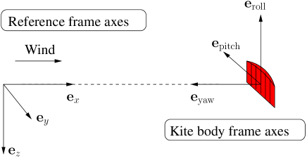
Figure 6. Reference frame axes for the derivation of the quaternion equations of motion. The depicted orientation corresponds to the zero-rotation, i.e. $R=I$ or ${\bf q}=[1,0,0,0]$.

Note that this seems to be an arbitrary choice a priori. However defining the ambient wind direction, given by ${\bf e}_{x}$, in the kite’s yaw-axis leads to a beneficial simplicity of the equations of motion later.

It should be emphasized that due to the nature of the tethering, position and orientation are related. Hence, the position of the kite is given by

$${\bf r}(t)=-l(t){\bf e}_{\rm yaw}(t)=l(t)R(t){\bf e}_{x}$$ (15)

The air path speed vector can be calculated as sum of the ambient wind vector $v_{\rm w}{\bf e}_{x}$ and reversed kinematic velocity vector $-\dot{{\bf r}}$ (apparent wind opposed to motion). Using the time derivative of (15) and introducing the speeds $v_{\rm roll}$ and $v_{\rm pitch}$ in the tangent plane, compare Fig. 7, yields

$${\bf v}_{\rm a}(t)=v_{\rm w}{\bf e}_{x}-v_{\rm pitch}(t){\bf e}_{\rm pitch}(t)-v_{\rm roll}(t){\bf e}_{\rm roll}(t)+\dot{l}(t){\bf e}_{\rm yaw}(t)$$ (16)

5.1. Model assumptions

For AWE systems, the aerodynamic forces are typically large compared to masses, which in fact is a prerequisite for tethered flight. This is particularly true for the SkySails Power system. Therefore, acceleration effects play a minor role and can be neglected. In addition, the system is assumed to fly always in its aerodynamic equilibrium state. These two simplifications lead to the simple structure of the equations of motion.

5.1.1. Aerodynamics

Figure 7. The kite is assumed to always fly in an aerodynamic equilibrium state. As aerodynamic model, absence of transversal air flow (top view) and constant lift-to-drag-ratio (side view) is demanded. Figure taken from [11]

The aerodynamics of the system is reduced to two conditions, depicted in Fig. 7 and given in the following.

1. The kite experiences no transversal wind flow, i.e. no ’side-slip’ angle occurs, compare Fig. 7b.

   $$\left\langle{\bf e}_{\rm pitch}(t),{\bf v}_{\rm a}(t)\right\rangle=0$$ (17)

   Inserting (16) yields

   $$\left\langle{\bf e}_{\rm pitch}(t),v_{\rm w}{\bf e}_{x}\right\rangle-v_{\rm pitch}(t)+\dot{l}\underbrace{\left\langle{\bf e}_{\rm pitch}(t),{\bf e}_{\rm yaw}(t)\right\rangle}_{=0}=0$$ (18)

   Thus, the condition results in

   $$v_{\rm pitch}(t)=-v_{\rm w}\left\langle R(t){\bf e}_{y},{\bf e}_{x}\right\rangle$$ (19)

2. The lift-to-drag ratio is constant and given by the parameter $E$. Hence, the kite is assumed to fly always at the same angle of attack. Considering the geometry of Fig. 7c) yields

   $$\left\langle{\bf e}_{\rm roll}(t),{\bf v}_{\rm a}(t)\right\rangle=E\left\langle{\bf e}_{\rm yaw}(t),{\bf v}_{\rm a}(t)\right\rangle$$ (20)

   Inserting (16) produces

   $$v_{\rm roll}(t)=v_{\rm w}\left\langle R(t)(E{\bf e}_{x}-{\bf e}_{z}),{\bf e}_{x}\right\rangle-E\dot{l}(t)$$ (21)

Finally, by considering the motion in the tangent plane, compare Fig. 7, the following relations for the turn rates in kite-body-frame can be derived. Motion in the tangent plane. Due to the tether, the velocities in the tangent plane $v_{\rm roll}$ and $v_{\rm pitch}$ determine $\omega_{\rm roll}$ and $\omega_{\rm pitch}$ as given in (22) and (23).

$$\omega_{\rm roll} = \frac{v_{\rm pitch}(t)}{l(t)}=-\frac{v_{\rm w}}{l(t)}\left\langle R(t){\bf e}_{y},{\bf e}_{x}\right\rangle$$ (22)

$$\omega_{\rm pitch} = -\frac{v_{\rm roll}(t)}{l(t)}=-\frac{v_{\rm w}}{l(t)}\left\langle R(t)(E{\bf e}_{x}-{\bf e}_{z}),{\bf e}_{x}\right\rangle+E\frac{\dot{l}(t)}{l(t)}$$ (23)

5.1.2. Steering

Steering of the kite is accomplished by the control actuator in the control pod. Applying an actuator deflection $\delta$ to the steering lines tilts the kite canopy resulting in a curve flight or turn rate around the ${\bf e}_{\rm yaw}$-axis. The steering behavior can be described by the following equation

$$\omega_{\rm yaw}=g_{\rm k}v_{\rm a}\delta$$ (24)

This turn-rate law states that the rotation rate is proportional to a constant system parameter $g_{\rm k}$, the deflection $\delta$ and the scalar air path speed $v_{\rm a}$, which is defined as component of ${\bf v}_{\rm a}$ in $-{\bf e}_{\rm roll}$-direction

$$v_{\rm a}\doteq-\left\langle{\bf e}_{\rm roll}(t),{\bf v}_{\rm a}(t)\right\rangle=\left\langle R(t){\bf e}_{z},{\bf v}_{\rm a}(t)\right\rangle$$ (25)

The validity of the turn-rate law has been experimentally shown for different kites [9], [14], [17]. In addition, a nice derivation based on geometric considerations can be found in [14]. It should be mentioned that correction terms for mass effects [10] and aerodynamic effects [7] might be added, but are neglected in this paper.

5.2. Quaternions

The final formulation of the equations of motion is based on quaternions [18], introduced as

$${\bf q}=\left[\begin{array}[]{c}q_{0}\\ q_{1}\\ q_{2}\\ q_{3}\end{array}\right]$$ (26)

The time evolution as function of turn rates, which are given in the body frame, reads

$$\dot{{\bf q}}=\frac{1}{2}\left[\begin{array}[]{cccc}0&-\omega_{x}&-\omega_{y}&-\omega_{z}\\ \omega_{x}&0&\omega_{z}&-\omega_{y}\\ \omega_{y}&-\omega_{z}&0&\omega_{x}\\ \omega_{z}&\omega_{y}&-\omega_{x}&0\end{array}\right]{\bf q}$$ (27)

Mapping of the kite axes to $\omega_{x},\omega_{y},\omega_{z}$ has to be considered for $R\!=\!I$. Regarding (12–14) or Fig. 6 yields $\omega_{x}\!=\!-\omega_{\rm yaw}$, $\omega_{y}\!=\!-\omega_{\rm pitch}$ and $\omega_{z}\!=\!-\omega_{\rm roll}$. The quaternion time evolution then results in

$$\dot{{\bf q}}=\frac{1}{2}\left[\begin{array}[]{cccc}0&\omega_{\rm yaw}&\omega_{\rm pitch}&\omega_{\rm roll}\\ -\omega_{\rm yaw}&0&-\omega_{\rm roll}&\omega_{\rm pitch}\\ -\omega_{\rm pitch}&\omega_{\rm roll}&0&-\omega_{\rm yaw}\\ -\omega_{\rm roll}&-\omega_{\rm pitch}&\omega_{\rm yaw}&0\end{array}\right]{\bf q}$$ (28)

The relation to the rotation can be given by

$$R(t)=\left[\begin{array}[]{ccc}q_{0}^{2}+q_{1}^{2}-q_{2}^{2}-q_{3}^{2}&2(q_{1}q_{2}-q_{0}q_{3})&2(q_{1}q_{3}+q_{0}q_{2})\\[8.0pt] 2(q_{1}q_{2}+q_{0}q_{3})&q_{0}^{2}-q_{1}^{2}+q_{2}^{2}-q_{3}^{2}&2(q_{2}q_{3}-q_{0}q_{1})\\[8.0pt] 2(q_{1}q_{3}-q_{0}q_{2})&2(q_{2}q_{3}+q_{0}q_{1})&q_{0}^{2}-q_{1}^{2}-q_{2}^{2}+q_{3}^{2}\end{array}\right]$$ (29)

The derivation of the system’s equations of motion is done as follows: The turn rates in kite-body-frame, $\omega_{\rm roll}$, $\omega_{\rm pitch}$ and $\omega_{\rm yaw}$ are expressed as functions of ${\bf q}$ and subsequently inserted in (28). In order to achieve this, (29) is used for $R(t)$ and inserted into (22), (23) and (24).

5.3. Equations of motion

The state vector for the quaternion formulation is given by

$$\left[q_{0},q_{1},q_{2},q_{3},l\right]^{\top}$$ (30)

and the input vector by

$$\left[\delta,v^{\rm(winch)}\right]^{\top}$$ (31)

Performing the derivation steps of the previous section yields the following set of equations of motion:

$$\dot{{\bf q}} = \frac{v_{\rm a}}{2l}\left[\begin{array}[]{c}-q_{2}\\ -q_{3}\\ q_{0}\\ q_{1}\end{array}\right]+\frac{v_{\rm w}}{l}\left[\begin{array}[]{c}q_{0}(q_{2}^{2}+q_{3}^{2})\\ q_{1}(q_{2}^{2}+q_{3}^{2})\\ -q_{2}(q_{0}^{2}+q_{1}^{2})\\ -q_{3}(q_{0}^{2}+q_{1}^{2})\end{array}\right]+\frac{g_{\rm k}v_{\rm a}\delta}{2}\left[\begin{array}[]{c}q_{1}\\ -q_{0}\\ -q_{3}\\ q_{2}\end{array}\right]$$ (44)

$$\dot{l} = v^{\rm(winch)}$$ (45)

with air path speed

$$v_{\rm a}=Ev_{\rm w}(q_{0}^{2}+q_{1}^{2}-q_{2}^{2}-q_{3}^{2})-E\dot{l}$$ (46)

It should be remarked that if the winch speed is defined relative to the wind speed by substituting $\dot{l}=v_{\rm w}v^{\rm winch}_{\rm rel}$, the product of wind speed $v_{\rm w}$ and time $t$ (or cycle time $T$) becomes an invariant. As a consequence, solutions for different wind speeds are simply obtained by scaling the dynamic’s time axis proportional to $1/v_{\rm w}$.

Although these equations of motion (EQM) preserve the quaternion norm $(\mathrm{d}/\mathrm{d}t)\|{\bf q}(t)\|=0$, a stabilization term in order to compensate for numerical inaccuracies should be added. The EQM for the numerical optimization read then

$$\dot{{\bf q}}=\Phi(\cdot)-\gamma_{q}(\|{\bf q}\|^{2}-1){\bf q}$$ (47)

where $\Phi(\cdot)$ denotes the equations of motion (44–46) and the damping constant $\gamma_{q}$ is chosen to lead to a slow decay ($\gamma_{q}=0.01$ 1/s for the parameters given in Table 10).

5.4. Transformation to Euler angles for comparison

For sake of completeness and in order to allow for a simple geometric interpretation of the results in the Cartesian coordinate system (see Fig. 5), transformations from the set of Euler angles $\{\varphi,\vartheta,\psi\}$ to quaternions and back shall be summarized. The sequence of rotations

$$R=R_{x}(\varphi)R_{y}(\vartheta)R_{x}(-\psi)$$ (48)

is considered in quaternion representation

$${\bf q} = \left[\begin{array}[]{c}\cos\left(\frac{\varphi}{2}\right)\\ \sin\left(\frac{\varphi}{2}\right)\\ 0\\ 0\end{array}\right]\otimes\left[\begin{array}[]{c}\cos\left(\frac{\vartheta}{2}\right)\\ 0\\ \sin\left(\frac{\vartheta}{2}\right)\\ 0\end{array}\right]\otimes\left[\begin{array}[]{c}\cos\left(\frac{\psi}{2}\right)\\ -\sin\left(\frac{\psi}{2}\right)\\ 0\\ 0\end{array}\right]$$ (61)

Calculating the quaternion product ($\otimes$) [18] of the single rotations yields

$${\bf q} = \left[\begin{array}[]{c}\cos\left(\frac{\varphi}{2}\right)\cos\left(\frac{\vartheta}{2}\right)\cos\left(\frac{\psi}{2}\right)+\sin\left(\frac{\varphi}{2}\right)\cos\left(\frac{\vartheta}{2}\right)\sin\left(\frac{\psi}{2}\right)\\ \sin\left(\frac{\varphi}{2}\right)\cos\left(\frac{\vartheta}{2}\right)\cos\left(\frac{\psi}{2}\right)-\cos\left(\frac{\varphi}{2}\right)\cos\left(\frac{\vartheta}{2}\right)\sin\left(\frac{\psi}{2}\right)\\ -\sin\left(\frac{\varphi}{2}\right)\sin\left(\frac{\vartheta}{2}\right)\sin\left(\frac{\psi}{2}\right)+\cos\left(\frac{\varphi}{2}\right)\sin\left(\frac{\vartheta}{2}\right)\cos\left(\frac{\psi}{2}\right)\\ \sin\left(\frac{\varphi}{2}\right)\sin\left(\frac{\vartheta}{2}\right)\cos\left(\frac{\psi}{2}\right)+\cos\left(\frac{\varphi}{2}\right)\sin\left(\frac{\vartheta}{2}\right)\sin\left(\frac{\psi}{2}\right)\end{array}\right]$$ (66)

The kite position w.r.t. $\{{\bf e}_{x},{\bf e}_{y},{\bf e}_{z}\}$ can be found by inserting (29) into (15) as

$${\bf r}=l\left[\begin{array}[]{c}(q_{0}^{2}+q_{1}^{2}-q_{2}^{2}-q_{3}^{2})\\ 2(q_{0}q_{3}+q_{1}q_{2})\\ 2(q_{1}q_{3}-q_{0}q_{2})\end{array}\right]$$ (67)

The Euler angles can be computed from the quaternions by

$$\varphi = \mathrm{atan2}\left((q_{0}q_{3}+q_{1}q_{2}),(q_{0}q_{2}-q_{1}q_{3})\right)$$ (68)

$$\vartheta = \arccos(q_{0}^{2}+q_{1}^{2}-q_{2}^{2}-q_{3}^{2})$$ (69)

$$\psi = \mathrm{atan2}\left((q_{0}q_{3}-q_{1}q_{2}),(q_{0}q_{2}+q_{1}q_{3})\right)$$ (70)

where $\mathrm{atan2}$ is the four-quadrant arctangent function.

5.5. Simulation example

In order to complete the presentation of the quaternion-based model, a simulation example will be discussed. The simulations have been carried out using the quaternion-based model on the one and the reference model from Sect. 4 on the other hand. Both computations have employed a Runge-Kutta-4 ODE propagation using timesteps of $\tau\!=\!0.1$ s, a tether length of $l\!=\!100$ m and the initial conditions $\varphi(0)\!=\!0,\vartheta(0)\!=\!\arctan(E)$ and $\psi(0)=0$. A constant steering command of $\delta\!=\!0.186$ has been used to fly next to the singularity of the Euler angle representation. Simulation of the simple model ODE, formulated in Euler angles (solid red) and quaternions (dashed blue). The 3d trajectory is shown on the left, the right plot zooms into the vicinity of the singularity, where the Euler angle formulation fails. The points in the right subfigure represent the discrete simulation timesteps of constant duration. The simulation results are depicted in Fig. 5.5. It can be recognized that the propagation of the model (6–10) fails due to the singularity, while the quaternion formulation (44–46) leads to correct numerical simulation results.

6. Optimal control problem formulation

The optimization task is to control power cycles with optimal power output averaged over complete cycles. This quantity is computed as integral over the mechanical power

$$\bar{P}=\frac{1}{T}\int\limits_{0}^{T}\dot{l}\,F_{\rm tether}\;\mathrm{d}t=\frac{\varrho AC_{\rm R}}{2}\frac{E}{\sqrt{1\!+\!E^{2}}}\frac{1}{T}\int\limits_{0}^{T}\dot{l}\,v_{\rm a}^{2}\;\mathrm{d}t$$ (71)

It should be mentioned at this point that an open loop optimal control problem is set up, which is based on controls as model input, but does not involve any feedback control based on measured values.

6.1. Setup of the optimization problem

As steering speed will also be limited, the steering deflection $\delta$ is introduced as additional state to the model and the pod steering actuator speed, defined as $\dot{\delta}_{\rm s}$, is used as control, instead. Further, the state $W$ with $W(0)=0$ for computing the integral in (71) is added. Thus, the following relations have to be added to complete the set of EQM (44–46)

$$\dot{\delta} = \dot{\delta}_{\rm s}$$ (72)

$$\dot{W} = \dot{l}v_{\rm a}^{2}$$ (73)

The control vector now reads

$${\bf u}=\left[\dot{\delta}_{\rm s},v^{\rm(winch)}\right]^{\top}$$ (74)

and the state

$${\bf x}=\left[W,\delta,l,q_{0},q_{1},q_{2},q_{3}\right]^{\top}$$ (75)

The NLP problem is formulated as minimization of

$$f=-\frac{1}{T}\int\limits_{0}^{T}\dot{l}v_{\rm a}^{2}\;\mathrm{d}t+\epsilon_{\delta}\int\limits_{0}^{T}|\dot{\delta}(t)|^{2}\;\mathrm{d}t=-\frac{W(T)}{T}+\epsilon_{\delta}\int\limits_{0}^{T}|\dot{\delta}(t)|^{2}\;\mathrm{d}t$$ (76)

The second term introduces a penalty in order to achieve a smooth steering behavior. The weighting factor $\epsilon_{\delta}$ has to be chosen appropriately.

The optimization, i.e. minimization of $f$, has to be carried out by variation of ${\bf x}(t),{\bf u}(t),T$ subject to the following constraints. First the optimization is subject to the model equations of motion (44–46). In addition, physical, geometrical and topological constraints have to be added, which will be discussed in the subsequent sections.

6.2. Physical constraints

Due to weight and geometrical design considerations for the airborne system, the two limitations of limited steering speed and deflection of the control pod actuator have to be taken into account. Hence, the steering speed limit is given by

$$|\dot{\delta}_{\rm s}|\leq\dot{\delta}_{\rm max}$$ (77)

and the limited steering deflection is implemented by

$$|\delta|\leq\delta_{\rm max}$$ (78)

respectively. In addition, winching speed is limited

$$v_{\rm min}^{\rm(winch)}\leq v^{\rm(winch)}$$ (79)

Note that this bound on the reel-in speed imposes implicitly an constraint on the windward position during the reel-in phase, as can be shown by computing the steady state angle [11],[12]. Further, in order to keep the system tethered, a certain minimum air path speed and hence tether force is required. Recalling (10) yields

$$v_{\rm a}=Ev_{\rm w}(q_{0}^{2}+q_{1}^{2}-q_{2}^{2}-q_{3}^{2})-E\dot{l}\geq v_{\rm a,min}$$ (80)

Note that this condition is needed to guarantee the validity of the model during the optimization process.

6.3. Geometric constraints

As already introduced, optimization is done for closed pumping orbits, which impose periodic boundary conditions to the optimization problem

$${\bf q}(T) = {\bf q}(0)$$ (81)

$$l(T) = l(0)$$ (82)

$$\delta(T) = \delta(0)$$ (83)

We also add one non-periodic boundary condition in order to define the initial value of the “energy state” $W$:

$$W(0)=0$$ (84)

The tether length has to be constrained in order to keep the cycle within a certain range of line length. This is accomplished by setting an upper bound to the state

$$l\leq l_{\rm max}$$ (85)

For a real world system, earth (or water) surfaces are a serious constraint on the equations of motion. Practical safety considerations taking into account flight trajectory deviations due to wind gusts recommend the choice of a certain minimum elevation angle $\theta_{\rm min}$. Geometric considerations yield

$$\frac{-\left\langle{\bf r},{\bf e}_{z}\right\rangle}{\left\langle{\bf r},{\bf e}_{x}\right\rangle}\geq\tan\theta_{\rm min}$$ (86)

Using (70) results in the constraint

$$(q_{0}^{2}+q_{1}^{2}-q_{2}^{2}-q_{3}^{2})\tan\theta_{\rm min}+2(q_{1}q_{3}-q_{0}q_{2})\leq 0$$ (87)

It should be finally noted that the operational flight altitude strongly depends on the wind profile and ideally, the optimal flight altitude lies above the given safety limit. However, for the optimal control computations in this paper, the wind field is assumed constant and homogeneous for simplicity and therefore these constraints play a major role.

6.4. Topological constraints

A crucial point in the formulation of the optimization problem is the topology of the trajectory. For operational reasons, basically in order to avoid twisting of the tether, the patterns of choice are lemniscates. Hence, one wishes to preserve the topology of the pattern during the optimization process by imposing certain constraints. If this is not done, the optimizer tries to ’unwind’ certain trajectory features, which in almost all cases leads to a failure of the optimization process.

The topological constraints aim at keeping the configuration of the pattern, e.g. two lemniscates as sketched in Fig. 6.4, or six, as in the actual computations of this paper. Topological constraints shown for a pumping cycle consisting of two lemniscates. In order to avoid ’unwinding of the topology’ by the optimizer, the trajectory horizon is divided into stages and additional constraints are imposed on those to preserve the topology. The trajectory can be divided into stages, mainly parts featuring the property flying to the right (left), which corresponds to $\dot{\varphi}\!>\!0$ and $\dot{\varphi}\!<\!0$, respectively. Formally, an even number of $N$ time intervals with duration $T_{i}$ is introduced. Further, the time points $t_{0},\dotsc,t_{N}$ with the property $T_{i}=t_{i}-t_{i-1}$ are defined as shown in Fig. 6.4. Note that $t_{0}=0$ and that $t_{N}=T$ is the overall pumping cycle time.

As $\dot{\varphi}$ is not a state of the system, (7) can be used to formulate an equivalent constraint on $\psi$. Considering the sign of $\sin\psi$ together with the behavior of the four-quadrant arctangent function $\mathrm{atan2}$ in (68), the following conditions can be deduced

$$\begin{array}[]{c@{\hspace{1cm}}c@{\hspace{1cm}}c}q_{0}q_{3}-q_{1}q_{2}\geq 0\hfil\hskip 28.45274pt&t_{(2i)}\leq t\leq t_{(2i\!+\!1)}\hfil\hskip 28.45274pt&i=1,\dotsc,(N/2)\\ q_{0}q_{3}-q_{1}q_{2}\leq 0\hfil\hskip 28.45274pt&t_{(2i\!-\!1)}\leq t\leq t_{(2i)}\hfil\hskip 28.45274pt&\end{array}$$ (88)

The upper (lower) relation corresponds to $\dot{\varphi}\geq 0$ ($\dot{\varphi}\leq 0$).

6.5. Summary of the optimal control problem

The optimal control problem (OCP) can be stated formally as follows:

$$\!\!\!\!\!\!\!\!\!\begin{array}[]{r}\\ \stackrel{{\scriptstyle\mbox{minimize}}}{{{\bf x}(\cdot),{\bf u}(\cdot),t_{1},\ldots,t_{N}}}\end{array}\quad E({\bf x}(t_{N}),t_{N})+\int\limits_{0}^{t_{N}}L({\bf u}(t))\;{{\mathrm{d}}}t$$ (89)

$$\left.\begin{array}[]{rcll}\mbox{subject to}\\ \!\dot{{\bf x}}(t)\!-\!\Phi({\bf x}(t),{\bf u}(t))\!\!\!&=&0,\;\quad\quad t\in[t_{0},t_{N}],&\mbox{(ODE model)}\\ r_{\mathrm{boundary}}({\bf x}(t_{0}),{\bf x}(t_{N}))&=&0,&\mbox{(boundary conditions)}\\ h({\bf x}(t),{\bf u}(t))&\leq&0,\;\quad\quad t\in[t_{0},t_{N}],&\mbox{(path constraints)}\\ h_{i}({\bf x}(t))&\leq&0,\;\quad\quad t\in[t_{i-1},t_{i}],\quad i=1,\ldots,N.&\mbox{(stage wise path constraints)}\end{array}\right.$$

with

$$E({\bf x}(t_{N}),t_{N})=-\frac{W(t_{N})}{t_{N}}\quad\quad\mbox{and}\quad\quad L({\bf u}(t))=\epsilon_{\delta}|\dot{\delta}(t)|^{2}$$ (90)

The set of equations for the ODE model $\Phi(\cdot)$ is defined by (28–46) and (72–73). The boundary conditions $r_{\rm boundary}(\cdot)$ are given by the periodicity and initial state constraints (81–84), the path constraints $h(\cdot)$ by (77–80), (85), (87) and the stage wise path constraints $h_{i}(\cdot)$ by (88).

7. Numerical computation of optimal pumping orbits

In order to numerically solve the optimal control problem, a direct method is used to transfer the continuous time OCP into a nonlinear programming problem (NLP). This is accomplished by using the direct multiple shooting method. The direct multiple shooting method that was originally developed by Bock and Plitt [6] performs first a division of the time horizon into subintervals, that we will call multiple shooting (MS) intervals in the sequel, and it uses piecewise control discretization on these intervals. The continuous time dynamic system is transformed to a discrete time system by using an embedded ordinary differential equation (ODE) solver to solve the ODE on each MS interval individually. Details of the setup of the discrete time control problem will be summarized in the following subsections, and finally numerical results will be presented, that have been obtained by using the optimization environment CasADi [4, 3] and the NLP solver IPOPT [20].

7.1. Multiple shooting and control discretization grid

The choice of time discretization grid size choice is a compromise between keeping the total number of optimization variables low and at the same time reproducing the dynamics of the controls and states in an adequate way. In order to represent controls and states of different timescales, nested grids are introduced as depicted in Fig. 7.1. Setup of the discretization grid. The upper level grid is the splitting of the trajectory into stages as introduced in Sect. 6.4. The stage of duration $T_{i}$ is divided into $n_{i}$ equidistant multiple shooting (MS) intervals for the states and the winch control. Note that the stages can comprise different numbers $n_{i}$ of MS intervals in order to account for different phases as power and return phase, respectively. These MS intervals are divided into $K$ subintervals for the kite steering actuator speed (control) to allow for a proper consideration of the constraints (77) in the solution. The initial value on teach the control vector on each MS interval consists of $K+1$ components, i.e.

$${\bf u}_{i,j}=\left[\dot{\delta}_{i,j,1},\dotsc,\dot{\delta}_{i,j,K},v^{\rm(winch)}_{i,j}\right]^{\top}.$$ (91)

The idea of multiple shooting is to solve the ODE on small intervals with duration $\frac{T_{i}}{n_{i}}$ starting with initial values ${\bf s}_{i,j}$ The used scheme is sketched in Fig. 91. Principle of the implemented shooting scheme for $K\!=\!3$. The ODE model is solved on intervals by $K$ integration steps, starting at ${\bf s}_{i,j}$ and ending at ${\bf x}_{i,j}$. The trajectory is ’connected’ by imposing constraints, e.g. ${\bf s}_{i,(j+1)}-{\bf x}_{i,j}=0$. Note that in contrast to the usual implementation of multiple shooting, several piecewise constant control steps are taken per MS interval for one of the controls. The integration is performed from an initial state ${\bf s}_{i,j}$ to the final state ${\bf x}_{i,j}$, using the controls ${\bf u}_{i,j}$. Here, we are utilizing $K$ integration steps of the classical Runge-Kutta integrator of order 4 (RK4), each with a step size $\tau_{i}=\frac{T_{i}}{Kn_{i}}$. In order to give a formal representation, the single RK4 integration step $\Phi_{\rm RK}:{\bf s}\rightarrow{\bf x}$ shall be defined as

$${\bf x}=\Phi_{\rm RK}(\tau_{i},v^{\rm(winch)},\dot{\delta},{\bf s})$$ (92)

The result of the $K$ RK4 integration steps on the interval with duration $\frac{T_{i}}{n_{i}}$ is then given by

$${\bf x}_{i,j}(s_{i,j},u_{i,j})\doteq\underbrace{\Phi_{\rm RK}(\tau_{i},v^{\rm(winch)}_{i,j},\dot{\delta}_{i,j,K},\underbrace{\Phi_{\rm RK}(\tau_{i},v^{\rm(winch)}_{i,j},\dot{\delta}_{i,j,(K-1)},\dotsc,\underbrace{\Phi_{\rm RK}(\tau_{i},v^{\rm(winch)}_{i,j},\dot{\delta}_{i,j,1},{\bf s}_{i,j})}_{\vdots}\cdots)})}_{\mbox{$K$ integration steps}}$$ (93)

It should be emphasized that separate piecewise constant control steps $\dot{\delta}_{i,j,k}$ on the subgrid are provided for the integration steps of the MS interval.

In summary, the optimization vector ${\bf w}=[{\bf w}_{1}^{\top},\ldots,{\bf w}_{N}^{\top}]^{\top}$ can be subdivided into subvectors with all variables ${\bf w}_{i}$ belonging to stage $i$, which are given by

$${\bf w}_{i}=\left[{\bf s}_{i,0}^{\top},{\bf u}_{i,0}^{\top},\ldots,{\bf s}_{i,(n_{1}-1)}^{\top},{\bf u}_{i,(n_{1}-1)}^{\top},{\bf s}_{i,n_{i}}^{\top},T_{i}\right]^{\top}.$$ (94)

7.2. Summary of the discretized optimal control problem

The complete discretized OCP can be stated as follows

$$\begin{array}[]{cc}\begin{array}[]{c}\\ {\mbox{minimize}}\\ {{\bf w}}\end{array}&E({\bf s}_{N,n_{N}},\sum_{i=1}^{N}T_{i})+\sum_{i=1}^{N}\sum_{j=0}^{n_{i}-1}\ell_{i}({\bf u}_{i,j},T_{i})\end{array}$$ (95)

$$\begin{array}[]{r@{\hspace{.7cm}}l@{\hspace{.7cm}}l}\lx@intercol\mbox{subject to}\hfil\lx@intercol\\ {\bf x}_{i,j}({\bf s}_{i,j},{\bf u}_{i,j})-{\bf s}_{i,(j+1)}=0\hskip 19.91684pt&i=1,\dotsc,N;j=0,\dotsc,(n_{i}\!-\!1)\hfil\hskip 19.91684pt&\mbox{(continuity between MS intervals)}\\ {\bf s}_{i,n_{i}}-{\bf s}_{(i+1),0}=0\hskip 19.91684pt&i=1,\dotsc,(N\!-\!1)\hfil\hskip 19.91684pt&\mbox{(continuity between stages)}\\ r_{\rm boundary}({\bf s}_{1,0},{\bf s}_{N,n_{N}})=0\hskip 19.91684pt&\hfil\hskip 19.91684pt&\mbox{(boundary conditions)}\\ \tilde{h}({\bf s}_{i,j},{\bf u}_{i,j})\leq 0\hskip 19.91684pt&i=1,\dotsc,N;j=0,\dotsc,(n_{i}\!-\!1)\hfil\hskip 19.91684pt&\mbox{(path constraints)}\\ \tilde{h}_{i}({\bf s}_{i,j})\leq 0\hskip 19.91684pt&i=1,\dotsc,N;j=0,\dotsc,(n_{i}\!-\!1)\hfil\hskip 19.91684pt&\mbox{(stagewise path constraints)}\end{array}$$

with

$$\ell_{i}({\bf u}_{i,j},T_{i})=\left(\frac{T_{i}}{n_{i}}\sum\limits_{k=1}^{K}\epsilon_{\delta}\dot{\delta}_{i,j,k}^{2}\right)+\frac{T_{i}}{n_{i}}\epsilon_{v}\left(v^{\rm(winch)}_{i,j}-v^{\rm(winch)}_{{\rm next}(i,j)}\right)^{2}$$ (96)

where next$(i,j)$ denotes the subsequent index pair in time. Note that the second term penalizes changes in winch speed (i.e. acceleration) and has been added to the discretized OCP only. The discretized path constraints $\tilde{h}(\cdot)$ evaluate the constraints (77–80), (85), (87) on the multiple shooting grid, and the discretized stage wise path constraints $\tilde{h}_{i}(\cdot)$ evaluate (88) on the grid.

7.3. Numerical results

In the following, numerical results for optimal complete pumping cycle will be presented. The parameters are given in Table 10 and are related to the SkySails functional prototype of Fig. 2. As initial guess, an experimentally flown trajectory is used. The topology of 6 lemniscates leads to $N\!=\!12$ and the (initial) cycle time of $T\!\approx\!170$ s is divided up into $\sum_{i=1}^{N}n_{i}=250$ intervals. The number of RK4 integration steps is chosen as $K\!=\!3$ on each MS integration interval. Thus, the optimization vector contains a total of 2762 optimization variables. The 3d trajectories at different iteration steps are shown in Fig. 8.

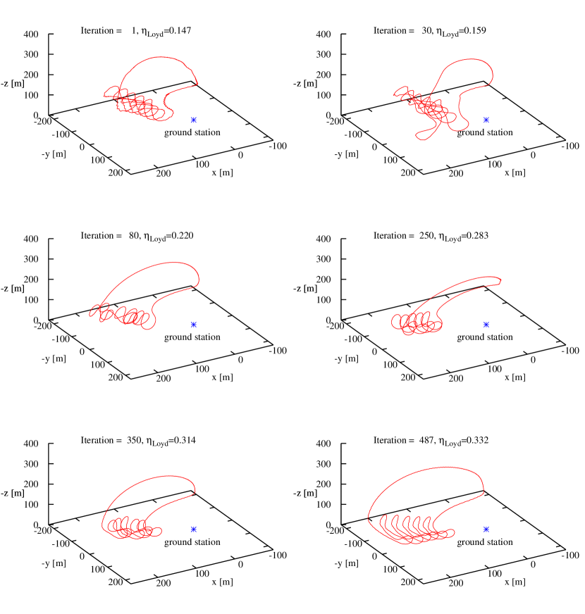
Figure 8. Evolution of pumping cycles during the optimization process. Starting with the experimentally flown trajectory (top left), the 3d trajectories for different iteration steps (number given in figure) to the optimal solution (bottom right) are shown.

It can observed that optimization starts far from optimum and runs through some crude path configurations towards the optimal solution. This behavior could be attributed to the interior point method of the used IPOPT solver.

The optimization figures of merit are given by the Loyd factor $\eta_{\rm Loyd}$, which is defined by

$$\eta_{\rm Loyd}=\frac{\bar{P}}{P_{\rm Loyd}}$$ (97)

This factor corresponds to the Loyd limit, which corresponds to the generated power $P_{\rm Loyd}$ for a kite flying ’maximal crosswind’ (at $\vartheta\!=\!0$) continuously, i.e. no retraction phase, compare (2) and [19]. For the derived model, this quantity is given by

$$P_{\rm Loyd}=\frac{\varrho C_{\rm R}A}{2}\frac{4E^{2}}{27}\frac{E}{\sqrt{1\!+\!E^{2}}}v_{\rm w}^{3}$$ (98)

The according time series for the controls and power, given as $F_{\rm tether}\dot{l}$, are presented in Fig. 9.

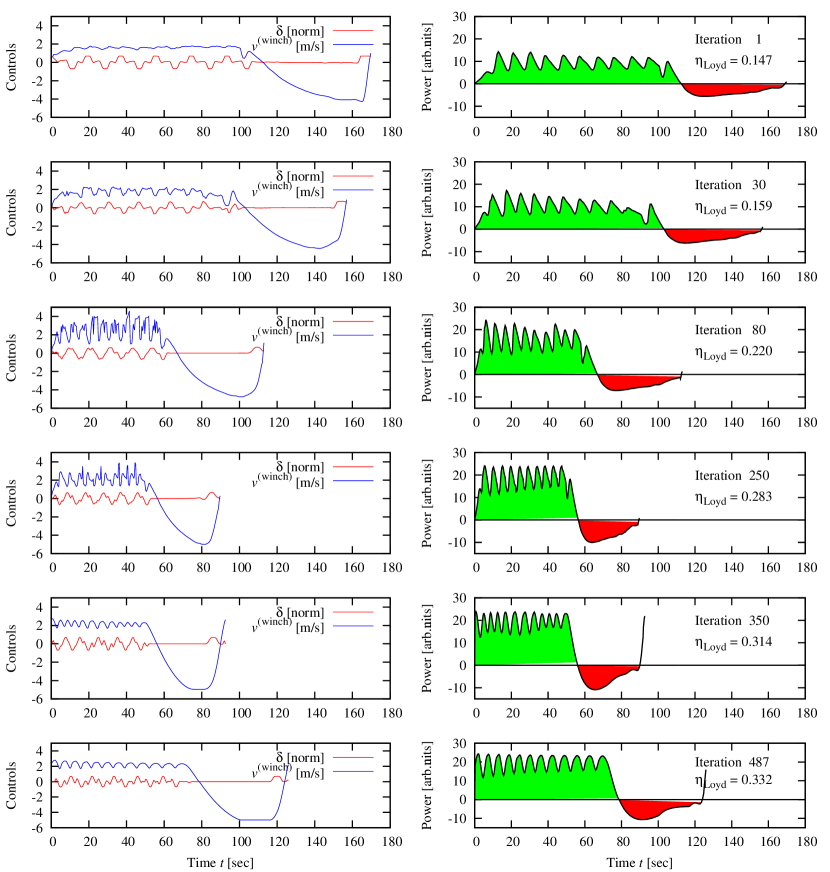
Figure 9. Time series for controls $\delta$ and $v^{\rm(winch)}$ and power, computed as tether force times reeling speed $F_{\rm tether}\dot{l}$. The upper row shows the experimentally flown pumping cycle, which is used initial guess. The lower row gives the optimal solution. Iteration numbers for the intermediate steps are annotated in the respective subplots.

In summary, it can be stated that the optimizer increased the power generation of the pumping cycle by more than a factor of two from $\eta_{\rm Loyd}\!\approx\!0.15$ to $\eta_{\rm Loyd}\!\approx\!0.33$. This is partly due to the fact that the optimized figure lies deeper in the crosswind region. Further, transfer and return phases are carried out more efficiently. The lemniscates are deformed to minimal curves fulfilling the imposed constraints. For sake of a fair assessment, it should be noted that the experimental trajectory was taken from a test flight aiming at flight controller development rather than optimal power output. Nevertheless, valuable suggestions for improvement of even these ’classical’ control setups can be extracted from such optimization results, see e.g. the winch controller implementation for the transfer phase in [12].

8. Conclusion

In conclusion, a singularity free model for tethered kite dynamics based on quaternions has been derived, which can be broadly applied for simulation and optimization purposes. It has been demonstrated that optimization runs of complete pumping cycles within a few minutes are feasible with this model. This opens up the way to further extended and systematic studies of AWE efficiencies. It should be finally remarked that these might most likely involve further extensions to the model to take into account e.g. mass effects, tether drag and a wind profile. We gratefully thank Mario Zanon for valuable discussions on the implementation of the OCP. This research was supported by KUL PFV/10/002 OPTEC; Eurostars SMART; IUAP P7 (DYSCO); EU: FP7-TEMPO (MCITN-607957), H2020-ITN AWESCO (642682) and by the ERC Starting Grant HIGHWIND (259166).

References

- [1]
- [2] U. Ahrens, M. Diehl, and R. Schmehl (eds.), Airborne Wind Energy, Green Energy and Technology (Springer Berlin Heidelberg, 2013).
- [3] J. Andersson, A General-Purpose Software Framework for Dynamic Optimization, PhD thesis, Arenberg Doctoral School, KU Leuven, Department of Electrical Engineering (ESAT/SCD) and Optimization in Engineering Center, Kasteelpark Arenberg 10, 3001-Heverlee, Belgium, October 2013.
- [4] J. Andersson, J. Ã…kesson, and M. Diehl, Casadi: A symbolic package for automatic differentiation and optimal control, in: Recent Advances in Algorithmic Differentiation, edited by S. Forth, P. Hovland, E. Phipps, J. Utke, and A. Walther, Lecture Notes in Computational Science and Engineering Vol. 87 (Springer Berlin Heidelberg, 2012), pp. 297–307.
- [5] C. Archer and K. Caldeira, Global assessment of high-altitude wind power, Energies 2, 307–319 (2009).
- [6] H. Bock and K. Plitt, A multiple shooting algorithm for direct solution of optimal control problems, in: Proceedings 9th IFAC World Congress Budapest, (Pergamon Press, 1984), pp. 242–247.
- [7] S. Costello, G. François, and D. Bonvin, Real-Time Optimization for Kites, in: Proceedings of the 5th IFAC-PSYCO Workshop, (2013), pp. 64–69.
- [8] M. Diehl, Airborne Wind Energy: Basic Concepts and Physical Foundations, in: Airborne Wind Energy, edited by U. Ahrens, M. Diehl, and R. Schmehl (Springer, 2013).
- [9] M. Erhard and H. Strauch, Control of towing kites for seagoing vessels, Control Systems Technology, IEEE Transactions on 21(5), 1629–1640 (2013).
- [10] M. Erhard and H. Strauch, Sensors and navigation algorithms for flight control of tethered kites, in: Control Conference (ECC), 2013 European, (July 2013), pp. 998–1003.
- [11] M. Erhard and H. Strauch, Theory and experimental validation of a simple comprehensible model of tethered kite dynamics used for controller design, in: Airborne Wind Energy, edited by U. Ahrens, M. Diehl, and R. SchmehlGreen Energy and Technology (Springer Berlin Heidelberg, 2013), pp. 141–165.
- [12] M. Erhard and H. Strauch, Flight control of tethered kites in autonomous pumping cycles for airborne wind energy, Control Engineering Practice 40(0), 13 – 26 (2015).
- [13] L. Fagiano and M. Milanese, Airborne wind energy: An overview, in: American Control Conference (ACC), 2012, (June 2012), pp. 3132–3143.
- [14] L. Fagiano, A. Zgraggen, M. Morari, and M. Khammash, Automatic crosswind flight of tethered wings for airborne wind energy: Modeling, control design, and experimental results, Control Systems Technology, IEEE Transactions on PP(99), 1–1 (2013).
- [15] S. Gros and M. Diehl, Modeling of airborne wind energy systems in natural coordinates, in: Airborne Wind Energy, edited by U. Ahrens, M. Diehl, and R. SchmehlGreen Energy and Technology (Springer Berlin Heidelberg, 2013), pp. 181–203.
- [16] B. Houska and M. Diehl, Optimal Control for Power Generating Kites, in: Proc. 9th European Control Conference, (Kos, Greece,, 2007), pp. 3560–3567, (CD-ROM).
- [17] C. Jehle, Automatic flight control of tethered kites for power generation, Master thesis, Technical University of Munich, Germany, 2012.
- [18] J. B. Kuipers, Quaternions and rotation Sequences: a Primer with Applications to Orbits, Aerospace, and Virtual Reality (Princeton University Press, 1999).
- [19] M. L. Loyd, Crosswind kite power, Journal of energy 4(3), 106–111 (1980).
- [20] A. Wächter and L. Biegler, On the Implementation of a Primal-Dual Interior Point Filter Line Search Algorithm for Large-Scale Nonlinear Programming, Mathematical Programming 106(1), 25–57 (2006).