Bound states of a two-dimensional electron gas in inhomogeneous magnetic fields

Abstract

We study the bound states of a two dimensional free electron gas (2DEG) subjected to a perpendicular inhomogeneous magnetic field. An analytical transfer matrix (ATM) based exact quantization formula is derived for magnetic fields that vary (arbitrarily) along one spatial direction. As illustrative examples, we consider (1) a class of symmetric power law magnetic fields confined within a strip, followed by the problem of a (2) 2DEG placed under a thin ferromagnetic film, which are hitherto unexplored. The exact Landau levels for either cases are obtained. Also, the role of the fringing magnetic field (present in the second example) on these levels is discussed.

I Introduction

The quantum mechanics of electrons constrained in two dimensions has gained a lot of interest since the advent of the (Integer) Quantum Hall and Fractional Quantum Hall Effects in the 1980s. Over the years, the experimental techniques of probing these systems with precisely structured magnetic fields at low temperatures ($\approx 100$ mK) have been perfected. Presently, magnetic fields that vary appreciably (even) in the nanometer scale can be created by fabricating thin films of (a) metal-excitable with a calculated current distribution, (b) ferromagnetic materials, (c) type-I superconducting materials, on a two-dimensional electron gas (2DEG) system. Interestingly, the magnetic field in these cases can be described in closed analytic form1 ; 2 which, is an invitation for making very precise predictions for the behavior of 2DEGs subjected to such inhomogeneous fields. However, on the theoretical side we face a setback in considering arbitrary magnetic fields, as the Schrödinger equation describing the electron-field interaction can seldom be solved analytically, except in very simple cases. Often, powerful numerical methods offer a solution to this problem, albeit, at the loss of significant physical insight.

Considering the difficulty of a generic 2DEG-magnetic field interaction problem, we focus on a select class of magnetic fields (perpendicular to the plane of the electron gas) that are confined within an infinitely long strip of width $d$. Further, if the magnetic field varies across the strip (only), remaining translation invariant along the length of the strip, an exact enumeration of the bound state energies and tunneling probabilities of the electron is possible for any form of inhomogeneity. We focus on the bound state problem here, reserving a discussion of scattering for a later paper.

Besides, a significant chunk of the literature on magnetic strips is devoted to a study of electron tunneling through the magnetic field barrier2 ; 3 ; 4 ; 5 while, relatively little is explored on the bound state solutions. Bound state solutions of a linearly varying magnetic field were obtained by Müller.3 Even in this simple case, it is not possible to describe the electron wave functions in terms of any special function or finite analytic combinations thereof. Even otherwise, bound state solutions are exceedingly special, as their existence is not necessarily guaranteed for a given magnetic field while, scattering states always exist (for any given field variation) when the energy is above a minimum threshold value. Another nontrivial field variation that enjoys exact solvability is $\mathbf{B}=1-\tanh^{2}x~{}\mathbf{e}_{z}$5 in which, the discrete and continuous part of the spectrum overlap in an energy range and are selected by the $y$ momentum associated with the wave function.

The main goal of this paper is to find the exact bound state energies (Landau levels) for any given magnetic field variation (whenever such levels exist). We formulate the problem in Section II obtaining an effective one-dimensional magnetic potential for the electron. The criterion for the allowed bound state energies is obtained with an analytic transfer matrix (ATM) approach in Section II.1. Section III is devoted to examples. Firstly, in Section III.1 we obtain the Landau levels (LLs) of a magnetic strip that has a symmetric power law field variation. Following which, we consider the problem of a 2DEG placed under a ferromagnetic film in Section III.2. Unlike in the former example, the magnetic field in this case offers a fringing field outside the strip which, has a significant effect on the LLs. We conclude in Section IV outlining avenues of further study. An appendix at the end gives the proof of an important result used in Section II.1.

II Problem formulation

We place the 2DEG on the $x$–$y$ plane, subjected to a perpendicular magnetic field

$$\mathbf{B}=B_{o}B(2x/d)\mathbf{e}_{z},\quad\zeta\mapsto B(\zeta)\neq(=)0,\quad|\zeta|\leq(>)1$$ (1)

where, $B_{o}$ is the field strength and $d$ is the width of the strip. $B(\zeta)$ must be integrable. The vector potential for this field, in the Landau gauge reads

$$\mathbf{A}=\frac{B_{o}d}{2}\Phi(2x/d)\mathbf{e}_{y},\quad\Phi(\zeta)\mathrel{\hbox to0.0pt{\raisebox{1.29167pt}{$\cdot$}\hss}\raisebox{-1.29167pt}{$\cdot$}}=\int_{-\infty}^{\zeta}{B(\zeta^{\prime}){\rm d}\zeta^{\prime}}.$$ (2)

We set up a minimal coupling Hamiltonian ${H}=({p}+e\mathbf{A})^{2}/2m^{\ast}$ to describe the electron-field interaction where, $m^{\ast}$ is the effective mass of the electron with charge $-e$. The magnetic length $\ell_{B}=\sqrt{\hslash/eB_{o}}$ and cyclotron frequency $\omega_{c}=eB_{o}/m^{\ast}$ provide natural length and time scales in this problem. Scaling the energy $E\mapsto(\hslash\omega_{c}/2)\varepsilon$ and the coordinates $(x,y)\mapsto\ell_{B}(\xi,\eta)$ we obtain the Schrödinger equation

$$\left\{{\nabla}_{\xi\eta}^{2}+i\frac{d}{\ell_{B}}\Phi\left(\frac{2\ell_{B}}{d}\xi\right)\partial_{\eta}-\left(\frac{d}{2\ell_{B}}\Phi\left(\frac{2\ell_{B}}{d}\xi\right)\right)^{2}\right\}\psi\left(\xi,\eta\right)=-\varepsilon\psi\left(\xi,\eta\right)$$ (3)

satisfied by the wave function $\psi(\xi,\eta)$. The width of the strip in $\ell_{B}$ units is given by $2\beta~{}(\beta\mathrel{\hbox to0.0pt{\raisebox{1.29167pt}{$\cdot$}\hss}\raisebox{-1.29167pt}{$\cdot$}}=d/2\ell_{B})$. Since, the Hamiltonian has a translation symmetry in the $y$ direction, the commutation identity $[{H},{p}_{y}]=0$ holds good. Thus, $\psi$ is a simultaneous eigenstate of ${H}$ and ${p}_{y}$. An ansatz $\psi(\xi,\eta)=e^{iq\eta}\varphi(\xi)$ would satisfy this requirement provided, $\varphi$ solves the one-dimensional Schrödinger equation

$$\frac{{\rm d}^{2}\varphi}{{\rm d}\xi^{2}}+\left(\varepsilon-V_{q}(\xi)\right)\varphi=0,\quad{V_{q}(\xi)\mathrel{\hbox to0.0pt{\raisebox{1.29167pt}{$\cdot$}\hss}\raisebox{-1.29167pt}{$\cdot$}}=\left(q+\beta\Phi(\xi/\beta)\right)}^{2}.$$ (4)

We call $V_{q}(\xi)$ the effective magnetic potential whose, shape is modulated by the $y$ momentum $(\hslash/\ell_{B})q$ associated with the wave function. This makes the quantum mechanical behavior wave-vector dependent.2 We will explore many interesting possibilities that arise (concerning the existence of bound states) due to the presence of $q$. Note that outside the magnetic strip i.e. $|\xi|>\beta,~{}V_{q}(\xi)$ is constant as shown in Fig. 1. Specifically, for $\xi<-\beta,~{}V_{q}(\xi)=q^{2}$, while for $\xi>\beta,V_{q}(\xi)=(q+\beta\Phi(1))^{2}$ where, $\Phi(1)$ is proportional to the magnetic flux per unit length linked with the infinite strip (see Equation (2)). Although, bound state solutions of equation  (4) can be anticipated for energies $\varepsilon<\min\left\{q^{2},(q+\beta\Phi(1))^{2}\right\}$; for a given $B(\zeta)$, the effective potential may not offer ‘wells’ for containing the electron, in which case bound state solutions will not exist for any $\varepsilon$. This shape dependence makes bound states rather scarce unlike scattering solutions.

II.1 Formally exact criterion for landau levels

In this section we use the analytic transfer matrix method (ATMM) to obtain an exact criterion for the allowed bound states in the effective potential $V_{q}(\xi)$. The ATMM emerged in the problem of finding guided modes of the electromagnetic field in a graded-index optical fiber.6 ; 7 The method was readily extended by the pioneers to apply to one-dimensional problems in quantum mechanics8 ; 9 ; 10 ; 11 ; 12 where, it has been remarkably successful not only as a calculation device for exact energy levels but also as a conceptual tool; providing deeper insights into the working and limitations of semi classical quantization schemes like the Bohr–Sommerfeld and the WKB method (and refinements of the same).10 These efforts also led to the conceptualization of the ‘modified momentum’ which, substituted for the canonical momentum makes the Bohr-Sommerfeld quantization exact.9 The ATMM, combined with super-symmetric techniques has also been applied to nontrivial potentials yielding promising results.13

In order to keep the paper self-contained, we give a complete derivation of the ATM quantization condition clarifying, a major ingredient in the derivation (the phase losses at the classical turning points) which, in our opinion has not been rigorously justified in previous accounts (Ref. appendix). Additionally, we evaluate the ATM quantization integral in closed form which, is a new development.

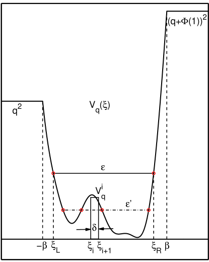
Figure 1: Sketch of the effective magnetic potential $V_{q}(\xi)$ with classical turning points $\xi_{L,R}({\color[rgb]{1,0,0}\boldsymbol{\circ}})$ for energy $\varepsilon$.

Consider two classical turning points $\xi_{L}$ and $\xi_{R}$ that solve $V_{q}(\xi)=\varepsilon$ in the region $(-\beta,\beta)$. The case of more than two turning points (as with the energy $\varepsilon^{\prime}$ in Fig. 1) is not addressed in this paper, as the ATMM is not easily generalized for multiple turning points. We partition the sub intervals $(-\beta,\xi_{L}),(\xi_{L},\xi_{R})$ and $(\xi_{R},\beta)$ into $l,m$ and $n$ segments respectively, each with width $\delta$. Thus, any intermediate point $\xi_{i}=i\delta-\beta,~{}i=0,1,2\ldots(l+m+n)$ with $\xi_{l+m+n}=\beta$. Certainly, $\xi_{L}=l\delta-\beta$ and $\xi_{R}=(l+m)\delta-\beta$. The continuous potential is now replaced by a piecewise constant equivalent over these segments, such that the potential in the segment $(\xi_{i},\xi_{i+1})$ is $V_{q}^{i}\mathrel{\hbox to0.0pt{\raisebox{1.29167pt}{$\cdot$}\hss}\raisebox{-1.29167pt}{$\cdot$}}=V_{q}\left(\frac{\xi_{i}+\xi_{i+1}}{2}\right)$. Further, the solution of equation (4) in this segment is given by

$$\varphi(\xi)=A_{i}e^{i\kappa_{i}(\xi-\xi_{i+1})}+B_{i}e^{-i\kappa_{i}(\xi-\xi_{i+1})},\quad\kappa_{i}=\sqrt{\varepsilon-V_{q}^{i}}$$ (5)

where, $A_{i}(B_{i})$ is the probability amplitude for the forward (backward) traveling wave component. In equation (5) $\varphi$ may be tagged explicitly to show the correspondence with the $i$^th segment. We prefer to infer this from the context. Necessitating the continuity of the wave function and its derivative at the endpoints of the segment we arrive at the matrix equation

$$\begin{bmatrix}\varphi(\xi_{i})\\ \dot{\varphi}(\xi_{i})\\ \end{bmatrix}=M_{i}\begin{bmatrix}\varphi(\xi_{i+1})\\ \dot{\varphi}(\xi_{i+1})\\ \end{bmatrix},~{}M_{i}=\begin{bmatrix}\cos(\kappa_{i}\delta)&-\frac{\sin(\kappa_{i}\delta)}{\kappa_{i}}\\ \kappa_{i}\sin(\kappa_{i}\delta)&\cos(\kappa_{i}\delta)\\ \end{bmatrix}$$ (6)

where, the overhead dot denotes differentiation w.r.t $\xi$. Note that $\kappa_{i}\neq 0$, since we assume no more than two classical turning points at this stage. Few authors prefer separate formulae for the transfer matrix $M_{i}$ that hold when $\varepsilon>V_{q}^{i}$ or otherwise. In view of this distinction, our expression corresponds to the former case, while the latter case i.e. $\varepsilon<V_{q}^{i}$, leading to an imaginary $\kappa_{i}$ is easily addressed with the analytic continuation of the trigonometric functions into the complex plane in equation (6). Thus, recovering the other expression for the transfer matrix when the case arises. With this caveat we overcome the need for selective indexing of transfer matrix products.

Left multiplying equation (6) with $\begin{bmatrix}-\dot{\varphi}(\xi_{i})&\varphi(\xi_{i})\end{bmatrix}$ and dividing by $\varphi(\xi_{i})\varphi(\xi_{i+1})$, we obtain

$$\begin{bmatrix}P_{i}&1\end{bmatrix}M_{i}\begin{bmatrix}1\\ -P_{i+1}\\ \end{bmatrix}=0,\qquad P_{i}\mathrel{\hbox to0.0pt{\raisebox{1.29167pt}{$\cdot$}\hss}\raisebox{-1.29167pt}{$\cdot$}}=-\frac{\dot{\varphi}(\xi_{i})}{\varphi(\xi_{i})}$$ (7)

$$\Rightarrow\frac{P_{i}}{\kappa_{i}}=\frac{\frac{P_{i+1}}{\kappa_{i}}-\tan(\kappa_{i}\delta)}{1+\frac{P_{i+1}}{\kappa_{i}}\tan(\kappa_{i}\delta)}.$$

Through the tangent addition formula we obtain

$$\frac{P_{i}}{\kappa_{i}}=\tan\left[\tan^{-1}\left(\frac{P_{i+1}}{\kappa_{i}}\right)-\kappa_{i}\delta\right]$$

$$\Rightarrow\tan^{-1}\left(\frac{P_{i}}{\kappa_{i}}\right)-\tan^{-1}\left(\frac{P_{i+1}}{\kappa_{i}}\right)=z_{i}\pi-\kappa_{i}\delta,\,$$

$$z_{i}=0,1,2,\ldots$$ (8)

Note that $P(\xi)$ satisfies the Riccati equation

$$\dot{P}=P^{2}+\varepsilon-V_{q}(\xi)=P^{2}+\kappa^{2}$$ (9)

which, has intimate connections with the Schrödinger equation 14 . It is often advantageous (as in the present case) to develop identities involving $P$. Rearranging equation (II.1) and summing over $i$ from $l+1$ to $l+m$ yields

$$\sum\limits_{i=l+1}^{l+m}{\kappa_{i}\delta}+\sum\limits_{i=l+1}^{l+m}\left[\tan^{-1}\left(\frac{P_{i+1}}{\kappa_{i+1}}\right)-\tan^{-1}\left(\frac{P_{i+1}}{\kappa_{i}}\right)\right]$$ (10)

$$\quad=N\pi+\sum\limits_{i=l+1}^{l+m}\left[\tan^{-1}\left(\frac{P_{i+1}}{\kappa_{i+1}}\right)-\tan^{-1}\left(\frac{P_{i}}{\kappa_{i}}\right)\right]$$

$$\Rightarrow\sum\limits_{i=l+1}^{l+m}{\kappa_{i}\delta}+\sum\limits_{i=l+1}^{l+m-1}\left[\tan^{-1}\left(\frac{P_{i+1}}{\kappa_{i+1}}\right)-\tan^{-1}\left(\frac{P_{i+1}}{\kappa_{i}}\right)\right]$$

$$\quad=N\pi+\tan^{-1}\left(\frac{P_{l+m+1}}{\kappa_{l+m}}\right)-\tan^{-1}{\left(\frac{P_{l+1}}{\kappa_{l+1}}\right)}$$

The exact quantization condition emerges as a limit of equation (10) as $\delta\to 0$. In the event of $\delta\to 0$, the continuous potential variation is recovered, with $P_{l+m+1}\to P(\xi_{R})$ and $P_{l+1}\to P(\xi_{L})$. In the appendix we show that $P(\xi_{L})<0<P(\xi_{R})$ and $\left|P\left(\xi_{L,R}\right)\right|<\infty$. Further, $\kappa_{l+1}\to\sqrt{\varepsilon-V_{q}(\xi_{L})}=\kappa_{l+m}\to\sqrt{\varepsilon-V_{q}(\xi_{R})}=0$ which, gives the half phase losses at the classical turning points as

$$\lim_{\delta\to 0}\tan^{-1}\left(\frac{P_{l+m+1}}{\kappa_{l+m}}\right)=-\lim_{\delta\to 0}\tan^{-1}\left(\frac{P_{l+1}}{\kappa_{l+1}}\right)=\frac{\pi}{2}.$$ (11)

Further,

$$\Delta\phi_{i} \mathrel{\hbox to0.0pt{\raisebox{1.29167pt}{$\cdot$}\hss}\raisebox{-1.29167pt}{$\cdot$}}=\tan^{-1}\left(\frac{P_{i+1}}{\kappa_{i+1}}\right)-\tan^{-1}\left(\frac{P_{i+1}}{\kappa_{i}}\right)$$

$$~{}=\tan^{-1}\left(\frac{P_{i+1}(\kappa_{i}-\kappa_{i+1})}{P_{i+1}^{2}+\kappa_{i}\kappa_{i+1}}\right)$$

$$~{}=-\frac{P_{i+1}(\kappa_{i+1}-\kappa_{i})}{P_{i+1}^{2}+\kappa_{i}\kappa_{i+1}}+\mathcal{O}\left((\kappa_{i+1}-\kappa_{i})^{3}\right)$$ (12)

which, results from expanding the inverse tangent in a tailor series in powers of $\kappa_{i+1}-\kappa_{i}$. Building on equation (12) we obtain

$$\lim_{\delta\to 0}\sum\limits_{i=l+1}^{l+m-1}{\Delta\phi_{i}}=-\lim_{\delta\to 0}\sum\limits_{i=l+1}^{l+m-1}\frac{P_{i+1}(\kappa_{i+1}-\kappa_{i})}{P_{i+1}^{2}+\kappa_{i}\kappa_{i+1}}+\lim_{\delta\to 0}\sum\limits_{i=l+1}^{l+m-1}\mathcal{O}\left((\kappa_{i+1}-\kappa_{i})^{3}\right)=-\int_{\xi_{L}}^{\xi_{R}}{\frac{P}{P^{2}+\kappa^{2}}{d}\kappa}=-\int_{\xi_{L}}^{\xi_{R}}{\frac{P}{\dot{P}}\dot{\kappa}{d}\xi}$$ (13)

using equation (9). Thus, in the limit of $\delta\to 0$, equation (10) reads

$$\int_{\xi_{L}}^{\xi_{R}}\kappa-\frac{P}{\dot{P}}\dot{\kappa}{\rm d}\xi=(N+1)\pi,\quad N=1,2,\ldots,$$ (14)

which, is an exact criteria for the bound state wave function (specified through $P$) and the corresponding energy that appears in $P$ and $\kappa$. Interestingly, the above integral can be explicitly evaluated in terms of the function

$$Q\mathrel{\hbox to0.0pt{\raisebox{1.29167pt}{$\cdot$}\hss}\raisebox{-1.29167pt}{$\cdot$}}=\frac{P}{\kappa}$$ (15)

leading to

$$\int_{\xi_{L}}^{\xi_{R}}\frac{{\rm d}Q}{1+Q^{2}} =\tan^{-1}\left(Q(\xi_{R})\right)-\tan^{-1}\left(Q(\xi_{L})\right)$$ (16)

$$=(N+1)\pi,\quad N=1,2,\ldots,$$

III Examples

III.1 Symmetric power law fields

A magnetic field that varies as a simple power law is obtained by choosing

$$B(\zeta)=\frac{1-|\zeta|^{\lambda-1}}{2}\left({{\rm sgn}}(\zeta+1)-{{\rm sgn}}(\zeta-1)\right)$$ (17)

We let $\lambda>1$ to avoid a singularity at $\zeta=0$. In the limiting event of $\lambda\to\infty$ we approach a constant magnetic field. From equation (2) we obtain

$$\Phi(\zeta)=\begin{cases}2-\frac{2}{\lambda},&\zeta\geq 1\\ \zeta+1-\frac{1}{\lambda}\left(1+{{\rm sgn}}(\zeta)|\zeta|^{\lambda}\right),&-1\leq\zeta<1\\ 0,&\zeta<-1\end{cases}$$ (18)

Substituting $\Phi$ in equation (4), we arrive at the effective magnetic potential

$$V_{q}(\xi)=\left(q+\xi+\beta-\lambda^{-1}\left(\frac{{{\rm sgn}}(\xi)}{\beta^{\lambda-1}}|\xi|^{\lambda}+\beta\right)\right)^{2}.$$ (19)

In this case only two classical turning points exist for any combination of parameters. Since $\Phi(\zeta)$ is an increasing curve, a well appears in $V_{q}(\xi)$ for $-2\beta\left(1-\frac{1}{\lambda}\right)<q<0$ (See Fig. 2). Consequently, wave functions with $q>0$ can only scatter through the magnetic field region.

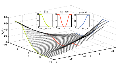
Figure 2: Surface plot of $V_{q}(\xi)$ for $\beta=5,\,\lambda=8$. In this example, wells appear when $-8.75<q<0$. (Insets) give the shapes of the highlighted regions where, the red curve (middle) corresponds to a symmetric well considered in equation (20).

Hence, we look for bound states in this range. Also (as noted before) the Landau levels (LLs) must populate the interval $0<\varepsilon<\min\left\{q^{2},\left(q+2\beta\left(1-\lambda^{-1}\right)\right)^{2}\right\}$.

For $q=-\beta\left(1-\frac{1}{\lambda}\right)$, the well becomes symmetric about the origin, described by

$$U(\xi)\mathrel{\hbox to0.0pt{\raisebox{1.29167pt}{$\cdot$}\hss}\raisebox{-1.29167pt}{$\cdot$}}=V_{\beta(1/\lambda-1)}(\xi)=\left(\xi-\frac{{{\rm sgn}}(\xi)}{\lambda\beta^{\lambda-1}}|\xi|^{\lambda}\right)^{2}~{}|\xi|<\beta.$$ (20)

We plot this symmetric-potential-well for select values of $\lambda$ in Fig. 3, with an inset displaying the variation of the well depth–given by $U(\beta)=\beta^{2}\left(1-1/\lambda\right)^{2}$–with $\lambda$. Note that the wells take a parabolic shape as $\lambda\to\infty$, which is the case with a constant magnetic field. Also, as $\beta\to\infty$, the effective well spans the entire axis becoming infinitely deep. Consequently, only bound states are permitted (as Landau had shown few decades ago).

From the bound state criterion derived above, we compute the first few LLs in this symmetric well in Fig. 4(a) and study their variation with $\lambda$. Clearly, the LLs asymptote to those of the limiting constant magnetic field which, are shown by means of broken lines in Fig. 4(a)—with increasing $\lambda$. Higher levels appear progressively, since the well-depth increases with $\lambda$ (Fig. 3 inset). We find that the highest LL$\,\sim\beta^{2}\left(1-1/\lambda\right)^{2}$. The well is always brim full! Combining this observation with the asymptotic behavior of the levels noted above gives an adequate estimate of the total number of LLs (say $N$) populating a particular well is obtained (especially as $\lambda\to\infty$).

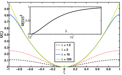
Figure 3: Plots of the effective magnetic potential $U(\xi)(=V_{(1/\lambda-1)}(\xi))$ in the region $-1<\xi<1$, $\beta=1$. (Inset) gives the asymptotic levelling of the well-depth in the event of $\lambda\to\infty$.

$$2N\sim\beta^{2}\left(1-\frac{1}{\lambda}\right)^{2}+1.$$ (21)

In Fig. 4(b) we superpose the LLS of the previous case with those corresponding to a larger $\beta=10$. Numerous higher levels (red dots) appear due to the increase in the well-depth. Further, with increasing $\lambda$, the LLs for either values of $\beta$ almost overlap which is emphasized by the boxed region in Fig. 4(b).

Note that, even in the limit of $\lambda\to\infty$ (describing a constant magnetic field) the width of the strip remains finite (since $\beta$ is fixed); quite insensitive to which, the LLs asymptote to the LLs of a spatially-unbounded uniform field (the Landau Problem). We recall that in the former case the wave functions outside the strip decay exponentially (since the effective potential is constant out side the strip) while, those in the latter case have Gaussian tails. It thus turns out, despite a finite width, the LLs overwhelmingly approach those of the spatially-unbounded uniform magnetic field for large enough values of $\lambda$.

III.2 2DEG under a ferromagnetic film

The symmetric power law magnetic fields considered above cannot be realized with the experimental methods discussed in Section I. However, they serve as good approximations to realistic magnetic fields. A crucial element that lacks in these ideal geometries is the presence of a fringing field outside the strip. For large sample sizes the fringing field can often be neglected. In this spirit, we had required that the magnetic field be strictly zero outside the strip (equation (1)). Consequently, $V_{q}(\xi)$ became constant for $|\xi|>\beta$, and an exact criterion for the LLs could be obtained.

Now, we relax this constraint and allow the field to out-flank the strip; with an understanding that the field vanishes progressively with distance from the strip. For these fields, most of the treatment remains same as before, except for a truncation of the effective potential far away from the classical turning points, which turns out to be a valid approximation, if the LL under consideration is much below the height of the effective potential at the truncation points.11 ; 12 The consequent error can be overcome by choosing truncation points sufficiently far from the turning points, allowing the LLs of interest to settle within the desired precision.

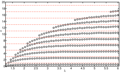
(a)

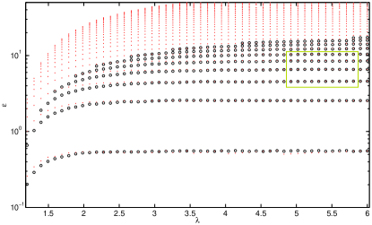
(b)

Figure 4: Plot of first few LLs (black circles) corresponding to different $\lambda$ for $\beta=5$. Horizontal broken lines give the LLs for a uniform, infinitely extending magnetic field ($LL_{l+1}=2l+1,l=0,1,2\ldots)$ (b) Black circles are same as that in (a), while red dots give the LLs for $\beta=10$.

Consider a 2DEG placed under a ferromagnetic film at a distance $z$ below it. For a vertically magnetized film of width (thickness) $d(a)$ and magnetization per unit width $\sigma$, the magnetic field on the 2DEG is given by

$$\mathbf{B}(x,z)=B_{o}B(\zeta)\mathbf{e}_{z},$$

$$B(\zeta)=2\left\{\frac{(\zeta+1)}{(\zeta+1)^{2}+z_{o}^{2}}-\frac{(\zeta-1)}{(\zeta-1)^{2}+z_{o}^{2}}\right\},$$

$$B_{o}\mathrel{\hbox to0.0pt{\raisebox{1.29167pt}{$\cdot$}\hss}\raisebox{-1.29167pt}{$\cdot$}}=2a\sigma,~{}z_{o}=2\frac{z}{d}$$ (22)

when, $a/d,a/z\ll 1$.2 The length of the strip is infinite as before. Using equation (2) we obtain

$$\Phi(\zeta)=\ln\left(\frac{(\zeta+1)^{2}+z_{o}^{2}}{(\zeta-1)^{2}+z_{o}^{2}}\right)$$ (23)

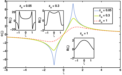
Figure 5: Plot of $\Phi(\zeta)$ vs. $\zeta$ for $z_{o}=0.05,~{}0.3,~{}1$. (Insets) show the magnetic field variation $B(\zeta)$ for these values of $z_{o}$.

which, leads to the effective magnetic potential

$$V_{q}(\xi)=\left\{q+\beta\ln\left(\frac{(\xi+\beta)^{2}+\theta^{2}}{(\xi-\beta)^{2}+\theta^{2}}\right)\right\}^{2}$$ (24)

In obtaining the effective potential we scaled $z=\ell_{B}\theta$ and used the definition $z_{o}=2z/d=(2l_{B}/d)\theta=\theta/\beta$.

Due to the interplay of the parameters describing the effective-potential, many interesting possibilities arise. First of all, unlike in the former example, $V_{q}(\xi)$ varies (appreciably) over the entire $\xi$ axis tending to $q^{2}$ as $|\xi|\to\infty$. Secondly, the effective potential in this case possesses a special reflection symmetry $V_{-q}(\xi)=V_{q}(-\xi)$, which implies that the energy eigenvalues of equation (4) for bound state solutions remain invariant under the transformation $q\mapsto-q$. Thus, the LLs are doubly degenerate. From this property, it suffices to study the spectrum for $q>0$. Further, for an energy $\varepsilon$, there can exist at the most four classical turning points given by

$$\xi=-\beta\coth\phi_{\pm}\pm\left(\beta^{2}{{\rm csch}}^{2}\phi_{\pm}-\theta^{2}\right)^{\frac{1}{2}}~{}~{}\phi_{\pm}=\frac{q\pm\sqrt{\varepsilon}}{2\beta}$$ (25)

one or more of which might vanish–in the event of $\phi_{+},\phi_{-}=\ln\left(\beta/\theta\pm\sqrt{1+(\beta/\theta)^{2}}\right)$–get repeated or become complex. In the interest of bound states, four (distinct) turning points may correspond to an energy within a double-well shaped potential, while two repeated (coincident) turning points would occur when the energy hits the top of the barrier between the two wells. And, higher energies would give rise to (only) two real turning points. These cases are illustrated in Fig. 6(a). A clearer perspective of the ‘motion’ of the tuning points (in the complex $\xi$ plane) is obtained by examining their loci (Ref. Fig. 6(b)) parameterized by the energy.

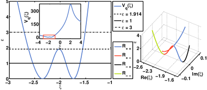
Figure 6: (a) Plot of $V_{q}(\xi)$ vs. $\xi$ for $\beta=2,~{}\theta=0.3,~{}q=9$ showing a double-well potential. Horizontal energy lines intersect the potential at the (real) classical turning points. (Inset) displays the same potential on a larger range of $\xi$. (b) Loci of the classical turning points $R_{ab}=-\beta\coth\phi_{a}+b\left(\beta^{2}{{\rm csch}}^{2}\phi_{a}-\theta^{2}\right)^{1/2},~{}ab=\pm$ (Ref. equation (24)) parameterized by $\varepsilon$ taken along an axis perpendicular to the complex $\xi$ plane.

Next, we discuss the LLs supported by the effective potential. At the present moment the correct generalization of the ATMM criterion for more than two classical turning points is not clear, which prevents us from obtaining the LLs (lying below the barrier top) for the double well shown in Fig. 6(a). However, the interested reader is referred to the work of L. V. Chebotarev on the ‘Extensions of the Bohr–Sommerfeld formula to double- well potentials’15 which, can be used to find the (approximate) LLs for this case.

In the event of $\theta>\beta,~{}q>2\beta\tanh^{-1}(\beta/\theta)$ the effective potential (in this case) offers a single well (Ref. Fig. 7(a)) with two classical turning points at $\xi=-\beta\coth\phi_{-}\pm\left(\beta^{2}{{\rm csch}}^{2}\phi_{-}-\theta^{2}\right)^{1/2}$. The LLs in this case can be computed with our ATM quantization criterion. Using equation (4) we obtain the LLs for this single well which, are plotted in Fig. 7(b) for various values of $q$. Note that as $q$ increases, the minimum value (bottom) of the effective potential $\min(V_{q})$, also increases, hence the lowest Landau levels increase in energy. In fact, the well depth, i.e. $q^{2}-\min(V_{q})$ also increases with $q$, unfolding higher LLs. However, the rate of emergence of new LLs becomes slower with increasing $q$ as shown in Fig. 7(b) inset.

Before concluding, we discuss the effect of the fringing magnetic field pervading the region outside the strip, i.e. $|\xi|>\beta$. Generally, with increasing distance from the ferromagnetic film, i.e. $\theta\gg\beta$ the fringing field can be neglected. However, the fringing field itself gave rise to many interesting effective potential shapes (unlike in the previous example). Particularly, in the preceding single well case with $\theta=2\beta$, we find that the effective well manifests in the interval $-5\beta<\xi<0$, which lies outside the strip. This also gives a clue as to where the probability density of the electron is likely to be accumulated.

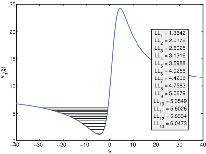
(a) Effective magnetic potential $V_{q}(\xi)$ for $\beta=2$, $\theta=4$, $q=3$ with 13 LLs depicted by horizontal lines.

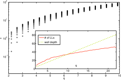
(b) Plot of allowed LLs with $\beta=2$, $\theta=4$ and $q>2\beta\tanh^{-1}(\beta/\theta)\sim 2.197$. (Inset) Plot of # of LLs and the well depth $=q^{2}-\min(V_{q})$ vs. $q$.

Figure 7:

IV Conclusion

In this paper we considered the problem of finding the bound state solutions of an infinite 2DEG subjected to a perpendicular magnetic field that varies (arbitrarily) in one direction only. An exact criterion for the bound state energies or Landau levels was developed using the analytic transfer matrix method (ATMM) for the case when the effective magnetic potential allowed two (real) classical turning points. The extensions of the ATMM for more than two turning points is not clear at the present moment and calls for further consideration. Applying our formalism to a symmetric power law magnetic field led to the exact LLs, whose variation with the strip-width $\beta$ and field exponent $\lambda$ were studied. In the sequel we looked at a 2DEG placed under a ferromagnetic film, which is an experimentally realizable system. Fortunately, this example could be tracked analytically to a great extent and the LLs for a single (effective) well were obtained for various values of the $y$-momentum $(\hbar/\ell_{B})q$. This example also emphasized the role of the fringing field on the Landau levels.

Acknowledgements: I gratefully acknowledge the help of Prof. Dr. Hemalatha Thiagarajan whose, meticulous proofreading drew my attention to many errors which, I believe have been corrected. I also benefited from the discussions with Dr. Sumiran Pujari on the ATM quantization formula.

*

Appendix A

Let $\psi(x)$ be a bound state solution of the one-dimensional Schrödinger equation

$$\frac{{\rm d}^{2}\psi}{{\rm d}x^{2}}+(E-V(x))\psi=0.$$ (1)

Based on the properties of an admissible bound state wave function we deduce an important property of the auxiliary function

$$P(x)=-\psi^{-1}\frac{{\rm d}\psi}{{\rm d}x}$$ (2)

which, is well defined (and bounded) at any finite $x$ excepting the nodes of the wave function. We show that

$$P(x)<(>)0,\qquad x=x_{L}\left(x_{R}\right)$$ (3)

at the left (right) most classical turning point $x_{L}(x_{R})$ that solves $V(x)=E$. Using this result we obtain the half phase loss at the turning point $x_{R}(x_{L})$ to be $+\left(-\right)\frac{\pi}{2}$. It is implicit that we are working with a real $\psi$, hence the inequality in proposition (3) is valid.

Proof: The points where $V(x)<(>)E$ constitute the classically allowed (forbidden) region. Consider the following properties

1. $|\psi|\to 0,|\psi^{\prime}|\to 0$ as $|x|\to\infty$

2. $\psi\neq 0$ for any $x$ (no nodes) in the classically forbidden region

which, hold good for any bound state wave function. Since, equation (1) is form invariant under the transformation $x\mapsto-x(\Rightarrow x_{L}\mapsto x_{R})$ while ${\rm d}/{\rm d}(-x)\mapsto-{\rm d}/{\rm d}(-x)$, it suffices to prove any one of the two propositions in (3). We focus on the left most classical turning point $x_{L}$. The truth of proposition (3) at this point rejects the possibility ${\rm sgn}\left[\psi(x_{L})\right]=-{{\rm sgn}}\left[\psi^{\prime}(x_{L})\right]$; ${\rm sgn}[~{}]$ being the signum function. To prove this we let $\psi(x_{L})>0>\psi^{\prime}(x_{L})$. From property 2, it follows that $\psi(x)>0$ for all $x<x_{L}$ (a classically forbidden region). Therefore, $\psi^{{}^{\prime\prime}}>0$ (from equation (1)–(2)). Since, $\psi$ is increasing (away from the origin) at $x_{L}$, it must attain at least one maxima before it asymptotes to the real axis (as $x\to-\infty)$ remaining positive-definite all along. Clearly, at the site of this maximum $\psi^{{}^{\prime\prime}}<0$ which is not possible. The other possibility $\psi(x_{L})<0<\psi^{\prime}(x_{L})$ (a ‘reflection’ of the previous case) is readily contradicted from form-invariance of equations (1)–(2) under the transformation $\psi\mapsto-\psi$.

Finally, we show that

$$|P(x_{L,R})|<\infty$$ (4)

Proof: Since, $\psi$ and $\psi^{\prime}$ cannot vanish simultaneously, note2 we need only show that a classical turning point cannot be a node of the wave function. Consider $x_{L}$ as before. Assume $\psi^{\prime}(x_{L})\neq\psi(x_{L})=0$. From property 1, $\psi\to 0$ as $x\to-\infty$. Thus, $\psi$ must admit at least one minima (maxima) if $\psi^{\prime}(x_{L})<0(>0)$ remaining negative (positive) definite all along. However, this contradicts the fact that $-\infty<x<x_{L}$ is classically forbidden.

References

- (1) A. Nogaret, Electron dynamics in inhomogeneous magnetic fields. Journal of Physics: Condensed Matter, 22(25), 253201 (2010).
- (2) A. Matulis, F. M. Peeters, & P. Vasilopoulos, Wave-vector-dependent tunneling through magnetic barriers. Physical review letters, 72(10), 1518 (1994).
- (3) J. E. Müller, Effect of a nonuniform magnetic field on a two-dimensional electron gas in the ballistic regime. Physical review letters, 68(3), 385 (1992).
- (4) Y. Guo, H. Wang, B. L. Gu, & Y. Kawazoe, Electric-field effects on electronic tunneling transport in magnetic barrier structures. Physical Review B, 61(3), 1728 (2000).
- (5) M. Calvo, Exactly soluble two-dimensional electron gas in a magnetic-field barrier. Physical Review B, 48(4), 2365 (1993).
- (6) Z. Cao, Y. Jiang, Q. Shen, X. Dou, & Y. Chen, Exact analytical method for planar optical waveguides with arbitrary index profile. JOSA A, 16(9), 2209–2212 (1999).
- (7) Z. Cao, Q. Liu, Y. Jiang, Q. Shen, X. Dou, & Y. Ozaki, Phase shift at a turning point in a planar optical waveguide. JOSA A, 18(9), 2161–2163 (2001).
- (8) Z. Cao, Q. Liu, Q. Shen, X. Dou, Y. Chen, & Y. Ozaki, Quantization scheme for arbitrary one-dimensional potential wells. Physical Review A, 63(5), 054103 (2001).
- (9) Z. Liang, Z. Q. Cao, X. X. Deng, & Q. S. Shen, Generalized quantization condition, 22(10), 2465–2468 (2005).
- (10) Z. Cao, & C. Yin, Advances in One-Dimensional Wave Mechanics. Springer (2014).
- (11) A. Hutem, & C. Sricheewin, Ground-state energy eigenvalue calculation of the quantum mechanical well via analytical transfer matrix method. European Journal of Physics, 29(3), 577 (2008).
- (12) H. Ying, Z. Fan-Ming, Y. Yan-Fang, & L. Chun-Fang, Energy eigenvalues from an analytical transfer matrix method. Chinese Physics B, 19(4), 040306 (2010).
- (13) H. Sun, The Morse potential eigenenergy by the analytical transfer matrix method. Physics Letters A, 338(3), 309–314 (2005).
- (14) S. B. Haley, An underrated entanglement: Riccati and Schrödinger equations. American Journal of Physics, 65(3), 237–243 (1997).
- (15) L. V. Chebotarev, Extensions of the Bohr–Sommerfeld formula to double-well potentials. American Journal of Physics, 66(12), 1086–1095 (1998).
- (16) For a bound state wave function , if at any finite (with , then must vanish identically.