Topologically nontrivial Hofstadter bands on the kagome lattice

Abstract

We investigate how the multiple bands of fermions on a crystal lattice evolve if a magnetic field is added which does not increase the number of bands. The kagome lattice is studied as generic example for a lattice with loops of three bonds. Finite Chern numbers occur as a nontrivial topological property in the presence of the magnetic field. The symmetries and periodicities as a function of the applied field are discussed. Strikingly, the dispersions of the edge states depend crucially on the precise shape of the boundary. This suggests that suitable design of the boundaries helps to tune physical properties which may even differ between upper and lower edges. Moreover, we suggest a promising gauge to realize this model in optical lattices.

I Introduction

Since the discovery of the quantum Hall effects v. Klitzing et al. (1980); Tsui et al. (1982), interest in topological aspects of condensed-matter systems has risen and has stayed very high ever since. The link to topological invariants is given by the Berry phase Berry (1984) of the ground-state wave function in its dependence of magnetic fluxes on a torus Niu et al. (1985); Wegner (1988). This line of argument even shows that there are no corrections to Ohm’s law on the linear relationship between voltage and current Klein and Seiler (1990); Uhrig (1991).

Only a few years ago, the discovery of topological insulators Ando (2013) gave another impetus to the field of topology in condensed-matter physics. Even in classical mechanical systems topological edges states can be excited Süsstrunk and Huber (2015). Very recently, topologically nontrivial bands were realized in lattices of ultracold atoms Jiménez-García et al. (2012); Aidelsburger et al. (2015) and advocated in strongly frustrated spin systems with Dzyaloshinskii-Moriya interactions Romhányi et al. (2015).

For the present article, we are inspired by the realization of nontrivial gauge fields in optical lattices filled by ultracold atoms Jiménez-García et al. (2012); Aidelsburger et al. (2015) and by the interest in nontrivial lattices. Whereas Aidelsburger et al. realized bands with Chern numbers different from zero in Bravais lattices, we show that similar physics also occurs in crystal lattices, i.e., lattices with a basis. Moreover, our focus is on lattices with loops of odd numbers of bonds. The generic loop is a triangle which has the smallest odd number of bonds. In antiferromagnetic spin systems, it is the prime source of frustration.

In our theoretical study, we aim at a proof-of-principle result. Though inspired by the impressive recent advances in systems of ultracold atoms in optical lattices Jiménez-García et al. (2012); Aidelsburger et al. (2015); Jotzu et al. (2014), we do not claim that this class of systems provides the most promising candidate for experimental realizations. The obstacle may be that the traps constructed so far do not provide well-defined edges, which we examine below. But solid-state systems may fill the gap. The recent observation of the quantum anomalous Hall effect in thin layers for ferromagnetic Chern insulators provides seminal progress Chang et al. (2013); Kou et al. (2014). Presently, higher temperatures are reached at which the effect occurs Chang et al. (2015) and theoretical calculations even suggest that in tailored systems experiments at room temperature are possible Wu et al. (2014); Han et al. (2015). There are concrete suggestions for tailored superlattices which should also make the design of particular edges possible Krasheninnikov and Nieminen (2011); Han et al. (2015). An alternative to solid-state lattices may be the artificial lattices built from dots or antidots in tailored semiconductor structures Lan and Ding (2012).

In the present fundamental investigation, we study the kagome lattice shown in Fig. 1. This crystal lattice has a basis of three atoms, labeled A, B, and C in the sketch. One choice of primitive vectors is shown; they span a parallelogram which constitutes a unit cell. Note that the coordination number is only $z=4$ which is rather low in comparison to $z=6$ for the triangular lattice, the generic Bravais lattice with triangular loops. This lattice has appeared before in several studies. In particular, we show that the kagome lattice in certain magnetic fields corresponds to special cases of Haldane models Haldane (1988), i.e., models without uniform magnetic field but complex hoppings, on the kagome lattice Ohgushi et al. (2000); Katsura et al. (2010); Tang et al. (2011). Moreover, in the research field investigating flat band models and interaction effects on them the kagome lattice is also studied intensively; for a review see Ref. Bergholtz and Liu (2013).

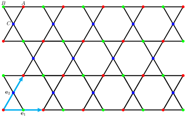
Figure 1: (Color online) Sketch of the kagome lattice, which is a crystal lattice with a basis of three sites (A, B, and C). Also shown is one choice of primitive vectors $\textbf{e}_{i}$ (in light blue) which span the unit cell.

We study this model for the special magnetic fields where the number of bands still equals the number of bands without magnetic field. Note that this is an important difference from the investigation of the square lattice by Aidelsburger et al. where topological effects could only arise once the number of bands was increased by certain values of the magnetic field Aidelsburger et al. (2015). The bands and their dispersion are computed as well as the first Chern number $C_{n}$. This Chern number equals the Berry phase Berry (1984) occurring for a Bloch state which surrounds the Brillouin zone. The Brillouin zone is the relevant two-dimensional manifold, namely, a simple torus $T^{2}$. This Chern number is defined by

$$C_{n}:=\frac{1}{2\pi\mathrm{i}}\int_{T^{2}}F^{(n)}df\quad\in\mathbb{Z}$$ (1a)

$$=\frac{1}{2\pi\mathrm{i}}\int_{T^{2}}(\langle\partial_{1}u_{n\textbf{k}}|\partial_{2}u_{n\textbf{k}}\rangle-\langle\partial_{2}u_{n\textbf{k}}|\partial_{1}u_{n\textbf{k}}\rangle)dk_{1}dk_{2}.\qquad$$ (1b)

In Eq. (1a) $F^{(n)}$ is the Berry curvature Berry (1984) of the principal $U(1)$ fiber bundle defined by the $n$th Bloch eigenstate over the Brillouin zone. Equation (1b) is the explicit formula in terms of the Bloch states $|u_{n\textbf{k}}\rangle$. The partial derivatives $\partial_{i}$ refer to the derivation with respect to the momenta $k_{i}$, i.e., $\partial_{i}:=\partial/\partial k_{i}$. The above Chern number must be an integer since it can be converted by the Stokes theorem to the integrated phase along a closed path divided by $2\pi$.

We compute the above Chern number for the three kagome bands, thereby identifying the topologically nontrivial bands.

II Model and magnetic fields

For simplicity, we study a nearest-neighbor tight-binding model on the kagome lattice. Its Hamiltonian reads

$$\hat{H}=\sum_{\langle ij\rangle}t_{ij}c^{\dagger}_{i}c_{j}+\sum_{i}V_{i}c^{\dagger}_{i}c_{i}$$ (2)

where the indices run over all sites and $\langle ij\rangle$ stands for nearest neighbors. The creation operator $c^{\dagger}_{i}$ creates a fermion at site $i$ and $c_{i}$ annihilates it. In general, we consider complex hopping elements $t_{ij}=t\exp(i\vartheta_{ij})$ with some directed phases $\vartheta_{ij}$ resulting from the Peierls substitution, i.e.,

$$\vartheta_{ij}=\frac{q}{\hbar}\int_{i}^{j}\textbf{A}\,d\textbf{r},$$ (3)

where $q$ is the charge of the hopping particle. The local potentials are given by $V_{i}$. They depend on the sublattice to which the site $i$ belongs.

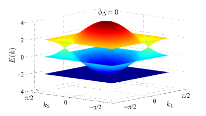
Figure 2: (Color online) Dispersion of the three bands as functions of $k_{1}$ and $k_{2}$ as defined in Eq. (5) in the kagome lattice without any magnetic field and local potentials. The hopping is set to $t=1$. Note the flat lowest band and the two Dirac cones where the two other bands touch with linear dispersion.

As a reference, we first look at the case without any magnetic fields and without local potentials such that $\vartheta_{ij}=0$ and $V_{i}=0$. It is known that in this case a flat band occurs because the kagome lattice is a line graph, namely, the line graph of the honeycomb lattice. Line graphs are generally known to have flat bands Mielke (1991a, b). The explicit calculation illustrates the flat band nicely in Fig. 2. It is based on the $3\times 3$ matrix in momentum space

$$\mathcal{H}_{\textbf{k}}=2t\begin{pmatrix}0&\cos k_{1}&\cos k_{2}\\ \cos k_{1}&0&\cos k_{3}\\ \cos k_{2}&\cos k_{3}&0\\ \end{pmatrix},$$ (4)

where we use the wave-vector components

$$k_{i} := \textbf{k}\cdot\mathbf{\Delta}_{i},$$ (5a)

$$\mathbf{\Delta}_{1} := \textbf{e}_{1}/2,$$ (5b)

$$\mathbf{\Delta}_{2} := \textbf{e}_{2}/2,$$ (5c)

$$\mathbf{\Delta}_{3} := \mathbf{\Delta}_{2}-\mathbf{\Delta}_{1}$$ (5d)

with $\textbf{e}_{1}=(1,0)^{\dagger}$ and $\textbf{e}_{2}=(1,\sqrt{3})^{\dagger}/2$; i.e., the lattice constant from one A site to the nearest A site is set to unity. We stress that the full Brillouin zone is given by $k_{i}\in[-\pi/2,\pi/2]$ because the $\mathbf{\Delta}_{i}$ have only half the length of the primitive vectors. Note that $k_{3}=k_{2}-k_{1}$ holds according to the above definitions; only two of the $k_{i}$ are independent.

The energy eigenvalues of the matrix (4) are

$$E_{1,2\textbf{k}} = t(1\pm\sqrt{1+8\cos k_{1}\cos k_{2}\cos k_{3}}\,),$$ (6a)

$$E_{3\textbf{k}} = -2t.$$ (6b)

These bands are degenerate at $\textbf{k}=(0,0)^{\dagger}$ where the flat band touches the lower dispersive band and at $\textbf{k}_{\pm}=\pm(2\pi/3)(1,-\sqrt{3})^{\dagger}$ where the two dispersive bands display Dirac cones. Due to the degeneracy, the Chern numbers $C_{n}$ of the bands are not properly defined. But even if one breaks the degeneracy, for instance by infinitesimal local potentials, the $C_{n}$ turn out to be trivial, i.e., zero, because the model without finite phases is time-reversal invariant which implies $C_{n}=0$.

Thus we turn to the model in a uniform magnetic field perpendicular to the kagome plane. This induces finite phases according to Eq. (3). We do not aim at discussing the complete intricate interplay of discrete lattice symmetry and noncommuting magnetic translations Zak (1964a, b); Kohmoto (1985) which give rise to multiple Hofstadter bands Hofstadter (1976). Instead, we aim at the situation where the magnetic translations $T_{i}$ along the primitive vectors $\textbf{e}_{i}$ commute. They obey the relation $T_{1}T_{2}=\exp(i\phi_{\text{UC}})T_{2}T_{1}$ where $\phi_{\text{UC}}$ is the magnetic flux through the unit cell measured in units of $\hbar/e$ Zak (1964a, b); Kohmoto (1985). Thus, in order not to increase the number of bands, we avoid decreasing the translational symmetry. Thus we focus on the commuting case $T_{1}T_{2}=T_{2}T_{1}$ implying

$$\phi_{\text{UC}}=2\pi n,$$ (7)

where $n\in\mathbb{Z}$ is an arbitrary integer. Inspecting the unit cell shown by the lightly shaded area in Fig. 3 elementary geometry shows that $\phi_{\text{UC}}=8\phi_{\Delta}$ if $\phi_{\Delta}$ is the flux through a triangle. Thus Eq. (7) translates to

$$\phi_{\Delta}=\frac{\pi}{4}n.$$ (8)

The physics modulo gauge transformations of the phases is only influenced by the fluxes through the loops modulo flux quanta, not by the individual phases. Thus we conclude that the physics, such as Chern numbers of the bands, depends on $\phi_{\Delta}$ with periodicity of $2\pi$ so that we will have to study only the values of $n$ modulo 8.

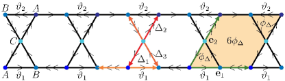
Figure 3: (Color online) Gauge chosen for the specific calculations. Two phases, $\vartheta_{1}$ and $\vartheta_{2}$, are introduced which are directed in the sense of the arrows.

We choose a specific gauge where the phases $\vartheta_{ij}$ take values as depicted in Fig. 3. The arrows on the bonds stand for the direction of the phases $\vartheta_{1}$ and $\vartheta_{2}$. In this gauge, the total phase around the unit cell takes the value zero, which may be a surprise because it seems to reflect zero flux and thus zero magnetic field. But this is not the case because the sum of all phases along closed loops is meaningful only modulo $2\pi$. Hence zero total phase complies with a finite flux fulfilling Eq. (7). To make this point explicit we consider a gauge for arbitrary flux in Appendix A and show that it can be regauged to the one in Fig. 3 in Appendix B. In this particular gauge, the relation between these phases and the flux $\phi_{\Delta}$ is the following

$$3\vartheta_{1} = \phi_{\Delta}-2\pi\,m_{1},$$ (9a)

$$3\vartheta_{2} = \phi_{\Delta}-2\pi\,m_{2},$$ (9b)

$$-3(\vartheta_{1}+\vartheta_{2}) = 6\phi_{\Delta}-2\pi\,m_{3},$$ (9c)

$$0 = 8\phi_{\Delta}-2\pi\,n,$$ (9d)

where $m_{i}$ and $n\in\mathbb{Z}$ may occur since the fluxes through the loops are only fixed up to multiples of $2\pi$. The last equation [Eq.(9d)] is the sum of the three equations before with $n=m_{1}+m_{2}+m_{3}$ which confirms Eq. (7). The left-hand side of Eq. (9d) stands for the vanishing sum of all phases around a unit cell; see Fig. 3. This does not mean that there is no net uniform magnetic field through the lattice, but it reflects the fact that the magnetic translations commute for the special magnetic fields we are considering because the flux through the unit cell is a multiple of the flux quantum. Thus, there are gauges without net total phase around the unit cells and we are employing such a gauge here for simplicity. But in the smaller loops, i.e., the triangles, there is a net flux given by $\phi_{\Delta}$.

For finite phases and local potentials we obtain the following matrix problem:

$$\mathcal{H}_{\textbf{k}}=\begin{pmatrix}V_{A}&2te^{-\mathrm{i}\bar{\vartheta}}c_{1}&2te^{\mathrm{i}\bar{\vartheta}}c_{2}\\ 2te^{\mathrm{i}\bar{\vartheta}}c_{1}&V_{B}&2te^{-\mathrm{i}\bar{\vartheta}}c_{3}\\ 2te^{-\mathrm{i}\bar{\vartheta}}c_{2}&2te^{\mathrm{i}\bar{\vartheta}}c_{3}&V_{C}\\ \end{pmatrix},$$ (10)

where we use the shorthand

$$c_{i}:=\cos(k_{i}-(-1)^{i}\Delta\vartheta)$$ (11)

for brevity. We have introduced the average and the difference of the phases $\bar{\vartheta}:=(\vartheta_{1}+\vartheta_{2})/2$ and $\Delta\vartheta:=(\vartheta_{1}-\vartheta_{2})/2$. Obviously, the matrix $\mathcal{H}_{\textbf{k}}$ is $2\pi$ periodic in $\bar{\vartheta}$ and $\Delta\vartheta$. Interestingly, the band Hamiltonian (10) is identical to the ones considered in Haldane models before Ohgushi et al. (2000); Katsura et al. (2010); Tang et al. (2011) if $\Delta\vartheta=0$ and the local potentials are switched off. But we recall that Eq. (10) only holds for uniform magnetic fields which meet the condition (8). This observation leads us to the experimentally useful result that certain Haldane models can be realized for specific fluxes complying with Eq. (8) by uniform magnetic fields.

But the eigenvalues are even periodic in $\bar{\vartheta}$ with period $2\pi/3$. This can be seen by the gauge transformation

$$\mathcal{U}=\begin{pmatrix}1&0&0\\ 0&e^{\mathrm{i}2\pi/3}&0\\ 0&0&e^{\mathrm{i}4\pi/3}\\ \end{pmatrix},$$ (12)

which transforms the Hamiltonian matrix according to

$$\mathcal{H}_{\textbf{k}}(\bar{\vartheta}+2\pi/3)=\mathcal{U}\mathcal{H}_{\textbf{k}}(\bar{\vartheta})\mathcal{U}^{\dagger}.$$ (13)

The value of $\Delta\vartheta$ remains unchanged. Clearly, the eigenvalues at each momentum do not change under the transformation and hence they are $2\pi/3$-periodic in $\bar{\vartheta}$. Since the transformation $\mathcal{U}$ is independent of momentum it does not change the Chern numbers either so that the Chern numbers are also $2\pi/3$-periodic. Note that a change of $\bar{\vartheta}$ by $2\pi/3$ at constant $\Delta\vartheta$ corresponds to the simultaneous change

$$m_{1}\to m_{1}-1,m_{2}\to m_{2}-1,\quad\text{and}\quad m_{3}\to m_{3}+2.$$ (14)

Alternatively, the increase of $\bar{\vartheta}$ by $2\pi/3$ can be interpreted as an increase of $\phi_{\Delta}$ by $2\pi$ and the increment $m_{3}\to m_{2}+8$. Thus, we see that the physics is indeed $2\pi$-periodic in $\phi_{\Delta}$.

In addition, one easily sees that $\bar{\vartheta}\to\bar{\vartheta}+\pi$ simply leads to a global minus sign in the Hamiltonian matrix (10), thus inverting the sequence of bands and thereby swapping the Chern numbers of the first and the third bands. The change $\bar{\vartheta}\to\bar{\vartheta}+\pi$ directly corresponds to the change $\phi_{\Delta}\to\phi_{\Delta}+3\pi$; see Eq. (9). But in view of the $2\pi$-periodicity in $\phi_{\Delta}$ we find the corresponding bands up to a gauge transformation already for $\phi_{\Delta}\to\phi_{\Delta}+\pi$. For examples, we refer the reader to the Sec. III below.

Moreover, reversing time amounts up to changing the sign of the phases $\vartheta_{i}\to-\vartheta_{i}$ and of the flux $\phi_{\Delta}\to-\phi_{\Delta}$; i.e., the Hamiltonian matrix is complex conjugated. This transformation of $\mathcal{H}_{\textbf{k}}$ leaves the eigenvalues and, thus the dispersion unchanged because the energy eigenvalues are real numbers. But it changes the sign of the Chern numbers.

Combined with the shift of the flux by $\pi$ we obtain the result that the change $\phi_{\Delta}\to\pi-\phi_{\Delta}$ inverts the energy bands, i.e., takes the dispersion energy to their negative values, but leaves the Chern numbers unchanged. We will illustrate these properties in Sec. III below.

The Chern numbers of the bands are also $2\pi/3$-periodic in $\Delta\vartheta$ because the shift of the momenta

$$k_{1}\to k_{1}+2\pi/3,$$ (15a)

$$k_{2}\to k_{2}-2\pi/3,$$ (15b)

implies $k_{3}\to k_{3}-4\pi/3=k_{3}+2\pi/3$, where the last identity holds modulo $2\pi$. Thus, this shift of the momenta corresponds to the change of gauge $\Delta\vartheta\to\Delta\vartheta+2\pi/3$. So the eigenvalues at given momenta change, but they are only shifted in reciprocal space. Since the Chern number is a property of the band in the Brillouin zone it does not change under Eqs. (15). This is obvious if one uses the shifted Brillouin zone, shifted by the same amount as in Eqs. (15). Note that a change of $\Delta\vartheta$ by $2\pi/3$ at constant $\bar{\vartheta}$ corresponds to the simultaneous change

$$m_{1}\to m_{1}+1,m_{2}\to m_{2}-1,\quad\text{and}\quad m_{3}\to m_{3}.$$ (16)

We stress that the combination of the two gauge transformations, Eqs. (14) and (16), illustrates that the essential physics is determined by $n=m_{1}+m_{2}+m_{3}$ while the individual values of the $m_{i}$ do no matter much. However, $m_{3}$ cannot be regauged to change by unity only.

III Results

In this section, we show explicit results for the dispersion and the Chern numbers of the three bands of the kagome lattice in a magnetic field obeying relation (8).

III.1 Results without local potentials

For vanishing local potential the eigenvalues of the matrix (10) can be determined analytically. Solving the characteristic polynomial of order 3 we obtain

$$E_{b\textbf{k}} = 4t\sqrt{{Q}}\cos\left([\theta_{\textbf{k}}+2\pi b]/3\right),\quad b\in\{0,1,2\},$$ (17a)

$$\theta_{\textbf{k}} := \arg\left(P\cos(3\bar{\vartheta})+\mathrm{i}\sqrt{Q^{3}-[P\cos(3\bar{\vartheta})]^{2}}\right),\qquad$$ (17b)

$$P := c_{1}c_{2}c_{3},$$ (17c)

$$Q := (c_{1}^{2}+c_{2}^{2}+c_{3}^{2})/3.$$ (17d)

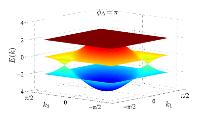
Figure 4: (Color online) Dispersion of the three bands as functions of $k_{1}$ and $k_{2}$ as defined in Eq. (5) in the kagome lattice at $\phi_{\Delta}=\pi$, i.e., $n=4$ in Eq. (8), and $\vartheta_{i}=\phi_{\Delta}/3$ and no local potentials. The hopping is set to $t=1$.

For simplicity, we choose $m_{1}=m_{2}=0$, thus $\Delta\vartheta=0$, and vary $m_{3}=n$ to achieve various fluxes $\phi_{\Delta}$. As pointed out above, one only has to consider eight values of $\phi_{\Delta}$ because of the $2\pi$-periodicity and the quantization condition (8). Additionally, $\phi_{\Delta}\to\phi_{\Delta}+\pi$ only inverts the energies and swaps Chern numbers so that it is sufficient to consider $n=0,1,2,3$. For instance, $n=4$ corresponds to adding the phase $\pi$ and, indeed, Fig. 4 displays the negative bands of Fig. 2. The degenerate, touching bands do not allow for an unambiguous definition of the Chern number. But the fact that the Hamiltonian matrix is equivalent to a real matrix up to a gauge transformation (14) teaches us that the bands are topologically trivial $C_{n}=0$.

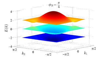
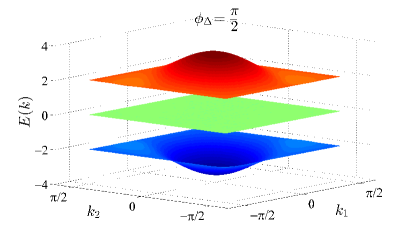
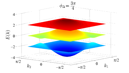
Figure 5: (Color online) Dispersion of the three bands as functions of $k_{1}$ and $k_{2}$ as defined in Eq. (5) in the kagome lattice at $\phi_{\Delta}=(\pi/4)n$ for $n=1$ (top), $n=2$ (middle), and $n=3$ (bottom) and $\vartheta_{i}=\phi_{\Delta}/3$ and no local potentials. The hopping is set to $t=1$.

The three cases $n=1,2,3$ are much more interesting; the corresponding bands are depicted in Fig. 5 in ascending order. All three bands are separated from one another so that the Chern numbers are well defined. Note the gradual evolution upon increasing flux, illustrated nicely from Fig. 2 over the panels of Fig. 5 to Fig. 4.

The fact that $\phi_{\Delta}\to\pi-\phi_{\Delta}$ inverts the signs of the energies is nicely illustrated by comparing Fig. 2 and Fig. 4. The same relation is seen between the upper and the lower panels of Fig. 5. The middle panel of Fig. 5 remains unchanged under inversion of the signs, which implies that the upper and lower bands differ only by their sign and that the middle band is identical to zero.

Next, we turn to the Chern numbers of the bands. We did not find a way to evaluate the expressions in Eqs. (1) analytically. Moreover, the two-dimensional integrals are difficult to implement numerically to high precision. But due to the robustness of the discrete Chern numbers the computation of accumulated phases on a finite mesh is very accurate, even if the mesh is not particularly dense Fukui et al. (2005). Thus we use this approach to compute the Chern numbers shown in Fig. 6.

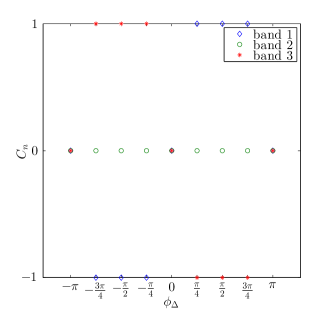
Figure 6: (Color online) Chern number $C_{n}$ as defined in Eqs. (1) computed for various fluxes $\phi_{\Delta}$ for $\vartheta_{1}=\vartheta_{2}=\phi_{\Delta}/3$. The bands are numbered in order of ascending energy.

Several interesting observations can be made. First, the fluxes, which are multiples of $\pi$, indeed yield trivial bands. Second, incrementing the flux by $\pi$ yields a swap of the Chern numbers due to the inverted global sign of the energies. The change $\phi_{\Delta}\to\pi-\phi_{\Delta}$ leaves the Chern numbers unchanged. Third, swapping the sign of the fluxes swaps also the sign of the Chern numbers. Fourth, the gradual evolution of the bands from $\phi_{\Delta}=\pi/4$ to $\phi_{\Delta}=3\pi/4$ with energetically well-separated bands is reflected in constant Chern numbers.

Further values of $\phi_{\Delta}$ do not need to be analyzed because of the $2\pi$-periodicity of the Chern numbers as a function of $\phi_{\Delta}$. Thus the pattern in Fig. 6 will occur repeatedly.

III.2 Robustness against local potentials

In order to illustrate that the Chern numbers are robust against small changes of the Hamiltonian we turn to the case with local potentials. Clearly, equal changes of all potentials $V_{A},V_{B}$, and $V_{C}$ do not affect the Chern number at all because they simply add an identity matrix to $\mathcal{H}_{\textbf{k}}$ which shifts the eigenenergy but has no impact on the eigenvectors and hence no impact on the Chern numbers; see Eqs. (1).

For illustration, we study two nontrivial patterns of the local potentials, namely $V_{A}=\delta=-V_{B}$ and $V_{C}=0$ in Fig. 7 and $V_{A}=\delta=V_{C}$ and $V_{B}=0$ in Fig. 8. These patterns are applied to the case $\phi_{\Delta}=\pi/2$ of which the dispersion without local potentials is shown in the middle panel of Fig. 5. Clearly, the nontrivial Chern numbers of the lower and upper bands are robust against the local potentials. It is necessary to apply potentials of the order of $\delta\approx t$ to destroy the topological phases because these phases are protected by gaps; see the middle panel of Fig. 5. This is numerically shown in Figs. 7 and 8 and can be analytically verified. For the pattern $V_{A}=\delta=-V_{B}$ and $V_{C}=0$, the gaps close at $|\delta|=\sqrt{2}$, and for the pattern $V_{A}=\delta=V_{C}$ and $V_{B}=0$, they close at $|\delta|={2}$.

These exemplary results illustrate the robustness of topological phases against perturbations. For the topological character to be lost the bands must touch and become degenerate. A deformation alone is not sufficient.

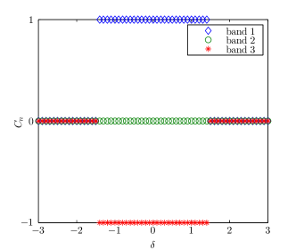
Figure 7: (Color online) Chern number $C_{n}$ as defined in Eqs. (1) computed for flux $\phi_{\Delta}=\pi/2$ for $\vartheta_{1}=\vartheta_{2}=\pi/6$ at finite local potential according to $V_{A}=\delta=-V_{B}$ and $V_{C}=0$. The hopping $t$ is set to $1$ as before.

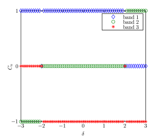
Figure 8: (Color online) Chern number $C_{n}$ as defined in Eqs. (1) computed for flux $\phi_{\Delta}=\pi/2$ for $\vartheta_{1}=\vartheta_{2}=\pi/6$ at finite local potential according to $V_{A}=\delta=V_{C}$ and $V_{B}=0$. The hopping $t$ is set to $1$ as before.

IV Edge states

For measurable quantities the bulk properties are not of prime interest. The main difference between a usual, trivial band insulator and a topological one occurs at the boundaries where states with vanishing gap have to appear since otherwise the integer Chern numbers cannot change from their finite value to zero. These edge states are crucial for the interesting properties of topologically ordered systems.

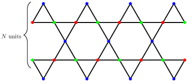
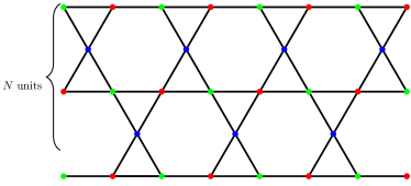
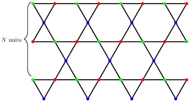
Figure 9: (Color online) Three types of edges: with triangular teeth at both edges (top), for smooth boundaries without triangular teeth at both edges (middle), and for mixed boundaries which are smooth at the upper edge and saw-toothed at the lower edge (bottom). The bracket labeled “$N$ units” stands for $N$ times repeated units between the boundaries.

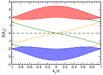
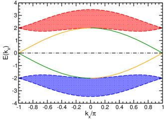
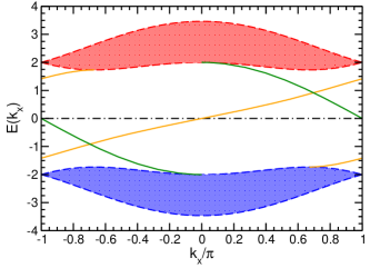
Figure 10: (Color online) Dispersions of the edge states at $\phi_{\Delta}=\pi/2$ if the edges are shaped as shown in Fig. 9: the top, middle, and bottom panels here shows the data relevant for the corresponding panel in Fig. 9. The right-moving states from the lower edge are shown in orange and the left-moving ones from the upper edge in dark green. The shaded area stands for the continua of the bulk states if $k_{y}$ is not fixed. The dashed line at zero stands for the nondispersive bulk states of the trivial middle band; cf. middle panel in Fig. 5.

To illustrate the existence of such edge states also in the kagome lattice in a magnetic field we diagonalize strips of it. A strip is infinitely extended in the $x$ direction such that $k_{x}$ is a conserved quantum numbers. But in the $y$ direction the strip is of finite extension. Three different situations of the boundaries are displayed in Fig. 9. The height of the strips is fixed by the number $N$ of repeated units of six sites in the perpendicular $y$ direction. The dispersions of the in-gap edges states converge very quickly for $N\to\infty$. Our results are based on computations with $N=80$ which amounts to the diagonalization of matrices of dimension 480.

The resulting dispersions are shown in Fig. 10. Strikingly, there occur significant differences for the dispersions of the differently shaped boundaries. Even the group velocities differ by about a factor of 2.

These differences make the assignment of the edge states to the upper and lower edges particularly simple by analyzing mixed boundaries; see the lower panels in Figs. 9 and 10. Clearly, we partly find the dispersion from the upper panel for the right-moving states and from the lower panel for the left-moving states. Thus the right-moving states live at the lower edge and the left-moving states at the upper edge. Of course, this will be swapped if the sign of the magnetic field is inverted.

We conclude that the shapes of the boundaries open an interesting field for tuning the properties, for instance the transport properties, of topologically nontrivial bands.

V Conclusions

We have shown that a crystal lattice with basis equally allows us to induce topologically nontrivial bands upon application of a uniform magnetic field. Interestingly, the number of bands does not need to be increased from the values at zero magnetic field, which is in contrast to the situation in Bravais lattices Hofstadter (1976); Aidelsburger et al. (2015).

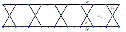
Figure 11: (Color online) Phases after the gauge transformation $c_{i}^{\dagger}\to c_{i}^{\dagger}\exp(\mp\mathrm{i}\vartheta)$ for A and B sites, respectively. The experimental realization should be easier in this gauge.

In particular, we studied nearest-neighbor hopping on the kagome lattice with a three-fold basis. This lattice is made of triangular loops, i.e., loops with the smallest number of odd bonds which generically induces frustration effects. Without magnetic field the bands are not separated, but the special magnetic fields which preserve the commutation of the translations induce a proper splitting and nonzero Chern numbers for two of the three bands. Interestingly, we found that the kagome lattice in a uniform magnetic field of particular strengths realizes Haldane models on this lattice for particular quantized fluxes.

It would be interesting to realize crystal lattices with nontrivial gauges experimentally Jiménez-García et al. (2012); Aidelsburger et al. (2015). In order not to be forced to induce finite phases $\vartheta:=\vartheta_{1}=\vartheta_{2}$ for all hopping processes, we point out that a simple gauge transformation eliminates all phases on bonds to or from sites of the sublattice C. It consists of the additional factor $c_{i}^{\dagger}\to c_{i}^{\dagger}\exp(-i\vartheta)$ for A sites and the additional factor $c_{i}^{\dagger}\to c_{i}^{\dagger}\exp(i\vartheta)$ for B sites. Of course, the fluxes through the triangles are left unchanged because the phases on bonds between the A and B sites are tripled, $\vartheta\to 3\vartheta$, as shown in Fig. 11.

Finally, we investigated the edge states for three ways to cut the kagome lattice along the same direction. Again, this possibility is a particular feature for lattices with a basis. Surprisingly, we found a significant qualitative dependence of the dispersion of the edge states on the nature of the boundaries. The shape and the position of the dispersions differ as well as the group velocities. Still there are left- and right-moving modes which can be clearly assigned to the upper or lower edge. The situation is particularly clear if the upper and lower edges differ. Then we obtained two differing edge states, one reflecting the behavior at the upper edge and one the behavior at the lower edge.

Experimental verification of this interesting scenario is called for. One may envisage fascinating applications because the transport properties will differ depending on the direction of motion of a fermion from left to right or vice versa. It is conceivable to build diode like devices if the properties of the edges are tuned to maximize their differing characteristics, for instance the group velocity.

At present, the most promising systems for experimental realization are not yet clear Bergholtz and Liu (2013). But recent advances in realizing artificial gauges in systems of optical lattices Jiménez-García et al. (2012); Aidelsburger et al. (2015); Jotzu et al. (2014) make it likely that soon the theoretical results presented here can be put to experimental tests. The realization of precisely defined edges may pose a problem, but any reproducible difference between two edges of a strip of lattice will make a verification possible.

Alternatively, various solid-state systems may constitute alternative routes towards experimental realizations, for instance thin slabs of ferromagnetic Chern insulators Chang et al. (2013); Kou et al. (2014); Chang et al. (2015), honeycomb lattices built from atoms with higher atomic number Wu et al. (2014), artificial lattices on surfaces Krasheninnikov and Nieminen (2011); Han et al. (2015), or special lattices built from semiconductor nanostructures Lan and Ding (2012). In any case, we conclude that designed crystal lattices constitute a promising field of research.

Appendix A Arbitrary magnetic flux

In Fig. 12 a general gauge is shown which is a lattice version of the Landau gauge. The phases depend on the $x$ coordinate of their bond, i.e., on the $x$ coordinate of the midpoint of their bond. The dependence is linear,

$$\varphi(x):=4\phi_{\Delta}x,$$ (18)

where we imply that the lattice constant is set to unity.

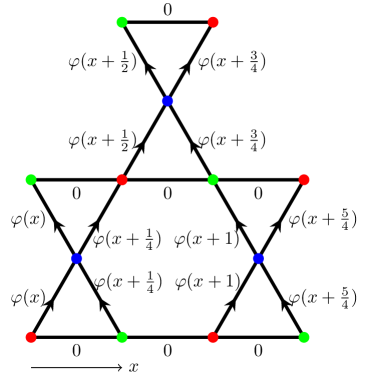
Figure 12: (Color online) Gauge for arbitrary magnetic flux, i.e., for arbitrary homogeneous magnetic field. Recall that the lattice constant, i.e., double the distance between neighboring sites, is set to unity.

Then it is easy to see that indeed the flux through a triangle is given by

$$\phi_{\Delta}=\varphi(x+\frac{1}{4})-\varphi(x)$$ (19)

so that our notation is consistent. Similarly, we find for the flux through the hexagon

$$\phi_{\mathrm{hexagon}} = 2\varphi(x+1)-2\varphi(x+\frac{1}{4})$$ (20a)

$$= 6\phi_{\Delta}$$ (20b)

as it has to be for a homogeneous magnetic field. In total, the flux through a unit cell is given by $8\phi_{\Delta}$. Note that these results do not change if we consider shifted triangles or hexagons in other parts of the lattice. Shifts in the $y$ direction do not change the phases (18) at all. Shifts in the $x$ direction do not change the fluxes because they depend on phase differences being independent of $x$ due to the linearity of Eq. (18). So the gauge shown in Fig. 12 correctly describes the effect of an arbitrary homogeneous magnetic field perpendicular to the plane of the lattice.

Appendix B Translational invariant gauge for specific magnetic fluxes

Here we show that for $\phi_{\Delta}=n\pi/4$ the gauge in Fig. 12 can be regauged to yield the gauge in Fig. 13. For clarity we focus on the case $\vartheta_{1}=\vartheta_{2}=\phi_{\Delta}/3$, i.e., $m_{1}=m_{2}=0$ in Eq. (9).

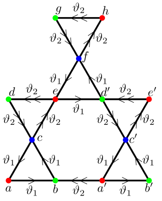
Figure 13: (Color online) Gauge for specific magnetic fluxes, i.e., for specific homogeneous magnetic fields. The necessary regauging on the various sites $a$ to $h$ and $a^{\prime}$ to $e^{\prime}$ are given in the main text.

We leave the fermion at site $a$ in Fig. 13 unchanged, but we transform the others according to

$$c^{\dagger}_{a} \to c^{\dagger}_{a},$$ (21a)

$$c^{\dagger}_{b} \to c^{\dagger}_{b}\exp(i\vartheta_{1}),$$ (21b)

$$c^{\dagger}_{c} \to c^{\dagger}_{c}\exp(2i\vartheta_{1}-i\varphi(x+1/4)),$$ (21c)

$$c^{\dagger}_{e} \to c^{\dagger}_{e}\exp(3i\vartheta_{1}-i2\varphi(x+1/4)),$$ (21d)

$$c^{\dagger}_{d} \to c^{\dagger}_{d}\exp(i\vartheta_{1}-i\varphi(x)-i\varphi(x+1/4)).$$ (21e)

The annihilation operators are transformed by the complex conjugate phase factors. Obviously, the phase factors are chosen such that the phases on the bonds $ab$, $bc$, $ce$, and $cd$ match those in Fig. 13. We have to check the resulting phase factor on $ca$ and compute

$$\vartheta_{ca} = -2\vartheta_{1}+\varphi(x+1/4)-\varphi(x)$$ (22a)

$$= -(2/3)\phi_{\Delta}+\phi_{\Delta}$$ (22b)

$$= \phi_{\Delta}/3$$ (22c)

$$= \vartheta_{1},$$ (22d)

which is what we wanted to have. Analogously, we confirm for the phase on bond $ed$

$$\vartheta_{ed} = \vartheta_{1}-\varphi(x)-3\vartheta_{1}+\varphi(x+1/4)$$ (23a)

$$= -(2/3)\phi_{\Delta}+\phi_{\Delta}$$ (23b)

$$= \phi_{\Delta}/3$$ (23c)

$$= \vartheta_{2}.$$ (23d)

If we now pass from the sites $a$ to $e$ to the sites $a^{\prime}$ to $e^{\prime}$ we can use almost the same transformations (21) because the phases on the bonds are changed by multiples of $\pi$ due to

$$\phi(\tilde{x}+1) = \phi(\tilde{x})+4\phi_{\Delta}$$ (24a)

$$= \phi(\tilde{x})+n\pi$$ (24b)

for any $\tilde{x}$. This is so because $\phi_{\Delta}$ takes the particular values $n\pi/4$ representing the crucial step in our argument.

If $n$ is even we may use exactly the same transformations. If $n$ is odd we regauge the center site $c^{\prime}$ by the factor $-1$ and we are back to the phases between the sites $a$ through $e$ and use the regauge transformation (21). In addition, it is obvious that the phases on the bonds $ba^{\prime}$ and $ed^{\prime}$ correspond to the ones in Fig. 13.

For completeness, we state the regauge transformations on sites $f$, $g$, and $h$,

$$c^{\dagger}_{f} \to c^{\dagger}_{f}\exp(2i\vartheta_{1}-3i\varphi(x)-4i\phi_{\Delta}),$$ (25a)

$$c^{\dagger}_{g} \to c^{\dagger}_{g}\exp(i\vartheta_{1}-4i\varphi(x)-6i\phi_{\Delta}),$$ (25b)

$$c^{\dagger}_{h} \to c^{\dagger}_{h}\exp(3i\vartheta_{1}-4i\varphi(x)-7i\phi_{\Delta}),$$ (25c)

because they are not directly deduced from the ones on $a$ to $e$. Straightforward calculations verify that these transforms yield the phase pattern shown in Fig. 13. The sites resulting from a shift by one lattice constant to the right are again transformed either exactly the same way as the sites $e$ to $h$ and $d^{\prime}$ if $n$ is even. For odd $n$, the same transformations are used except for an additional sign change on the shifted center site $f^{\prime}$.

In the next upper row the phase pattern for the row of sites $a$ to $e$ is repeated. Thus one can reuse the transformations (21) except that all the phases must be taken relative to the phase of the $h$ site [Eq. (25c)].

In an analogous fashion, one can implement regauge transformations yielding $\vartheta_{1}\neq\vartheta_{2}$, but they are slightly more complex because they comprise a certain phase shift upon $x\to x+1$.

In conclusion, we can regauge the case of a general homogeneous magnetic field to the phases shown in Figs. 3 or 13.

References

- v. Klitzing et al. (1980) K. v. Klitzing, G. Dorda, and M. Pepper, Phys. Rev. Lett. 45, 494 (1980).
- Tsui et al. (1982) D. C. Tsui, H. L. Stormer, and A. C. Gossard, Phys. Rev. Lett. 48, 1559 (1982).
- Berry (1984) M. V. Berry, Phys. Roy. Soc. Lond. A 392, 45 (1984).
- Niu et al. (1985) Q. Niu, D. J. Thouless, and Y.-S. Wu, Phys. Rev. B 31, 3372 (1985).
- Wegner (1988) F. J. Wegner, Publication de l’Institut de Recherche Mathématique Avancée 39, 21 (1988).
- Klein and Seiler (1990) M. Klein and R. Seiler, Commun. Math. Phys. 128, 141 (1990).
- Uhrig (1991) G. S. Uhrig, Z. Phys. B 82, 29 (1991).
- Ando (2013) Y. Ando, J. Phys. Soc. Jpn. 82, 102001 (2013).
- Süsstrunk and Huber (2015) R. Süsstrunk and S. D. Huber, Science 349, 47 (2015).
- Jiménez-García et al. (2012) K. Jiménez-García, L. J. LeBlanc, R. A. Williams, M. C. Beeler, A. R. Perry, and I. B. Spielman, Phys. Rev. Lett. 108, 225303 (2012).
- Aidelsburger et al. (2015) M. Aidelsburger, M. Lohse, C. Schweizer, M. Atala, J. T. Barreiro, S. Nascimbène, N. R. Cooper, I. Bloch, and N. Goldman, Nature Phys. 11, 162 (2015).
- Romhányi et al. (2015) J. Romhányi, K. Penc, and R. Ganesh, Nature Comm. 6, 6805 (2015).
- Jotzu et al. (2014) G. Jotzu, M. Messer, R. Desbuquois, M. Lebrat, T. Uehlinger, D. Greif, and T. Esslinger, Nature 515, 237 (2014).
- Chang et al. (2013) C.-Z. Chang, J. Zhang, X. Feng, J. Shen, Z. Zhang, M. Guo, K. Li, Y. Ou, P. Wei, L.-L. Wang, et al., Science 340, 167 (2013).
- Kou et al. (2014) X. Kou, S.-T. Guo, Y. Fan, L. Pan, M. Lang, Y. Jiang, Q. Shao, T. Nie, K. Murata, J. Tang, et al., Phys. Rev. Lett. 113, 137201 (2014).
- Chang et al. (2015) C.-Z. Chang, W. Zhao, D. Y. Kim, H. Zhang, B. A. Assaf, D. Heiman, S.-C. Zhang, C. Liu, M. H. W. Chan, and J. S. Moodera, Nature Mat. 14, 473 (2015).
- Wu et al. (2014) S.-C. Wu, G. Shan, and B. Yan, Phys. Rev. Lett. 113, 256401 (2014).
- Han et al. (2015) Y. Han, J.-G. Wan, G.-X. Ge, F.-Q. Song, and G.-H. Wang, Sci. Rep. 5, 16843 (2015).
- Krasheninnikov and Nieminen (2011) A. V. Krasheninnikov and R. M. Nieminen, Theor. Chem. Acc 129, 625 (2011).
- Lan and Ding (2012) H. Lan and Y. Ding, Nano Today 7, 94 (2012).
- Haldane (1988) F. D. M. Haldane, Phys. Rev. Lett. 61, 2015 (1988).
- Ohgushi et al. (2000) K. Ohgushi, S. Murakami, and N. Nagaosa, Phys. Rev. B 62, R6065 (2000).
- Katsura et al. (2010) H. Katsura, N. Nagaosa, and P. A. Lee, Phys. Rev. Lett. 104, 066403 (2010).
- Tang et al. (2011) E. Tang, J.-W. Mei, and X.-G. Wen, Phys. Rev. Lett. 106, 236802 (2011).
- Bergholtz and Liu (2013) E. J. Bergholtz and Z. Liu, Int. J. Mod. Phys. B 27, 1330017 (2013).
- Mielke (1991a) A. Mielke, J. Phys. A 24, L73 (1991a).
- Mielke (1991b) A. Mielke, J. Phys. A24, 3311 (1991b).
- Zak (1964a) J. Zak, Phys. Rev. 134, A1602 (1964a).
- Zak (1964b) J. Zak, Phys. Rev. 136, A1647 (1964b).
- Kohmoto (1985) M. Kohmoto, Ann. of Phys. 160, 343 (1985).
- Hofstadter (1976) D. R. Hofstadter, Phys. Rev. B 14, 2239 (1976).
- Fukui et al. (2005) T. Fukui, Y. Hatsugai, and H. Suzuki, J. Phys. Soc. Jpn. 74, 1674 (2005).