Rank-1 Tensor Approximation Methods
and Application to Deflation

Abstract

Because of the attractiveness of the canonical polyadic (CP) tensor decomposition in various applications, several algorithms have been designed to compute it, but efficient ones are still lacking. Iterative deflation algorithms based on successive rank-1 approximations can be used to perform this task, since the latter are rather easy to compute. We first present an algebraic rank-1 approximation method that performs better than the standard higher-order singular value decomposition (HOSVD) for three-way tensors. Second, we propose a new iterative rank-1 approximation algorithm that improves any other rank-1 approximation method. Third, we describe a probabilistic framework allowing to study the convergence of deflation CP decomposition (DCPD) algorithms based on successive rank-1 approximations. A set of computer experiments then validates theoretical results and demonstrates the efficiency of DCPD algorithms compared to other ones.

I Introduction

In the last years, tensors have been playing an important role in many applications such as blind source separation [1, 2], telecommunications [3], chemometrics [4], neuroscience [5], sensor array processing [6] and data mining [7]. The attractiveness behind tensors lies in the uniqueness of their canonical polyadic (CP) decomposition under mild conditions [8], which is a powerful property not shared by standard matrix-based tools. There are several methods to compute the CP tensor decomposition. We will point out here some of the most used methods among many others. For the exact CP decomposition, [9] proposes a direct computation to decompose $2\times n\times n$ tensors. In [10], a generalization of Sylvester’s algorithm is described for decomposing symmetric tensors. In [11], one can use simultaneous matrix diagonalization by congruence, provided that the rank of the tensor is smaller than its greatest dimension. An approach based on eigenvectors of tensors is proposed in [12].

In practice, tensors are corrupted by noise so that one needs to compute an approximate decomposition of given rank. Computing the exact CP decomposition is difficult [13], but finding a lower-rank approximation is even harder. In fact, this is an ill-posed problem in general [14]. Nevertheless, some useful algorithms have been conceived to solve locally the low-rank approximation problem. This kind of algorithms can be found in [15, 16, 17, 18, 19]. One of the most widely used is the alternating least squares (ALS) algorithm [4], which is an iterative method that consists in conditionally updating in an alternate way, the matrix factors composing the CP decomposition. Other gradient and Newton-based methods estimate the factor matrices all-at-once. Howsoever, all theses algorithms have disappointing convergence properties [15, 20]. Another kind of algorithms is based on rank-1 deflation. It is known that the conventional deflation works for matrices but not for tensors [21]. In [22], the authors propose deflation methods that work only if the rank of the tensor is not larger than its dimensions. In [23], ALS is used to update the columns of matrix factors in a deflation procedure, but for non-negative tensors. However, these deflation methods strongly depend on initialization and no convergence study has been conducted.

In the same vein of iterative deflation, the authors proposed in [24] a deflation-based CP decomposition (DCPD), based on successive rank-1 approximations computed by low-complexity methods. Other rank-1 approximation methods can be used in DCPD, for instance, ALS. However, the latter exhibits an unbounded complexity and no satisfactory convergence study is available for rank-1 approximation apart [26], which shows results on the global convergence for generic tensors in the sense that, for any initialization, ALS converges to the same point in general. A quasi-Newton method defined on Grassmannians are developed in [27]. However, they exhibit an unbounded complexity to compute rank-1 approximations, since these methods need to be iterated. In [28], the best rank-1 approximation problem can be computed by means of an algebraic geometry moment method, but it is only applicable to very small tensor dimensions since the number of variables grows exponentially when building convex relaxations. Moreover, even for small dimensions, its convergence is very slow. In [29], the authors propose an improvement method for [28] based on border basis relaxation, but again the method is limited to small tensor dimensions. Semidefinite relaxations are proposed in [30] to compute rank-1 approximations, however the convergence becomes very slow when dimensions are large.

In this paper, we report mainly three contributions. First, we propose an algebraic rank-1 approximation method, namely the sequential rank-1 approximation and projection (SeROAP), which can perform better than the standard truncated high-order singular value decomposition (THOSVD) [25]. Indeed, we prove that the rank-1 approximation performed by SeROAP is always better than the one obtained from THSOVD for three-way tensors. Moreover, for large dimensions and small orders, we show that the computational complexity of SeROAP is dramatically lower than that of THOSVD.

Second, we propose an alternating eigenvalue rank-1 iterative algorithm for three-way tensors, namely CE (coupled-eigenvalue), that improves other rank-1 approximation algorithms. We prove that if the solution obtained from some rank-1 approximation algorithm (e.g., SeROAP, THOSVD) is the input of the CE algorithm, the performed rank-1 approximation remains the same in the worst case. We also prove that the convergence to a stationary point is always guaranteed. Actually, results have shown that when the initialization of the CE algorithm is close enough to the global solution, it recovers the best rank-1 approximation. Furthermore, when one dimension is much larger than the other two dimensions, the computational complexity of the CE algorithm can be lower than that of the standard ALS algorithm.

Third, we perform a theoretical study on deflation in order to analyze the convergence of the DCPD algorithm. In a first stage, we show that the norm of residuals is monotonically reduced within the iterative deflation process. We also prove that the DCPD algorithm recovers the exact CP decomposition of a given tensor when residuals do not fall within a cone with an arbitrary small volume. In a second stage, we prove that the iterative deflation method can reduce the norm of the initial residual by a factor smaller than $\left(\sin(\beta)\right)^{L-1}$ ($\beta$ being the angle of a suitable cone where the residuals can fall in) after $L$ iterations with high probability, when tensors are distributed according to an absolutely continuous probability measure, and the probability function of residuals is continuous on some suitable angular interval. We also present a conjecture stating the existence of probability measures ensuring the convergence of the DCPD algorithm to an exact decomposition with high probability.

The paper is organized as follows. In Section III some standard iterative methods and the DCPD algorithm as well as SeROAP and THOSVD methods are described. The computational complexity per iteration for each algorithm is provided. The next two sections form the core of the paper. In Section IV, we first prove that SeROAP performs better than THOSVD as far as rank-1 approximations of three-way tensors is concerned. Then in a second part, the CE algorithm is presented as well as the proof that it can refine any other rank-1 approximation method and the proof of its convergence. In Section V, among other theoretical results, we study conditions ensuring the convergence of the DCPD algorithm. Finally, in Section VI, computer results show satisfactory performances of the proposed DCPD and rank-1 approximation methods, compared to other related algorithms, even under noisy scenarios.

II Notation

The notation employed in this paper is the following. Scalar numbers are denoted by lowercase letters and vectors by boldface lowercase ones. For matrices and tensors, boldface capital and calligraphic letters are used, respectively. Plain capitals are used to denote array dimensions. Depending on the context, greek letters can denote either scalars, vectors, matrices or tensors. The symbols $\boxdot,\odot,\boxtimes$ and $\otimes$ denote the Hadamard, Khatri-Rao, Kronecker and tensorial products, respectively, and ⁺ denotes matrix pseudo-inversion. The Euclidean scalar product between tensors is denoted by $\langle\boldsymbol{\mathcal{T}},\boldsymbol{\mathcal{U}}\rangle=\sum_{i_{1}\cdots i_{N}}T_{i_{1}\cdots i_{N}}U^{*}_{i_{1}\cdots i_{N}}$. The angle between two tensors $\boldsymbol{\mathcal{U}}$ and $\boldsymbol{\mathcal{V}}$ will refer to $\arccos\{|\langle\boldsymbol{\mathcal{U}},\boldsymbol{\mathcal{V}}\rangle|\}/\|\boldsymbol{\mathcal{U}}\|_{F}\,\|\boldsymbol{\mathcal{V}}\|_{F}\in[0,\,\pi/2]$. $\|\cdot\|$ then denotes the Frobenius norm induced by the previous scalar product. We shall also use the $\ell^{2}$ operator norm $\|\cdot\|_{2}$ for matrices, which corresponds to the largest singular value. The mode-$n$ unfolding of a tensor $\boldsymbol{\mathcal{T}}$ is denoted as $\boldsymbol{T}_{(n)}$, as proposed in [16]. $\boldsymbol{\mathcal{T}}(:,j,k)$, $\boldsymbol{\mathcal{T}}(i,:,k)$ and $\boldsymbol{\mathcal{T}}(i,j,:)$ denote vector slices of tensor $\boldsymbol{\mathcal{T}}$.

The operator $\mathop{\operator@font vec}$ is the vectorization operator that stacks the columns of a matrix into a long column vector, and $\mathop{\operator@font Unvec}$ is its reverse operator. $C^{k}$ is the set of functions having continuous $k$th derivatives. Finally, $\mathbb{K}$ is either the real or the complex field.

III Description of Algorithms and Complexity Analysis

This section presents the description of some CP decomposition algorithms. In order to support further results, the complexity per iteration is calculated here for each algorithm using Landau’s notation, denoted by $\mathcal{O}$, and counting only multiplications, as recommended in [31]. From Section III-A to Section III-B, we describe two classical algorithms known in literature: ALS and conjugate gradient [15]. In Section III-C, the DCPD algorithm is presented.

For the CP decomposition algorithms described in the following, the input parameter $R$ denotes the rank of the output tensor. Assuming $R_{0}$ is the rank of the input tensor $\boldsymbol{\mathcal{T}}$, if $R_{0}\leq R$, then the algorithms perform an exact decomposition. On the other hand, if $R_{0}>R$, a lower rank-$R$ approximation is computed.

III-A Alternating least squares (ALS)

The most commonly used algorithm for solving the CP decomposition is ALS [4]. The goal is to update alternately each factor matrix in each iteration by solving a least squares problem conditioned on previous updates of the other factor matrices. There is no guarantee of convergence to the global solution, nor even to a critical point. The implementation is quite simple and it is detailed in Alg.1.

input : $\boldsymbol{\mathcal{T}}\in\mbox{$\mathbb{K}$}^{I_{1}\times I_{2}\times\cdots\times I_{N}}$: input data,

R: rank parameter.

output : $\boldsymbol{A}^{(n)}\in\mbox{$\mathbb{K}$}^{I_{n}\times R}$, for $n=1,\ldots,N$: factor matrices

Initialize $\boldsymbol{A}^{(1)},\ldots,\boldsymbol{A}^{(N)}$

repeat

       for $n=1$ to $N$ do

             $\boldsymbol{V}\leftarrow\boldsymbol{A}^{(1){\sf T}}\boldsymbol{A}^{(1)}\boxdot\cdots\boxdot\boldsymbol{A}^{(n-1){\sf T}}\boldsymbol{A}^{(n-1)}\boxdot\boldsymbol{A}^{(n+1){\sf T}}\boldsymbol{A}^{(n+1)}\boxdot\cdots\boxdot\boldsymbol{A}^{(N){\sf T}}\boldsymbol{A}^{(N)}$

            $\boldsymbol{A}^{(n)}=\boldsymbol{T}_{(n)}(\boldsymbol{A}^{(N)}\odot\cdots\odot\boldsymbol{A}^{(n+1)}\odot\boldsymbol{A}^{(n-1)}\odot\cdots\odot\boldsymbol{A}^{(1)})\boldsymbol{V}^{+}$

       end for

      

until some stopping criterion is satisfied;

Algorithm 1 ALS algorithm

The complexity per iteration (repeat loop) of ALS may be calculated as follows. The computation of matrix $\boldsymbol{V}$ needs $(I_{1}+\ldots+I_{n-1}+I_{n+1}\ldots I_{N})R^{2}+(N-2)R^{2}$ operations (multiplications). The pseudo-inverse of $\boldsymbol{V}$ is calculated by resorting to an SVD. For a $m\times n$ rank-$r$ matrix, with $m\geq n\geq r$, the explicit calculation of diagonal, left singular, and right singular matrices require $2mn^{2}-2n^{3}/3,5mr^{2}-r^{3}/3,$ and $5nr^{2}-r^{3}/3$ multiplications, respectively [31]. Thus, assuming for simplicity that $\boldsymbol{V}$ is a non-singular matrix, the number of operations to calculate its pseudo inverse is $35R^{3}/3+R^{2}$. For updating $\boldsymbol{A}^{(n)}$, we need

$$R\!\!\prod_{i=1,i\neq n}^{N}\!\!\!I_{i}+R\prod_{j=1}^{N}I_{j}+I_{n}R^{2}$$

multiplications. These calculations must be performed for each $n\in\{1,\ldots,N\}$. Thus, the number of operations per iteration for ALS is dominated by the term composed of the product of all dimensions. Hence,

$$\#op=\mathcal{O}\bigg{\{}NR\prod\limits_{j=1}^{N}I_{j}\bigg{\}}.$$ (1)

III-B Conjugate gradient (CG)

The conjugate gradient algorithm (CG) is a faster algorithm than the well known gradient descent [15]. Here, we use the optimum step size and the Polak-Ribière implementation [32] for updating the parameter $\beta$ in the algorithm presented in Alg.2. The number of operations for computing each vector $\boldsymbol{g}_{n}$ is

$$R^{2}\sum\limits_{j=1}^{N}I_{j}+(N-2)R^{2}+I_{n}R^{2}+R\!\!\prod\limits_{i=1,i\neq n}^{N}\!\!\!I_{i}+R\prod\limits_{j=1}^{N}I_{j}$$

The computation of the step size $\mu^{\star}$ is dominated by the number of multiplications needed to determine all the coefficients but one of a $2N$-degree polynomial generated from the enhanced line search (ELS) method, which is given by [17]:

$$\left(2^{N}R+\mathcal{O}\{N^{2}\}\right)\prod\limits_{j=1}^{N}I_{j}$$

input : $\boldsymbol{\mathcal{T}}\in\mbox{$\mathbb{K}$}^{I_{1}\times I_{2}\times\cdots\times I_{N}}$: input data,

R: rank parameter.

output : $\boldsymbol{A}^{(n)}\in\mbox{$\mathbb{K}$}^{I_{n}\times R}$, for $n=1,\ldots,N$: factor matrices

Initialize $\boldsymbol{A}^{(1)},\ldots,\boldsymbol{A}^{(N)}$;

$\boldsymbol{p}\leftarrow[vec^{{\sf T}}(\boldsymbol{A}^{(1)})\cdots vec^{{\sf T}}(\boldsymbol{A}^{(N)})]^{{\sf T}}$;

repeat

      

      for $n=1$ to $N$ do

            

            Compute the gradient $\boldsymbol{g}_{(n)}$ with respect $vec(\boldsymbol{A}^{(n)})$;

       end for

      

      $\boldsymbol{g}\leftarrow[\boldsymbol{g}^{{\sf T}}_{(1)}\ldots\boldsymbol{g}^{{\sf T}}_{(N)}]^{{\sf T}}$;

      if $n=1$ then

             $\boldsymbol{d}\leftarrow-\boldsymbol{g}$;

       end if

      

      Compute the optimum step size $\mu^{\star}$;

      Update $\beta$ according to Polak-Ribière;

      $\Delta\boldsymbol{p}\leftarrow\mu^{\star}\boldsymbol{d}$;

      $\boldsymbol{p}\leftarrow\boldsymbol{p}+\Delta\boldsymbol{p}$;

      $\boldsymbol{d}\leftarrow-\boldsymbol{g}+\beta\boldsymbol{d}$;

until some stopping criterion is satisfied;

Extract $\boldsymbol{A}^{(n)}$ from $\boldsymbol{p}$, for $n=1,\dots,N.$

Algorithm 2 CG algorithm

The parameter $\beta$ requires only $1+2R\sum_{j=1}^{N}I_{j}$ multiplications. Hence, the CG algorithm with ELS has a total complexity given by

$$\#op=\mathcal{O}\bigg{\{}\left((2^{N}+1)R+N^{2}\right)\prod\limits_{j=1}^{N}I_{j}\bigg{\}}.$$ (2)

III-C Deflation-based CP decomposition (DCPD)

The computation of a rank-1 approximation is the key of the DCPD algorithm. We present here two methods for computing a rank-1 approximation referred to as THOSVD and SeROAP [24].

III-C1 Truncation of higher order singular value decomposition - THOSVD

The algorithm is described in Alg.3. For computing the first right singular vector, we do not need compute the complete SVD. According to [33], we can compute the best rank-1 approximation of a $m\times n$ matrix in $k$ steps by using the Lanczos algorithm, with a complexity $\mathcal{O}\{2kmn\}$. Hence, the accumulated complexity computed for all $\boldsymbol{u}_{n}$ is equal to $\mathcal{O}\{2Nk\prod_{j=1}^{N}I_{j}\}$. The computation of $\boldsymbol{\mathcal{U}}$ requires $\prod_{j=1}^{N}I_{j}$ flops. The contraction to obtain $\lambda$ also needs $\prod_{j=1}^{N}I_{j}$ operations. To sum up, the total number of operations of THOSVD is of order:

$$\mathcal{O}\bigg{\{}(2Nk+2)\prod_{j=1}^{N}I_{j}\bigg{\}}$$

input : $\boldsymbol{\mathcal{T}}\in\mbox{$\mathbb{K}$}^{I_{1}\times I_{2}\times\cdots\times I_{N}}$: input data

output :  $\boldsymbol{\mathcal{X}}\in\mbox{$\mathbb{K}$}^{I_{1}\times I_{2}\times\cdots\times I_{N}}$: rank-1 approximation

for $n=1$ to $N$ do

      

      $\boldsymbol{u}_{n}\leftarrow$ first left singular vector of $\boldsymbol{T}_{(n)}$ ;

end for

$\boldsymbol{\mathcal{U}}\leftarrow\otimes_{n=1}^{N}\boldsymbol{u}_{n}$;

$\lambda\leftarrow\langle\boldsymbol{\mathcal{T}},\boldsymbol{\mathcal{U}}\rangle$;

$\boldsymbol{\mathcal{X}}\leftarrow\lambda\cdot\boldsymbol{\mathcal{U}}$.

Algorithm 3 THOSVD algorithm

III-C2 Sequential rank-1 approximation and projection - SeROAP

Without loss of generality, consider $I_{1}\geq I_{2}\geq\ldots\geq I_{N}$. The SeROAP algorithm [24] goes along the lines depicted in Alg.4. In the first for loop, we compute $N-2$ right singular vectors of matrices whose size is successively reduced. For this step, the complexity is $\mathcal{O}\{2k\sum_{i=1}^{N-2}(\prod_{j=i}^{N}I_{j})\}$. The computation of vectors $\boldsymbol{u},\boldsymbol{v}$ and $\boldsymbol{w}$ has complexity $\mathcal{O}\{(2k+1)I_{N-1}I_{N}\}$.

Next, the second for loop performs $N-2$ successive projections of the rows of matrices $\boldsymbol{V}_{n}$ onto the vectors $\boldsymbol{w}$. We need here $2\sum_{i=1}^{N-2}(\prod_{j=i}^{N}I_{j})$ operations.

input : $\boldsymbol{\mathcal{T}}\in\mbox{$\mathbb{K}$}^{I_{1}\times I_{2}\times\cdots\times I_{N}}$: input data

output : $\boldsymbol{\mathcal{X}}\in\mbox{$\mathbb{K}$}^{I_{1}\times I_{2}\times\cdots\times I_{N}}$: rank-1 approximation

$\boldsymbol{V}_{0}\leftarrow\boldsymbol{T}_{(1)}$;

$\boldsymbol{V}\leftarrow\boldsymbol{V}_{0}$;

for $n=1$ to $N-2$ do

      

      $\boldsymbol{v}_{n}\leftarrow$ first right singular vector of $\boldsymbol{V}$;

      $\boldsymbol{V}_{n}\leftarrow Unvec(\boldsymbol{v}_{n})\in\mbox{$\mathbb{K}$}^{I_{n+1}\times I_{n+2}I_{n+3}\cdots I_{N}}$;

      $\boldsymbol{V}\leftarrow\boldsymbol{V}_{n}$;

end for

$(\boldsymbol{u},\boldsymbol{v})\leftarrow$ first left and right singular vectors of $\boldsymbol{V}$; $\boldsymbol{w}\leftarrow\boldsymbol{v}^{*}\boxtimes\boldsymbol{u}$;

for $n=N-2$ to $1$ do

       $\boldsymbol{X}_{(n)}\leftarrow\left(\boldsymbol{V}_{n-1}\boldsymbol{w}\right)\boldsymbol{w}^{H}$;

      $\boldsymbol{w}=vec({\boldsymbol{X}_{(n)}})$;

end for

$\boldsymbol{X}_{(1)}$ is the mode-$1$ unfolding of $\boldsymbol{\mathcal{X}}$.

Algorithm 4 SeROAP algorithm

For large dimensions and small $N$, the complexity of SeROAP is dominated by:

$$\mathcal{O}\bigg{\{}(2k+2)\prod\limits_{j=1}^{N}I_{j}\bigg{\}}$$

which can be significantly smaller than that of THOSVD. An example of typical execution is given in the Appendix.

III-C3 Description and complexity of DCPD

The DCPD is an iterative deflation algorithm [24] that computes the CP decomposition for real or complex tensors. As summarized in Alg.5, it proceeds as follows. In the first for loop, we compute the rank-1 tensors $\boldsymbol{\mathcal{X}}[1,1],\ldots,\boldsymbol{\mathcal{X}}[R,1]$ by successive rank-1 approximations and subtractions. Since the rank of the tensor does not decrease with subtractions in general [21], a residual $\boldsymbol{\mathcal{E}}[R,1]$ is then produced. In the iterative process (repeat loop), a new rank-1 component is generated from the sum of the previous residual and $\boldsymbol{\mathcal{X}}[1,1]$, and a new residual $\boldsymbol{\mathcal{E}}[1,2]$ is produced with the subtraction $\boldsymbol{\mathcal{Y}}[1,2]-\boldsymbol{\mathcal{X}}[1,1]$. The tensor $\boldsymbol{\mathcal{Y}}[1,2]$ is updated within the if-else condition. By applying the same procedure to the other components, we update all $R$ rank-1 tensors, so that another residual $\boldsymbol{\mathcal{E}}[R,2]$ is generated in the end of the second for loop. The second loop continues to execute until some stopping criterion is satisfied, and all rank-1 components of $\boldsymbol{\mathcal{T}}$ can be recovered.

input : $\boldsymbol{\mathcal{T}}\in\mbox{$\mathbb{K}$}^{I_{1}\times I_{2}\times\cdots\times I_{N}}$: input data,

R: rank parameter.

$\phi$: an algorithm computing a rank-1

approximation

output : $\boldsymbol{\mathcal{X}}_{r}\in\mbox{$\mathbb{K}$}^{I_{1}\times I_{2}\times\cdots\times I_{N}}$, for $r=1,\ldots,R$: rank-1 components

$\boldsymbol{\mathcal{Y}}[1,1]\leftarrow\boldsymbol{\mathcal{T}}$;

for $r=1$ to $R$ do

       $\boldsymbol{\mathcal{X}}[r,1]\leftarrow\phi(\boldsymbol{\mathcal{Y}}[r,1])$;

      if $r<R$ then

             $\boldsymbol{\mathcal{Y}}[r+1,1]\leftarrow\boldsymbol{\mathcal{Y}}[r,1]-\boldsymbol{\mathcal{X}}[r,1];$

      else

            $\boldsymbol{\mathcal{E}}[R,1]\leftarrow\boldsymbol{\mathcal{Y}}[R,1]-\boldsymbol{\mathcal{X}}[R,1];$

       end if

      

end for

$l\leftarrow 2;$

repeat

       for $r=1$ to $R$ do

            

            if $r>1$ then

                   $\boldsymbol{\mathcal{Y}}[r,l]\leftarrow\boldsymbol{\mathcal{X}}[r,l-1]+\boldsymbol{\mathcal{E}}[r-1,l];$

            else

                   $\boldsymbol{\mathcal{Y}}[1,l]\leftarrow\boldsymbol{\mathcal{X}}[1,l-1]+\boldsymbol{\mathcal{E}}[R,l-1];$

             end if

            $\boldsymbol{\mathcal{X}}[r,l]\leftarrow\phi(\boldsymbol{\mathcal{Y}}[r,l])$;

             $\boldsymbol{\mathcal{E}}[r,l]\leftarrow\boldsymbol{\mathcal{Y}}[r,l]-\boldsymbol{\mathcal{X}}[r,l]$;

            

       end for

      $l\leftarrow l+1;$

      

until some stopping criterion is satisfied;

 foreach $r\in[1,\ldots,R]$ do

       $\boldsymbol{\mathcal{X}}_{r}\leftarrow\boldsymbol{\mathcal{X}}[r,l];$

end foreach

Algorithm 5 DCPD algorithm

The complexity per iteration is dominated by the rank-1 approximation function $\phi$, which is computed $R$ times. Therefore, the complexity of DCPD is

$$\#op=\mathcal{O}\left\{(2Nk+2)R\prod\limits_{j=1}^{N}I_{j}\right\},$$ (3)

for the T-HSOVD algorithm, and

$$\#op=\mathcal{O}\left\{(2k+2)R\prod\limits_{j=1}^{N}I_{j}\right\},$$ (4)

for the SeROAP algorithm.

IV rank-1 Approximation

This section is divided in two parts. The first one presents a more detailed study of the THOSVD and SeROP rank-1 approximation methods. For three-way tensors, we show that SeROAP is a better choice than THOSVD because the former presents a better rank-1 approximation, which ensures a more probable monotonic decrease of the residual $\|\boldsymbol{\mathcal{E}}[R,l]\|$ within the DCPD algorithm [24]. A new rank-1 approximation algorithm is described in a second part, and is proved to perform better than any other rank-1 approximation method.

IV-A THOSVD vs SeROAP

Since we do not have at our disposal an efficient method to compute quickly the best rank-1 approximation of a tensor, we should compute a suboptimal rank-1 approximation in a tractable way. The THOSVD and SeROAP algorithms can perform this task, as presented in Section III. The question that arises is: which algorithm performs the best? The proposition IV.1 below shows that SeROAP performs better than THOSVD for three-way tensors. For simplicity, the notation of the unfolding matrices does not present indices in this section.

Proposition IV.1

Let $\boldsymbol{\mathcal{T}}\in\mbox{$\mathbb{K}$}^{I_{1}\times I_{2}\times I_{3}}$ be a $3$-order tensor. Let also $\phi^{\textrm{TH}}(\boldsymbol{\mathcal{T}})$ and $\phi^{\textrm{Se}}(\boldsymbol{\mathcal{T}})$ be the rank-1 approximations delivered by THOSVD and SeROAP algorithms, respectively. Then the inequality $\|\boldsymbol{\mathcal{T}}-\phi^{\textrm{Se}}(\boldsymbol{\mathcal{T}})\|\leq\|\boldsymbol{\mathcal{T}}-\phi^{\textrm{TH}}(\boldsymbol{\mathcal{T}})\|$ holds.

Proof:

Let $\boldsymbol{T}$, $\boldsymbol{T}_{\phi}^{\textrm{TH}}$ and $\boldsymbol{T}_{\phi}^{\textrm{Se}}$ be some mode unfolding of tensors $\boldsymbol{\mathcal{T}}$, $\phi^{\textrm{TH}}(\boldsymbol{\mathcal{T}})$ and $\phi^{\textrm{Se}}(\boldsymbol{\mathcal{T}})$, respectively. Assuming mode-1 unfolding for the THOSVD algorithm, we have

$$\|\boldsymbol{T}-\boldsymbol{T}_{\phi}^{\textrm{TH}}\|^{2}=\|\boldsymbol{T}-\lambda\boldsymbol{u}_{1}(\boldsymbol{u}_{3}\boxtimes\boldsymbol{u}_{2})^{T}\|^{2},$$

where $\lambda,\boldsymbol{u}_{1},\boldsymbol{u}_{2}$, and $\boldsymbol{u}_{3}$ are obtained from Alg. 3. Since $\lambda$ is the contraction of $\boldsymbol{\mathcal{T}}$ on $\boldsymbol{\mathcal{U}}$, we plug it into the previous equation and we obtain, after simplifications,

$$\|\boldsymbol{T}-\boldsymbol{T}_{\phi}^{\textrm{TH}}\|^{2}=\|\boldsymbol{T}\|^{2}-|\lambda|^{2},$$

with $\lambda=\boldsymbol{u}_{1}^{H}\boldsymbol{T}(\boldsymbol{u}_{3}^{*}\boxtimes\boldsymbol{u}_{2}^{*})$. Yet, $\boldsymbol{u}_{1}^{H}\boldsymbol{T}=\|\boldsymbol{T}\|_{2}\,\boldsymbol{v}_{1}^{H}$ since $(\boldsymbol{u}_{1},\boldsymbol{v}_{1},\,\|\boldsymbol{T}\|_{2})$ is the dominant singular triplet of matrix $\boldsymbol{T}$. Hence $|\lambda|^{2}=\|\boldsymbol{T}\|_{2}^{2}\,|\boldsymbol{v}_{1}^{H}(\boldsymbol{u}_{3}^{*}\boxtimes\boldsymbol{u}_{2}^{*})|^{2}$.

On the other hand for SeROAP, we have

$$\|\boldsymbol{T}-\boldsymbol{T}_{\phi}^{\textrm{Se}}\|^{2}=\|\boldsymbol{T}-\boldsymbol{T}\boldsymbol{w}\boldsymbol{w}^{H}\|^{2}=$$

$$\|\boldsymbol{T}\|_{F}^{2}+\|\boldsymbol{T}\boldsymbol{w}\|_{2}^{2}\,\|\boldsymbol{w}\|_{2}^{2}-2\|\boldsymbol{T}\boldsymbol{w}\|_{2}^{2}=\|\boldsymbol{T}\|^{2}-\boldsymbol{w}^{H}\boldsymbol{T}^{H}\boldsymbol{T}\boldsymbol{w},$$

where $\boldsymbol{w}$ is the same vector computed before the second for loop given in Alg. 4 for $3$-order tensors. The eigenvalue decomposition of $\boldsymbol{T}^{H}\boldsymbol{T}$ can be expressed by

$$\boldsymbol{T}^{H}\boldsymbol{T}=\|\boldsymbol{T}\|_{2}^{2}\boldsymbol{v}_{1}\boldsymbol{v}_{1}^{H}+\boldsymbol{S},$$

where $\boldsymbol{S}$ is a semidefinite positive matrix. Hence, we have

$$\boldsymbol{w}^{H}\boldsymbol{T}^{H}\boldsymbol{T}\boldsymbol{w}=\|\boldsymbol{T}\|_{2}^{2}\boldsymbol{w}^{H}\boldsymbol{v}_{1}\boldsymbol{v}_{1}^{H}\boldsymbol{w}+c,$$

with $c\geq 0$. To complete the proof of the proposition, we just need to show that $|\boldsymbol{v}_{1}^{H}\boldsymbol{w}|^{2}\geq|\boldsymbol{v}_{1}^{H}(\boldsymbol{u}_{3}^{*}\boxtimes\boldsymbol{u}_{2}^{*})|^{2}$, or equivalently that

$$|\langle\boldsymbol{w},\boldsymbol{v}_{1}\rangle|\geq|\langle\boldsymbol{u}_{3}^{*}\boxtimes\boldsymbol{u}_{2}^{*},\boldsymbol{v}_{1}\rangle|.$$

This is true, because $\boldsymbol{w}$ is by construction (cf. Alg. 4) the vector closest to $\boldsymbol{v}_{1}$ among all vectors of the form $\boldsymbol{a}\boxtimes\boldsymbol{b}$ where $\boldsymbol{a}$ and $\boldsymbol{b}$ have unit norm. ∎

IV-B Coupled-eigenvalue rank-1 approximation

This section presents an alternating eigenvalue method for three-way tensors that can improve local solutions obtained from any other rank-1 approximation method (e.g. SeROAP and THOSVD algorithms). Actually, simulations have shown that the global solution is always attained if the initial approximation is close enough.

Let $\boldsymbol{t}_{i_{3}}$ be the vectorization of slice $i_{3}$, $1\leq i_{3}\leq I_{3}$ (we have chosen the third mode) of tensor $\boldsymbol{\mathcal{T}}$. The rank-1 approximation problem can be stated as

$$\begin{array}[]{c}[\boldsymbol{\alpha}_{opt},\boldsymbol{x}_{opt},\boldsymbol{y}_{opt}]=arg\displaystyle\min_{\boldsymbol{\alpha},\boldsymbol{x},\boldsymbol{y}}\Upsilon(\boldsymbol{x},\boldsymbol{y},\boldsymbol{\alpha})\\ \\ \vspace{-0.7cm}\hfil\\ s.t.~{}\|\boldsymbol{x}\|_{2}=1,\,\|\boldsymbol{y}\|_{2}=1,\end{array}$$ (5)

with $\Upsilon(\boldsymbol{x},\boldsymbol{y},\boldsymbol{\alpha})=\sum_{i_{3}=1}^{I_{3}}\|\boldsymbol{t}_{i_{3}}-\alpha_{i_{3}}(\boldsymbol{y}^{*}\boxtimes\boldsymbol{x})\|_{2}^{2}$ and $\boldsymbol{\alpha}=[\alpha_{1}\cdots\alpha_{I_{3}}]$.

Plugging the optimal value of $\alpha_{i_{3}}$ into Problem (5), namely $(\boldsymbol{y}^{*}\boxtimes\boldsymbol{x})^{H}\boldsymbol{t}_{i_{3}}$, we can rewrite it as the following equivalent maximization problem

$$\begin{array}[]{c}[\boldsymbol{x}_{opt},\boldsymbol{y}_{opt}]=arg\displaystyle\max_{\boldsymbol{x},\boldsymbol{y}}\boldsymbol{z}^{H}\boldsymbol{M}\boldsymbol{z}\\ \\ \vspace{-0.7cm}\hfil\\ s.t.\hskip 2.84544pt~{}\boldsymbol{z}=\boldsymbol{y}^{*}\boxtimes\boldsymbol{x},\,\|\boldsymbol{y}\|_{2}=1,\|\boldsymbol{x}\|_{2}=1,\end{array}$$ (6)

where $\boldsymbol{M}=\sum_{i_{3}=1}^{I_{3}}\boldsymbol{t}_{i_{3}}\boldsymbol{t}_{i_{3}}^{H}$.

Now, we decompose $\boldsymbol{M}$ as a sum of Kronecker products. This can be done by reshaping $\boldsymbol{M}$ and applying the SVD decomposition [34]. Thus, $\boldsymbol{M}$ can be given by

$$\boldsymbol{M}=\sum\limits_{r=1}^{R^{\prime}}\boldsymbol{Q}^{(r)}\boxtimes\boldsymbol{P}^{(r)},$$

with the Hermitian matrices $\boldsymbol{P}^{(r)}\in\mathbb{K}^{I_{1}\times I_{1}}$ and $\boldsymbol{Q}^{(r)}\in\mathbb{K}^{I_{2}\times I_{2}}$. $R^{\prime}$ is the Kronecker rank of $\boldsymbol{M}$ satisfying $R^{\prime}\leq\min(I_{1}^{2},I_{2}^{2})$. Substituting $\boldsymbol{M}$ into Problem (6), we have:

$$\begin{array}[]{c}[\boldsymbol{x}_{opt},\boldsymbol{y}_{opt}]=arg\displaystyle\max_{\boldsymbol{x},\boldsymbol{y}}\sum\limits_{r=1}^{R^{\prime}}(\boldsymbol{y}^{H}\boldsymbol{Q}^{(r)*}\boldsymbol{y})(\boldsymbol{x}^{H}\boldsymbol{P}^{(r)}\boldsymbol{x})\\ \\ \vspace{-0.7cm}\hfil\\ s.t.\|\boldsymbol{y}\|_{2}=1,\,\|\boldsymbol{x}\|_{2}=1.\end{array}$$ (7)

Let $\mathcal{L}$ be the Lagrangian function given by

$$\mathcal{L}=-\sum\limits_{r=1}^{R^{\prime}}(\boldsymbol{y}^{H}\boldsymbol{Q}^{(r)*}\boldsymbol{y})(\boldsymbol{x}^{H}\boldsymbol{P}^{(r)}\boldsymbol{x})+\eta_{1}(\|\boldsymbol{y}\|_{2}^{2}-1)+\eta_{2}(\|\boldsymbol{x}\|_{2}^{2}-1),$$

where $\eta_{1}$ and $\eta_{2}$ are the Lagrange multipliers. By computing the critical points, we obtain a pair of coupled eigenvalue problems

$$\left[\begin{array}[]{ccc}\boldsymbol{y}^{H}\boldsymbol{A}_{(1,1)}\boldsymbol{y}&\cdots&\boldsymbol{y}^{H}\boldsymbol{A}_{(1,I_{1})}\boldsymbol{y}\\ \vdots&\ddots&\vdots\\ \boldsymbol{y}^{H}\boldsymbol{A}_{(I_{1},1)}\boldsymbol{y}&\cdots&\boldsymbol{y}^{H}\boldsymbol{A}_{(I_{1},I_{1})}\boldsymbol{y}\\ \end{array}\right]\boldsymbol{x}=\lambda\boldsymbol{x}$$ (8)

and

$$\left[\begin{array}[]{ccc}\boldsymbol{x}^{H}\boldsymbol{B}_{(1,1)}\boldsymbol{x}&\cdots&\boldsymbol{x}^{H}\boldsymbol{B}_{(1,I_{2})}\boldsymbol{x}\\ \vdots&\ddots&\vdots\\ \boldsymbol{x}^{H}\boldsymbol{B}_{(I_{2},1)}\boldsymbol{x}&\cdots&\boldsymbol{x}^{H}\boldsymbol{B}_{(I_{2},I_{2})}\boldsymbol{x}\\ \end{array}\right]\boldsymbol{y}=\lambda\boldsymbol{y},$$ (9)

where $\lambda=\eta_{1}=\eta_{2}$, $\boldsymbol{A}_{(m,n)}=\sum\limits_{r=1}^{R^{\prime}}P_{mn}^{(r)}\boldsymbol{Q}^{(r)*}$, and $\boldsymbol{B}_{(k,l)}=\sum\limits_{r=1}^{R^{\prime}}Q_{kl}^{(r)*}\boldsymbol{P}^{(r)}$, with $1\leq m,n\leq I_{1}$ and $1\leq k,l\leq I_{2}$.

The coupled-eigenvalue algorithm is presented in Alg. 6. We can initialize the algorithm by computing $\boldsymbol{x}_{0}$ and $\boldsymbol{y}_{0}$ from the rank-1 approximation solution obtained with SeROAP, THOSVD or any other rank-1 approximation method.

input : $\phi(\boldsymbol{\mathcal{T}})$: rank-1 approximation

output : $\phi^{\star}(\boldsymbol{\mathcal{T}})$: improved rank-1 approximation

Compute $\boldsymbol{x}_{0}$ from $\phi(\boldsymbol{\mathcal{T}})$ as

$\boldsymbol{x}_{0}\leftarrow\phi(\boldsymbol{\mathcal{T}})(:,i_{2},i_{3})/\|\phi(\boldsymbol{\mathcal{T}})(:,i_{2},i_{3})\|_{2}\hskip 2.84526pt\text{for some}\hskip 2.84526pti_{2},i_{3}$

$t\leftarrow 0$

repeat

      

      Set $\boldsymbol{x}=\boldsymbol{x}_{t}$ in eigenvalue problem (9) and take $\boldsymbol{y}_{t+1}$ as the eigenvector whose eigenvalue is maximum;

       Set $\boldsymbol{y}=\boldsymbol{y}_{t+1}$ in eigenvalue problem (8) and take $\boldsymbol{x}_{t+1}$ as the eigenvector whose eigenvalue is maximum;

       $t\leftarrow t+1$

until  some stopping criterion is satisfied ;

for $i_{3}=1$ to $I_{3}$ do

       $\alpha_{i_{3}}^{\star}\leftarrow\left\langle\boldsymbol{t}_{i_{3}},\boldsymbol{y}_{t}^{*}\boxtimes\boldsymbol{x}_{t}\right\rangle$;

end for

$\phi^{\star}(\boldsymbol{\mathcal{T}})\leftarrow\boldsymbol{x}_{t}\otimes\boldsymbol{y}_{t}\otimes\boldsymbol{\alpha}^{\star}$;

Algorithm 6 CE rank-1 approximation. Above, we chose to start with $\boldsymbol{x}$, but we could equivalently have started with $\boldsymbol{y}$.

The complexity per iteration of the CE algorithm is dominated by the construction of the matrices in the LHS of (8) and (9), which is of order $\mathcal{O}\{\min(I_{1}^{2}I_{2}^{2},I_{1}^{2}I_{3}^{2},I_{2}^{2}I_{3}^{2})\}$. Suppose $I_{3}$ is the largest dimension. If $I_{3}\gg I_{1}I_{2}$, then we can take advantage of the CE algorithm in terms of complexity in comparison with the ALS algorithm. Indeed, the complexity per iteration of ALS for rank-1 approximation is of order $\mathcal{O}(3I_{1}I_{2}I_{3})$, which is higher than that of the CE algorithm in this case. Notice, however, that a properly comparison makes sense if the same initialization is employed in both algorithms.

The following proposition shows that the above algorithm improves (in worst case the solution remains the same) any rank-1 approximation algorithm.

Proposition IV.2

Let $\phi(\boldsymbol{\mathcal{T}})$ be a rank-1 approximation of a three-way tensor $\boldsymbol{\mathcal{T}}$. If $\phi(\boldsymbol{\mathcal{T}})$ is the input of the CE algorithm and $\phi^{\star}(\boldsymbol{\mathcal{T}})$ the output, then the inequality $\|\boldsymbol{\mathcal{T}}-\phi^{\star}(\boldsymbol{\mathcal{T}})\|\leq\|\boldsymbol{\mathcal{T}}-\phi(\boldsymbol{\mathcal{T}})\|$ holds.

Proof:

Plugging the expression of $\boldsymbol{A}_{(m,n)}$ into equation (8), we obtain, after simplifications,

$$\lambda=\sum\limits_{r=1}^{R^{\prime}}(\boldsymbol{y}^{H}\boldsymbol{Q}^{(r)*}\boldsymbol{y})(\boldsymbol{x}^{H}\boldsymbol{P}^{(r)}\boldsymbol{x}),$$

which is the objective function of Problem (7). The same result is obtained when the matrix $\boldsymbol{B}_{(k,l)}$ is plugged into equation (9). Now $\forall t\geq 1$, let $\lambda_{t}^{(\boldsymbol{x})}$ and $\lambda_{t}^{(\boldsymbol{y})}$ be the maximal eigenvalues whose eigenvectors are $\boldsymbol{x}_{t}$ and $\boldsymbol{y}_{t}$, respectively.

The eigenpair $(\lambda_{t+1}^{(\boldsymbol{y})},\boldsymbol{y}_{t+1})$ obtained by solving equation (9) with $\boldsymbol{x}=\boldsymbol{x}_{t}$, is solution of the maximization problem

$$\lambda_{t+1}^{(\boldsymbol{y})}=\displaystyle\max_{\|\boldsymbol{y}\|_{2}=1}\sum\limits_{r=1}^{R^{\prime}}(\boldsymbol{y}^{H}\boldsymbol{Q}^{(r)*}\boldsymbol{y})(\boldsymbol{x}_{t}^{H}\boldsymbol{P}^{(r)}\boldsymbol{x}_{t}).$$

Also, the eigenpair $(\lambda_{t+1}^{(\boldsymbol{x})},\boldsymbol{x}_{t+1})$ obtained by setting $\boldsymbol{y}=\boldsymbol{y}_{t+1}$ in equation (8), is solution of the problem

$$\lambda_{t+1}^{(\boldsymbol{x})}=\displaystyle\max_{\|\boldsymbol{x}\|_{2}=1}\sum\limits_{r=1}^{R^{\prime}}(\boldsymbol{y}_{t+1}^{H}\boldsymbol{Q}^{(r)*}\boldsymbol{y}_{t+1})(\boldsymbol{x}^{H}\boldsymbol{P}^{(r)}\boldsymbol{x}).$$

Since

$$\displaystyle\max_{\|\boldsymbol{x}\|_{2}=1}\sum\limits_{r=1}^{R^{\prime}}(\boldsymbol{y}_{t+1}^{H} \boldsymbol{Q}^{(r)*}\boldsymbol{y}_{t+1})(\boldsymbol{x}^{H}\boldsymbol{P}^{(r)}\boldsymbol{x})$$

$$=\sum\limits_{r=1}^{R^{\prime}}(\boldsymbol{y}_{t+1}^{H}\boldsymbol{Q}^{(r)*}\boldsymbol{y}_{t+1})(\boldsymbol{x}_{t+1}^{H}\boldsymbol{P}^{(r)}\boldsymbol{x}_{t+1}),$$

it follows in particular that

$$\sum\limits_{r=1}^{R^{\prime}}(\boldsymbol{y}_{t+1}^{H} \boldsymbol{Q}^{(r)*}\boldsymbol{y}_{t+1})(\boldsymbol{x}_{t}^{H}\boldsymbol{P}^{(r)}\boldsymbol{x}_{t})$$

$$\leq\sum\limits_{r=1}^{R^{\prime}}(\boldsymbol{y}_{t+1}^{H}\boldsymbol{Q}^{(r)*}\boldsymbol{y}_{t+1})(\boldsymbol{x}_{t+1}^{H}\boldsymbol{P}^{(r)}\boldsymbol{x}_{t+1}),$$

which implies that $\lambda_{t+1}^{(\boldsymbol{y})}\leq\lambda_{t+1}^{(\boldsymbol{x})}$.

Similarly, plugging $\boldsymbol{x}_{t+1}$ into equation (9), we can conclude that $\lambda_{t+1}^{(\boldsymbol{x})}\leq\lambda_{t+2}^{(\boldsymbol{y})}$ for the reason that

$$\sum\limits_{r=1}^{R^{\prime}}(\boldsymbol{y}_{t+1}^{H} \boldsymbol{Q}^{(r)*}\boldsymbol{y}_{t+1})(\boldsymbol{x}_{t+1}^{H}\boldsymbol{P}^{(r)}\boldsymbol{x}_{t+1})$$

$$\leq\sum\limits_{r=1}^{R^{\prime}}(\boldsymbol{y}_{t+2}^{H}\boldsymbol{Q}^{(r)*}\boldsymbol{y}_{t+2})(\boldsymbol{x}_{t+1}^{H}\boldsymbol{P}^{(r)}\boldsymbol{x}_{t+1}).$$

Hence, the sequence

$$\{\Upsilon_{t}\}_{t\in\mathbb{N}}=\{\ldots,\lambda_{t}^{(\boldsymbol{y})},\lambda_{t+1}^{(\boldsymbol{x})},\lambda_{t+1}^{(\boldsymbol{y})},\lambda_{t+2}^{(\boldsymbol{x})},\ldots\}$$

is monotonically non-decreasing. The same conclusion would be achieved if we begin by plugging $\boldsymbol{x}_{t}$ into equation (9).

Now, let $\phi(\boldsymbol{\mathcal{T}})=\boldsymbol{x}_{0}\otimes\boldsymbol{y}_{0}\otimes\boldsymbol{\alpha}_{0}$ be a rank-1 approximation obtained with any other method. Assume $\boldsymbol{x}_{0}$ and $\boldsymbol{y}_{0}$ are unit vectors, and define $\lambda_{0}=\sum\limits_{r=1}^{R^{\prime}}(\boldsymbol{y}_{0}^{H}\boldsymbol{Q}^{(r)*}\boldsymbol{y}_{0})(\boldsymbol{x}_{0}^{H}\boldsymbol{P}^{(r)}\boldsymbol{x}_{0})$. By setting $\boldsymbol{x}=\boldsymbol{x}_{0}$ in equation (9) in the first iteration (a similar operation would be possible for $\boldsymbol{y}_{0}$ in equation (8)), we clearly have $\lambda_{0}\leq\lambda_{1}^{(\boldsymbol{y})}\leq\lambda_{t_{max}}^{(\boldsymbol{y})}$, where $t_{max}$ is the iteration in which the stopping criterion is satisfied.

Since the optimization problems (5) and (7) are equivalent, $\alpha_{i_{3}}^{\star},1\leq i_{3}\leq I_{3}$, can be obtained by performing the scalar product between vectors $\boldsymbol{t}_{i_{3}}$ and $\boldsymbol{y}_{t_{max}}^{*}\!\boxtimes\boldsymbol{x}_{t_{max}}$ (which is equivalent to contracting tensor $\boldsymbol{\mathcal{T}}$ on $\boldsymbol{x}_{t_{max}}$ and $\boldsymbol{y}_{t_{max}}^{*}$). Hence, the tensor

$$\phi^{\star}(\boldsymbol{\mathcal{T}})=\boldsymbol{x}_{t_{max}}\otimes\boldsymbol{y}_{t_{max}}\otimes\boldsymbol{\alpha}^{\star}$$

is a better rank-1 approximation of $\boldsymbol{\mathcal{T}}$ than $\phi(\boldsymbol{\mathcal{T}})$, implying $\|\boldsymbol{\mathcal{T}}-\phi^{\star}(\boldsymbol{\mathcal{T}})\|\leq\|\boldsymbol{\mathcal{T}}-\phi(\boldsymbol{\mathcal{T}})\|$. ∎

Proposition IV.3

For any input $\phi(\boldsymbol{\mathcal{T}})$, the CE algorithm converges to a stationary point.

Proof:

In the proof of Proposition IV.2, we have shown that $\{\Upsilon_{t}\}$ is monotonically non-decreasing for any input $\phi(\boldsymbol{\mathcal{T}})$. Let $p^{\star}$ be the maximum of the objective (7). Since the best rank-1 approximation problem always has a solution, then $p^{\star}<\infty$. But $\max_{x}\Upsilon(\boldsymbol{x},\boldsymbol{y_{t+1}},\boldsymbol{\alpha})\leq\max_{x,y}\Upsilon(\boldsymbol{x},\boldsymbol{y},\boldsymbol{\alpha})$, which implies that $\{\Upsilon_{t}\}_{t\in\mathbb{N}}$ is bounded above by $p^{\star}$. Since $\{\Upsilon_{t}\}$ is a real non decreasing sequence bounded above, it converges to a limit $\Upsilon^{\star}$, $\Upsilon^{\star}\leq p^{\star}$. ∎

V Deflation

In [24], we proved that for a rank-$R$ tensor, the normalized residual $(\|\boldsymbol{\mathcal{E}}[R,l]\|)_{l\in\mathbb{N}_{>0}}$ is a monotonically decreasing sequence when the best rank-1 approximation is assumed within DCPD. In this section, a thorough theoretical analysis and new results are presented. Based on a geometric approach, we sketch an analysis of the convergence of the DCDP algorithm, including a conjecture that it converges to an exact decomposition with high probability when tensors within $\mathscr{T}^{(R)}=\{\boldsymbol{\mathcal{T}}\in\mathscr{T}:~{}\mathop{\operator@font rank}\{\boldsymbol{\mathcal{T}}\}\leq R\}$ are distributed according to absolutely continuous probability measures.

First, let us take a closer look at the 2D geometric interpretation of the DCPD algorithm. Figure 1 depicts the $[r,l]$-iteration for $r>1$, so that $\gamma[r,l]$ is the angle between the tensors $\boldsymbol{\mathcal{E}}[r-1,l]$ and $\boldsymbol{\mathcal{X}}[1,l-1]$. For $r=1$, the residual $\boldsymbol{\mathcal{E}}[r-1,l]$ can be just replaced with $\boldsymbol{\mathcal{E}}[R,l-1]$ in the figure, and $\gamma[1,l]$ is then defined from $\boldsymbol{\mathcal{E}}[R,l-1]$ and $\boldsymbol{\mathcal{X}}[1,l-1]$.

Figure 1: Visualization of the residual in an $n$-sphere for some iteration $l$ of DCPD algorithm.

Before stating some theoretical results on the DCPD algorithm, we present a fundamental lemma related to the error in rank-1 approximations of tensors of the form $\boldsymbol{\mathcal{X}}+\boldsymbol{\mathcal{E}}$, where $\boldsymbol{\mathcal{X}}$ is a rank-1 tensor and $\boldsymbol{\mathcal{E}}$ any other tensor, both with entries in some field $\mathbb{K}$.

Lemma V.4

Let $\boldsymbol{\mathcal{X}}$ be a rank-1 tensor and $\phi$ the best rank-1 approximation operator. For any tensor $\boldsymbol{\mathcal{E}}$,

$$\|\boldsymbol{\mathcal{X}}+\boldsymbol{\mathcal{E}}-\phi(\boldsymbol{\mathcal{X}}+\boldsymbol{\mathcal{E}})\|\leq\sin(\gamma)\|\boldsymbol{\mathcal{E}}\|,$$

where $\gamma$ denotes the angle between $\boldsymbol{\mathcal{E}}$ and $\boldsymbol{\mathcal{X}}$.

Proof:

Let $\boldsymbol{\mathcal{P}}_{\boldsymbol{\mathcal{X}}}(\boldsymbol{\mathcal{X}}+\boldsymbol{\mathcal{E}})$ be the orthogonal projection of $\boldsymbol{\mathcal{X}}+\boldsymbol{\mathcal{E}}$ onto $span(\boldsymbol{\mathcal{X}})$. Because $\phi(\boldsymbol{\mathcal{X}}+\boldsymbol{\mathcal{E}})$ is a best rank-1 approximation of $\boldsymbol{\mathcal{X}}+\boldsymbol{\mathcal{E}}$, $\boldsymbol{\mathcal{P}}_{\boldsymbol{\mathcal{X}}}(\boldsymbol{\mathcal{X}}+\boldsymbol{\mathcal{E}})$ cannot be a strictly better rank-1 approximation than $\phi(\boldsymbol{\mathcal{X}}+\boldsymbol{\mathcal{E}})$. Thus,

$$\|\boldsymbol{\mathcal{X}}+\boldsymbol{\mathcal{E}}-\phi(\boldsymbol{\mathcal{X}}+\boldsymbol{\mathcal{E}})\|\leq\|\boldsymbol{\mathcal{X}}+\boldsymbol{\mathcal{E}}-\boldsymbol{\mathcal{P}}_{\boldsymbol{\mathcal{X}}}(\boldsymbol{\mathcal{X}}+\boldsymbol{\mathcal{E}})\|.$$

On the other hand, $\boldsymbol{\mathcal{X}}+\boldsymbol{\mathcal{E}}-\boldsymbol{\mathcal{P}}_{\boldsymbol{\mathcal{X}}}(\boldsymbol{\mathcal{X}}+\boldsymbol{\mathcal{E}})\perp\boldsymbol{\mathcal{X}}$. Hence, we have $\|\boldsymbol{\mathcal{X}}+\boldsymbol{\mathcal{E}}-\boldsymbol{\mathcal{P}}_{\boldsymbol{\mathcal{X}}}(\boldsymbol{\mathcal{X}}+\boldsymbol{\mathcal{E}})\|=\sin(\gamma)\|\boldsymbol{\mathcal{E}}\|$ by using basic trigonometry. This concludes the proof. ∎

The following results for the DCPD algorithm stems from the previous lemma.

Corollary V.5

The inequality $\|\boldsymbol{\mathcal{E}}[r,l]\|\leq\sin(\gamma[r,l])\|\boldsymbol{\mathcal{E}}[r-1,l]\|$ holds for any $1<r\leq R$.

Proof:

By replacing $\boldsymbol{\mathcal{X}},\boldsymbol{\mathcal{E}}$ and $\gamma$ in Lemma V.4 with $\boldsymbol{\mathcal{X}}[r,l-1],\boldsymbol{\mathcal{E}}[r-1,l]$ and $\gamma[r,l]$ respectively, the result follows directly. ∎

Corollary V.6

For any $l>1$ and $c_{l}=\prod_{r=1}^{R}\sin(\gamma[r,l]),$ the inequality $\|\boldsymbol{\mathcal{E}}[R,l]\|\leq c_{l}\|\boldsymbol{\mathcal{E}}[R,l-1]\|$ holds.

Proof:

By applying $R-1$ times the result of Corollary V.5, we have

$$\|\boldsymbol{\mathcal{E}}[R,l]\|\leq\left(\sin(\gamma[R,l])\cdots\sin(\gamma[2,l])\right)\|\boldsymbol{\mathcal{E}}[1,l]\|.$$

From Lemma V.4, we know that

$$\|\boldsymbol{\mathcal{E}}[1,l]\|\leq\sin(\gamma[1,l])\|\boldsymbol{\mathcal{E}}[R,l-1]\|.$$

Thus, it follows that $\|\boldsymbol{\mathcal{E}}[R,l]\|\leq c_{l}\|\boldsymbol{\mathcal{E}}[R,l-1]\|$. ∎

Notice that the same result brought by Proposition (4.4) in [24] can be deduced from Corollary V.6 since $0\leq c_{l}\leq 1$ for every iteration $l$, which implies the monotonic decrease of the sequence $\{\|\boldsymbol{\mathcal{E}}[R,l]\|\}_{l\in\mathbb{N}_{>0}}$.

Lemma V.7

If $\|\boldsymbol{\mathcal{E}}[R,l]\|=\|\boldsymbol{\mathcal{E}}[R,l-1]\|$, then $c_{l}=1$.

Proof:

Because $c_{l}\leq 1$ and $\|\boldsymbol{\mathcal{E}}[R,l]\|=\|\boldsymbol{\mathcal{E}}[R,l-1]\|$, one concludes directly from Corollary V.6 that $c_{l}=1$.

∎

Lemma V.7 shows that the DCPD algorithm might not improve the estimation of the rank-1 components anymore for $l\geq l_{0}>1$. And this may occur not only in the presence of noise. Actually, even for an almost orthogonal case $c_{l}\approx 1$, $\|\boldsymbol{\mathcal{E}}[R,l]\|$ may tend to a stationary non-zero value as $l$ increases. However, the DCPD algorithm converges to an exact decomposition if $c_{l}\leq C$, for all $l>1$ for some constant $C<1$. This will be subsequently detailed by means of a geometric approach.

Figure 1 can also be seen as the representation of an $n$-sphere of dimension $n=I_{1}I_{2}\cdots I_{N}-1$ in $\mathbb{K}^{n+1}$ space. $\beta$ is half the white cone angle defined in $[0,\pi/2]$. The direction of the rank-1 tensor $\boldsymbol{\mathcal{X}}[r,l-1]$ defines the axis of the white cone and varies with $r$ or $l$. Under a condition on $\beta$, we can state an important proposition ensuring the convergence of the DCPD algorithm.

Proposition V.8

Let $\boldsymbol{\mathcal{T}}$ be a tensor such that $\mathop{\operator@font rank}\{\boldsymbol{\mathcal{T}}\}\leq R$. An exact decomposition is recovered by the DCPD algorithm if and only if there exists for every $(r,l)$ a half cone of angle $\beta$ (in white in Fig. 1), $0\leq\beta<\pi/2$, such that

$$\beta\geq\max_{l>1}\min_{1\leq r\leq R}\gamma[r,l].$$

Proof:

$(\Leftarrow)$ For any iteration $l>1$, take $\gamma[r_{0},l]=\min_{1\leq r\leq R}\gamma[r,l].$ Notice that $c_{l}\leq\sin\left(\gamma[r_{0},l]\right)$ from Corollary V.6. By hypothesis, $\sin\left(\gamma[r_{0},l]\right)\leq\sin(\beta)$, which implies that $\|\boldsymbol{\mathcal{E}}[R,l]\|\leq c_{l}\|\boldsymbol{\mathcal{E}}[R,l-1]\|\leq\sin(\beta)\|\boldsymbol{\mathcal{E}}[R,l-1]\|.$ Because $\beta$ is an upper bound for $\gamma[r,l]$, $l>1$, we have $\sin(\beta)\|\boldsymbol{\mathcal{E}}[R,1]\|\geq\|\boldsymbol{\mathcal{E}}[R,2]\|$ $\implies$ $\left(\sin(\beta)\right)^{l-1}\|\boldsymbol{\mathcal{E}}[R,1]\|\geq\|\boldsymbol{\mathcal{E}}[R,l]\|$. Hence, when $l\rightarrow\infty$, $\|\boldsymbol{\mathcal{E}}[R,l]\|\rightarrow 0$.

$(\Rightarrow)$ Let $l_{0}$ be some iteration such that $l_{0}>1$. Without loss of generality, assume $\|\boldsymbol{\mathcal{E}}[R,l]\|=0$ for $l\geq l_{0}$ ($l_{0}$ can be arbitrarily large). Then $(\|\boldsymbol{\mathcal{E}}[R,l]\|)_{l\in\mathbb{N}_{>0}}$ is a strictly monotonically decreasing sequence for $1<l<l_{0}$, otherwise the algorithm would converge to a nonzero constant for some iteration smaller than $l_{0}$. Hence, for every $(r,l)$ we can choose $\beta$, $0\leq\beta<\pi/2$ such that $\beta\geq\max\limits_{l>1}\min\limits_{1\leq r\leq R}\gamma[r,l],$ and the proof is complete. ∎

As a conclusion, if for a given iteration $l$, all tensors $\boldsymbol{\mathcal{E}}[r,l]$, $1\leq r\leq R$, fall within the gray volume depicted in Fig. 1 (the complementary of the white cone), then the sequence $\boldsymbol{\mathcal{E}}[r,l]$ does not tend to zero. Even if this gray volume can be made arbitrarily small, it is not of zero measure. So the best we can do is to prove an almost sure convergence of the DCPD algorithm to the exact decomposition under some probabilistic conditions.

Lemma V.9

If tensors $\boldsymbol{\mathcal{T}}$ are distributed within $\mathscr{T}^{(R)}$ according to an absolutely continuous probability measure, then $\|\boldsymbol{\mathcal{E}}[r,l]\|$ are absolutely continuous random variables.

Proof:

Let $\boldsymbol{D}=[I_{1}\cdots I_{N}]$ be a specific size of $n$-order tensors, and let $\mathscr{T}^{(R)}_{\boldsymbol{D}}=\{\boldsymbol{\mathcal{T}}\in\mathbb{K}^{I_{1}\times\cdots\times I_{N}}:~{}\boldsymbol{\mathcal{T}}\subset\mathscr{T}^{(R)}\}$. Because $\mathscr{T}^{(R)}\supset\mathscr{T}^{(R)}_{\boldsymbol{D}}$, any tensor $\boldsymbol{\mathcal{T}}$ within $\mathscr{T}^{(R)}_{\boldsymbol{D}}$ is also distributed according to an absolutely continuous probability measure. Via the DCDP algorithm, each rank-1 component obtained in successive deflations is also in $\mathscr{T}^{(R)}_{\boldsymbol{D}}$. Hence, since the sum (subtraction) of continuous random variables does not affect the continuity, the residuals $\boldsymbol{\mathcal{E}}[r,l]$ are also absolutely continuous random variables. Since the norm is a $C^{0}$ function in finite dimension, $\|\boldsymbol{\mathcal{E}}[r,l]\|$ is also absolutely continuous. ∎

For the next developments, let $Z_{l}=\|\boldsymbol{\mathcal{E}}[R,l]\|$ and define the following probability for some iteration $L>1$:

$$F_{L}[\beta]=P\left(Z_{L}\leq\sin(\beta)Z_{L-1}\leq\ldots\leq\left(\sin(\beta)\right)^{L-1}Z_{1}\right).$$

$F_{L}[\beta]$ can be viewed as the probability that residuals fall within at least one of the $R$ white cones in every iteration $l\leq L$.

The following proposition ensures a reduction of $Z_{1}$ by a factor smaller than $\left(\sin(\beta)\right)^{L-1}$ after $L$ iterations with high probability, if a condition on the continuity of $F_{L}[\beta]$ is assumed.

Proposition V.10

Let $L$ be fixed. If $\exists\beta_{0}:\beta_{0}\in[0,\pi/2)$ such that $F_{L}[\beta]$ is continuous on $[\beta_{0},\pi/2]$, then $\forall\varepsilon:\varepsilon\in(0,1],\exists\beta\in[\beta_{0},\pi/2)$ such that $F_{L}[\beta]>1-\varepsilon$.

Proof:

Since $F_{L}[\pi/2]=1$ and $F_{L}[\beta]$ is continuous on $[\beta_{0},\pi/2]$, the proof follows directly from the intermediate value theorem. ∎

Although $Z_{l},1\leq l\leq L,$ are absolutely continuous random variables and $g_{m}(\beta)=\sin^{m}(\beta)$ are continuous functions for all $m\geq 0$, the continuity of $F_{L}[\beta]$ in $\beta$ is not guaranteed due to the dependence of the random variables $Z_{1},\ldots,Z_{L}$ ($Z_{l}$ depends on $Z_{l-1}$). For example, for $L=2$ and $Z_{1}=2Z_{2}$ with probability $1$, it is easy to check that $F_{2}[\beta]$ is not continuous at $\beta=\pi/2$. Indeed, $\lim_{\beta\rightarrow\pi/2^{-}}F_{2}[\beta]=0$ whereas $F_{2}[\pi/2]=1$.

The following conjecture claims that there exists absolutely continuous distributions of tensors in $\mathscr{T}^{(R)}$ such that the probability $F_{l}[\beta(l)]$ tends to $1$ for some function $\beta(l)$ as $l\rightarrow\infty$, and at the same time the norm of residuals tends to $0$, which is suitable for the convergence of the DCPD algorithm to an exact CP decomposition.

Conjecture V.11

There exists at least one absolutely continuous probability measure $\mu$ for tensors $\boldsymbol{\mathcal{T}}$ within $\mathscr{T}^{(R)}$ for which the following holds:

• $\forall\varepsilon:\varepsilon\in(0,1]$, $\forall l:l>1$, $\exists\beta:\beta\in[0,\pi/2)$, such that $F_{l}[\beta]>1-\varepsilon$.

• $\forall l:l>1$, $\exists\beta:\beta\in[0,\pi/2)$, such that $\left(\sin(\beta)\right)^{l-1}$ is a strictly monotonically decreasing sequence converging to $0$.

Subsequent computer simulations support the existence of a uniform probability measure $\mu$ for the entries of tensors within $\mathscr{T}^{(R)}$, such that $F_{\beta}[L]\approx 1$ for large values of $L$, and $\|\boldsymbol{\mathcal{E}}[R,L]\|\approx 0$. This reinforces our conjecture.

VI Computer Results

VI-A Comparison between THOSVD and SeROAP

In this section, we compare the performance of rank-1 approximation methods SeROAP and THOSVD for different three-way tensor scenarios. For each case, $300$ complex tensors whose real and imaginary parts are uniformly distributed in $[-1,1]$ were generated. Figure 2 presents the difference between the Frobenius norms of the residuals computed as

$$\Delta\phi=\|\boldsymbol{\mathcal{T}}-\phi^{\textrm{TH}}(\boldsymbol{\mathcal{T}})\|-\|\boldsymbol{\mathcal{T}}-\phi^{\textrm{Se}}(\boldsymbol{\mathcal{T}})\|.$$

\psfrag{T1}[cc][cc]{ \small$3\times 4\times 5$ tensors}\psfrag{T2}[cc][cc]{ \small$3\times 4\times 20$ tensors}\psfrag{T3}[cc][cc]{ \small$3\times 20\times 20$ tensors}\psfrag{T4}[cc][cc]{ \small$20\times 20\times 20$ tensors}\psfrag{Y1}[cc][cc]{ \footnotesize$\Delta\phi$}\psfrag{X1}[cc][cc]{ }\psfrag{X2}[cc][cc]{ }\psfrag{Y2}[cc][cc]{ \footnotesize$\Delta\phi$}\psfrag{Y3}[cc][cc]{ \footnotesize$\Delta\phi$}\psfrag{Y4}[cc][cc]{ \footnotesize$\Delta\phi$}\includegraphics[width=195.12767pt]{TxS.eps}

Figure 2: THOSVD and SeROAP comparison

We note that $\Delta\phi>0$ in all scenarios, as predicted by Proposition IV.1.

VI-B Performance of rank-1 approximations

The tables below compare different rank-1 approximation methods with respect to the best rank-1 approximation, which was obtained from the algebraic geometric moment method described in [28]. Because the latter is infeasible to compute for high dimensions, we have focused on $2\times 2\times 2$ and $3\times 3\times 3$ real tensors.

The two iterative methods, namely ALS and CE, are initialized by the result obtained from SeROAP. A sample of $200$ real tensors uniformly distributed in $[-1,1]$ were generated for each of both scenarios. For comparison, we consider the MSE metric given by

$$\text{MSE}=\frac{1}{200}\sum\limits_{n=1}^{200}\left(\Delta\phi_{m}^{(n)}\right)^{2},$$

where $\Delta\phi_{m}^{(n)}=\|\boldsymbol{\mathcal{T}}^{(n)}-\phi_{m}(\boldsymbol{\mathcal{T}}^{(n)})\|-\|\boldsymbol{\mathcal{T}}^{(n)}-\phi^{\star}(\boldsymbol{\mathcal{T}}^{(n)})\|$. $\phi_{m}(\boldsymbol{\mathcal{T}}^{(n)})$ and $\phi^{\star}(\boldsymbol{\mathcal{T}}^{(n)})$ are the rank-1 approximation for algorithm $m$ and the best rank-1 approximation of $\boldsymbol{\mathcal{T}}^{(n)}$, respectively.

	$2\times 2\times 2$ tensors
Algorithm	MSE	mean iteration
THOSVD	0.02299	N/A
SeROAP	4.36155e-4	N/A
CE	1.13056e-18	6.115
ALS	1.03406e-13	6.135

	$3\times 3\times 3$ tensors
Algorithm	MSE	mean iteration
THOSVD	0.08386	N/A
SeROAP	0.00172	N/A
CE	1.70946e-4	10.990
ALS	1.70949e-4	10.435

The results show that SeROAP is a better rank-1 approximation than THOSVD as expected. For $2\times 2\times 2$ tensors, CE attains the best rank-1 approximation. In both scenarios, ALS and CE converge approximately in the same number of iterations.

VI-C Percentage of successful decompositions

Figure 3 presents the percentage of successful decompositions of rank-$3$ tensors for the algorithms ALS, CG with ELS, and DCPD. The ALS and the CG algorithms were randomly initialized. We have simulated DCPD with the algebraic methods THOSVD and SeROAP. Noise is not considered in this case so that the performance is evaluated for the computation of an exact decomposition of $300$ tensors. We consider that a decomposition is succeeded if the residual $\|\boldsymbol{\mathcal{E}}\|\leq 10^{-6}$.

\psfrag{TTT}[cc][cc]{}\psfrag{A}[cc][cc]{\footnotesize\text{3x3x3}}\psfrag{B}[cc][cc]{\footnotesize 4x4x4}\psfrag{C}[cc][cc]{\footnotesize 5x5x5}\psfrag{D}[cc][cc]{\footnotesize 6x6x6}\psfrag{E}[cc][cc]{\footnotesize 7x7x7}\psfrag{F}[cc][cc]{\footnotesize 8x8x8}\includegraphics[width=173.44534pt]{percent.eps}

Figure 3: Percentage of successful decomposition for rank-$3$ tensors.

We note that the DCPD algorithm combined with SeROAP always presents a better performance than the standard ALS algorithm. Moreover, for higher dimensions, the percentage of successful decompositions is almost $100\%$ for DCPD-SeROAP, which is a remarkable result, bearing in mind that the objective is multimodal.

VI-D Convergence rate

Figure 4 presents the performance of the algorithms in terms of the average of $\|\boldsymbol{\mathcal{E}}[R,l]\|$ per iteration for different values of the signal-to-noise (SNR) ratio for $5\times 5\times 5$- rank-$3$ tensors. Again, ALS and CG algorithms were randomly initialized. Additive Gaussian noise is considered in our simulations.

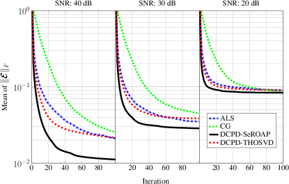
Figure 4: Mean of $\|\boldsymbol{\mathcal{E}}[R,l]\|$ per iteration for different values of SNR.

We note in this figure that DCPD-SeROAP converges more quickly than the other algorithms. For an SNR of $40$ dB, DCPD-SeROAP attains $\|\boldsymbol{\mathcal{E}}[R,l]\|\approx 0.01$ in approximately $100$ iterations while, for the other algorithms, $\|\boldsymbol{\mathcal{E}}[R,l]\|>0.02$ for the same number of iterations. Similar results are observed for other SNRs. The figure also shows that performances become similar when the SNR is decreased.

VI-E Residual vs rank

Now, we compare the algorithms for two SNRs by varying the rank of $8\times 8\times 8$ tensors.

\psfrag{T1}[cc][cc]{\footnotesize$8\times 8\times 8:$ $\text{SNR}=40\hskip 2.84526pt\text{dB}$ }\psfrag{T2}[cc][cc]{\footnotesize$8\times 8\times 8:$ $\text{SNR}=30\hskip 2.84526pt\text{dB}$ }\psfrag{A1}[cc][cc]{\footnotesize rank-$3$}\psfrag{B1}[cc][cc]{\footnotesize rank-$3$}\psfrag{A2}[cc][cc]{\footnotesize rank-$4$}\psfrag{B2}[cc][cc]{\footnotesize rank-$4$}\psfrag{A3}[cc][cc]{\footnotesize rank-$5$}\psfrag{B3}[cc][cc]{\footnotesize rank-$5$}\psfrag{A4}[cc][cc]{\footnotesize rank-$6$}\psfrag{B4}[cc][cc]{\footnotesize rank-$6$}\psfrag{A5}[cc][cc]{\footnotesize rank-$7$}\psfrag{B5}[cc][cc]{\footnotesize rank-$7$}\psfrag{Y1}[cc][cc]{\footnotesize Mean of $\|\boldsymbol{\mathcal{E}}\|$}\psfrag{Y2}[cc][cc]{\footnotesize Mean of $\|\boldsymbol{\mathcal{E}}\|$}\includegraphics[width=216.81pt]{rankvariation.eps}

Figure 5: Mean of $\|\boldsymbol{\mathcal{E}}\|$ under rank variation.

Again, we note the better performance of DCPD-SeROAP over the competing algorithms. Figure 5 also shows that the combination of DCPD and THOSVD yields the worst results. This is expected because the rank-1 approximation obtained by THOSVD is not good enough, so that DCPD does not come at a small residual.

VII Conclusion

In this paper, we presented some CP tensor decompositions algorithms and provided an analysis of their computational complexities. Our contributions included: (i) a new algebraic rank-1 method, namely SeROAP, performing better than THOSVD for three-way tensors; (ii) an iterative rank-1 approximation algorithm, namely CE, that refines any rank-1 approximation method, such as SeROAP and THOSVD, which converges in very few iterations; and (iii) an analysis of the convergence of the DCPD algorithm under a geometric point of view. Several computer experiments have confirmed the theoretical results.

Appendix A Computation of rank-1 approximation using SeROAP

We present an example of how SeROAP algorithm works for computing a rank-1 approximation of a given tensor.

Let $\boldsymbol{\mathcal{T}}$ be a $2\times 2\times 2\times 2$ complex tensor whose mode-$1$ unfolding is given by

$$\boldsymbol{T}_{(1)}=\begin{bmatrix}1&-1&0&1&3&i&0&1\\ 0&1&-i&1&1&0&2&-2i\end{bmatrix}.$$

In the first for loop of SeROAP algorithm, $\boldsymbol{v}_{1}$ is the dominate right singular vector of $\boldsymbol{V}=\boldsymbol{V}_{0}=\boldsymbol{T}_{(1)}$ given by

$$\boldsymbol{v}_{1}=\begin{bmatrix}-0.1717-0.0914i\\ 0.0245+0.1060i\\ -0.0146-0.1472i\\ -0.3189-0.0768i\\ -0.6624-0.2596i\\ -0.0914+0.1717i\\ -0.2944+0.0292i\\ -0.2010-0.3858i\end{bmatrix}.$$

By reshaping $\boldsymbol{v}_{1}$ in a $2\times 4$ matrix $\boldsymbol{V}_{1}$ we have

$$\boldsymbol{V}_{1}= \left[\begin{matrix}-0.1717-0.0914i&-0.0146-0.1472i\\ 0.0245+0.1060i&-0.3189-0.0768i\end{matrix}\right.$$

$$\qquad\left.\begin{matrix}-0.6624-0.2596i&-0.2944+0.0292i\\ -0.0914+0.1717i&-0.2010-0.3858i\end{matrix}\right].$$

In next iteration ($n=2$), we compute the dominate right singular vector of $\boldsymbol{V}=\boldsymbol{V}_{1}$. Hence,

$$\boldsymbol{v}_{2}=\begin{bmatrix}-0.1654+0.1657i\\ 0.0611+0.2758i\\ -0.6190+0.6261i\\ -0.2033+0.2210i\end{bmatrix},$$

and $\boldsymbol{V}=\boldsymbol{V}_{2}=Unvec(\boldsymbol{v}_{2})$ is updated

$$\boldsymbol{V}=\begin{bmatrix}-0.1654+0.1657i&-0.6190+0.6261i\\ 0.0611+0.2758i&-0.2033+0.2210i\end{bmatrix}.$$

The next step is to compute the vector $\boldsymbol{w}=\boldsymbol{v}^{*}\boxtimes\boldsymbol{u}$, where $\boldsymbol{u}$ and $\boldsymbol{v}$ are the first left and right singular vectors, respectively. Thus,

$$\boldsymbol{u}=\begin{bmatrix}0.6106-0.7024i\\ 0.1758-0.3208i\end{bmatrix},\boldsymbol{v}=\begin{bmatrix}-0.3027-0.0545i\\ -0.9481+0.0809i\end{bmatrix},$$

$$\boldsymbol{w}=\begin{bmatrix}-0.1466+0.2459i\\ -0.0357+0.1067i\\ -0.6357+0.6166i\\ -0.1926+0.2899i\end{bmatrix}.$$

Notice that $\boldsymbol{w}$ can be viewed as a vectorization of a rank-$1$ matrix. In the end of the first iteration of the second for loop, $\boldsymbol{w}$ is updated so that it becomes a vectorization of a rank-$1$ three-way tensor. This is achieved by performing the projection of each row of matrix $\boldsymbol{V}_{1}$ onto $\boldsymbol{w}$, by means of $\boldsymbol{V}_{1}\boldsymbol{w}$, following by the multiplication with $\boldsymbol{w}^{H}$. Hence

$$\boldsymbol{X}_{(2)}= \left[\begin{matrix}-0.1900-0.1178i&-0.0631-0.0611i\\ -0.0604+0.0051i&-0.0236-0.0031i\end{matrix}\right.$$

$$\qquad\left.\begin{matrix}-0.6624-0.1989i&-0.2377-0.1317i\\ -0.1762+0.0638i&-0.0730+0.0098i\end{matrix}\right],$$

and

$$\boldsymbol{w}=\begin{bmatrix}-0.1900-0.1178i\\ -0.0604+0.0051i\\ -0.0631-0.0611i\\ -0.0236-0.0031i\\ -0.6624-0.1989i\\ -0.1762+0.0638i\\ -0.2377-0.1317i\\ -0.0730+0.0098i\end{bmatrix}$$

In the next iteration, we perform $\boldsymbol{X}_{1}=(\boldsymbol{V}_{0})\boldsymbol{w}^{H}$, which is an unfolding of a $4$-order rank-$1$ tensor. Actually, in every iteration of the second for loop, $\boldsymbol{X}_{n}$ is updated to an unfolding of a rank-$1$ tensor of order $N-n+1$. Hence,

$$\boldsymbol{X}_{(1)}= \left[\begin{matrix}0.5373-0.0992i&0.1329+0.0653i\\ 0.2696-0.1010i&0.0750+0.0216i\end{matrix}\right.$$

$$\qquad\left.\begin{matrix}0.1981-0.0830i&0.0565+0.0140i\\ 0.0951-0.0613i&0.0306+0.0020i\end{matrix}\right.$$

$$\qquad\quad\left.\begin{matrix}1.6851+0.1360i&0.3446+0.3020i\\ 0.8868-0.0849i&0.2066+0.1249i\end{matrix}\right.$$

$$\qquad\qquad\left.\begin{matrix}0.6585-0.0886i&0.1576+0.0872i\\ 0.3335-0.1067i&0.0898+0.0307i\end{matrix}\right],$$

Indeed, $\boldsymbol{X}_{(1)}$ is the mode-$1$ unfolding of the rank-$1$ approximation of $\boldsymbol{\mathcal{T}}$ computed by SeROAP algorithm.

References

• [1] P. Comon and C. Jutten, Eds., Handbook of Blind Source Separation, Independent Component Analysis and Applications, Academic Press, Oxford UK, Burlington USA, 2010, ISBN: 978-0-12-374726-6, hal-00460653.
• [2] M. Castella and P. Comon, “Blind separation of instantaneous mixtures of dependent sources,” in Independent Component Analysis and Signal Separation, pp. 9–16. Springer, 2007.
• [3] A. L. F. de Almeida, G. Favier, and J. C. M. Mota, “Parafac-based unified tensor modeling for wireless communication systems with application to blind multiuser equalization,” Signal Processing, vol. 87, no. 2, pp. 337–351, Feb. 2007.
• [4] A. Smilde, R. Bro, and P. Geladi, Multi-way analysis: applications in the chemical sciences, John Wiley & Sons, 2005.
• [5] H. Becker, L. Albera, P. Comon, M. Haardt, G. Birot, F. Wendling, M. Gavaret, C.-G. Bénar, and I. Merlet, “Eeg extended source localization: tensor-based vs. conventional methods,” NeuroImage, vol. 96, pp. 143–157, 2014.
• [6] S. Sahnoun and P. Comon, “Joint source estimation and localization,” IEEE Trans. on Signal Processing, vol. 63, no. 10, 2015.
• [7] B. Savas, Algorithms in Data Mining using Matrix and Tensor Metho ds, Ph.D. thesis, Linköping Univ. Tech., 2008.
• [8] H. A. L. Kiers, “Towards a standardized notation and terminology in multiway analysis,” J. Chemometrics, pp. 105–122, 2000.
• [9] J. M. Ten Berge, “Kruskal’s polynomial for 2$\times$ 2$\times$ 2 arrays and a generalization to 2$\times$ n$\times$ n arrays,” Psychometrika, vol. 56, no. 4, pp. 631–636, 1991.
• [10] J. Brachat, P. Comon, B. Mourrain, and E. Tsigaridas, “Symmetric tensor decomposition,” Linear Algebra and its Applications, vol. 433, no. 11, pp. 1851–1872, 2010.
• [11] L. De Lathauwer, “A link between the canonical decomposition in multilinear algebra and simultaneous matrix diagonalization,” SIAM Journal on Matrix Analysis and Applications, vol. 28, no. 3, pp. 642–666, 2006.
• [12] L. Oeding and G. Ottaviani, “Eigenvectors of tensors and algorithms for waring decomposition,” Journal of Symbolic Computation, vol. 54, pp. 9–35, 2013.
• [13] C. J. Hillar and L.-H. Lim, “Most tensor problems are np-hard,” Journal of the ACM (JACM), vol. 60, no. 6, pp. 45, 2013.
• [14] V. De Silva and L.-H. Lim, “Tensor rank and the ill-posedness of the best low-rank approximation problem,” SIAM Journal on Matrix Analysis and Applications, vol. 30, no. 3, pp. 1084–1127, 2008.
• [15] P. Comon, X. Luciani, and A. L. F. de Almeida, “Tensor decompositions, alternating least squares and other tales,” Journal of Chemometrics, vol. 23, no. 7-8, pp. 393–405, 2009.
• [16] T. G. Kolda and B. W. Bader, “Tensor decompositions and applications,” SIAM review, vol. 51, no. 3, pp. 455–500, 2009.
• [17] M. Rajih, P. Comon, and R. A. Harshman, “Enhanced line search: A novel method to accelerate parafac,” SIAM Journal on Matrix Analysis and Applications, vol. 30, no. 3, pp. 1128–1147, 2008.
• [18] L. Sorber, M. Van Barel, and L. De Lathauwer, “Optimization-based algorithms for tensor decompositions: Canonical polyadic decomposition, decomposition in rank-(l_r,l_r,1) terms, and a new generalization,” SIAM Journal on Optimization, vol. 23, no. 2, pp. 695–720, 2013.
• [19] G. Tomasi and R. Bro, “A comparison of algorithms for fitting the parafac model,” Computational Statistics & Data Analysis, vol. 50, no. 7, pp. 1700–1734, 2006.
• [20] P. Paatero, “A weighted non-negative least squares algorithm for three-way Parafac factor analysis,” Chemometrics Intell. Lab. Syst., vol. 38, pp. 223–242, 1997.
• [21] A. Stegeman and P. Comon, “Subtracting a best rank-1 approximation does not necessarily decrease tensor rank,” Linear Algebra Appl., vol. 433, no. 7, pp. 1276–1300, Dec. 2010, hal-00512275.
• [22] A.-H. Phan, P. Tichavskỳ, and A. Cichocki, “Tensor deflation for candecomp/parafac. part 1: Alternating subspace update algorithm,” IEEE Transaction on Signal Processing, 2015.
• [23] A. Cichocki and A.-H. Phan, “Fast local algorithms for large scale nonnegative matrix and tensor factorizations,” IEICE Transactions on Fundamentals of Electronics, Communications and Computer Sciences, vol. E92-A, no. 3, pp. 708–721, 2009.
• [24] A. P. da Silva, P. Comon, and A. L. F. de Almeida, “An iterative deflation algorithm for exact cp tensor decomposition,” IEEE conference on Acoustics, Speech and Signal Processing, 2015.
• [25] L. De Lathauwer, B. De Moor, and J. Vandewalle, “A multilinear singular value decomposition,” SIAM journal on Matrix Analysis and Applications, vol. 21, no. 4, pp. 1253–1278, 2000.
• [26] L. Wang and T. chu, “On the global convergence of the alternating least squares method for rank-one approximation to generic tensors,” SIAM J. Matrix Anal. Appl., vol. 35, pp. 1058–1072, 2014.
• [27] B. Savas and L.-H. Lim, “Quasi-newton methods on grassmannians and multilinear approximations of tensors,” SIAM Journal on Scientific Computing, vol. 32, no. 6, pp. 3352–3393, 2010.
• [28] J. B. Lasserre, “Global optimization with polynomials and the problem of moments,” SIAM Journal on Optimization, vol. 11, no. 3, pp. 796–817, 2001.
• [29] M. A. Bucero and B. Mourrain, “Border basis relaxation for polynomial optimization,” arXiv preprint arXiv:1404.5489, 2014.
• [30] J. Nie and L. Wang, “Semidefinite relaxations for best rank-1 tensor approximations,” SIAM Journal on Matrix Analysis and Applications, vol. 35, no. 3, pp. 1155–1179, 2014.
• [31] G. H. Golub and C. F. Van Loan, Matrix computations, vol. 3, JHU Press, 2012.
• [32] E. Polak, Optimization: algorithms and consistent approximations, Springer-Verlag New York, Inc., 1997.
• [33] P. Comon and G. H. Golub, “Tracking a few extreme singular values and vectors in signal processing,” Proceedings of the IEEE, vol. 78, no. 8, pp. 1327–1343, 1990.
• [34] C. F. Van Loan and N. Pitsianis, Approximation with Kronecker products, Springer, 1993.