Spin-2 Form Factors at Three Loop in QCD

Abstract

Spin-2 fields are often candidates in physics beyond the Standard Model namely the models with extra-dimensions where spin-2 Kaluza-Klein gravitons couple to the fields of the SM. Also, in the context of Higgs searches, spin-2 fields have been studied as an alternative to the scalar Higgs boson. In this article, we present the complete three loop QCD radiative corrections to the spin-2 quark-antiquark and spin-2 gluon-gluon form factors in SU(N) gauge theory with $n_{f}$ light flavors. These form factors contribute to both quark-antiquark and gluon-gluon initiated processes involving spin-2 particle in the hadronic reactions at the LHC. We have studied the structure of infrared singularities in these form factors up to three loop level using Sudakov integro-differential equation and found that the anomalous dimensions originating from soft and collinear regions of the loop integrals coincide with those of the electroweak vector boson and Higgs form factors confirming the universality of the infrared singularities in QCD amplitudes.

1 Introduction

In the context of the recent discovery of the new boson at the LHC, with mass of about 125 GeV Aad:2012tfa ; Chatrchyan:2012xdj , there has been renewed interest in massive spin-2 resonance which could also lead to similar final states Ellis:2012mj . The massive spin-2 could be a Kaluza-Klein (KK) graviton of the TeV scale gravity models ADD ; Randall:1999ee as a result of gravity propagating in the extra dimensional bulk or any generic spin-2 resonance in some other new physics scenarios. It was noted in Fok:2012zk that gauge symmetry and Lorentz invariance forbid operators of dimension four that could lead to a coupling of a massive spin-2 resonance to a pair of SM particles. Further, if the flavor and CP symmetries of the SM are respected by these new physics scenarios, the leading dimension five operator is none other than the energy momentum tensor $T_{\mu\nu}$ of the SM particles. The structure of the operator coupling thus being identical to the KK graviton, though the constant coefficients could be different for the KK graviton or any generic spin-2 imposter. Nonetheless, methods to distinguish KK graviton from the imposter have been proposed Fok:2012zk and will be of importance for BSM searches at the LHC which is now operational at higher energies and luminosity. The increasing accuracy of the experimental data at the LHC Run-II, demands an equally precise theoretical predictions.

To match the current theoretical accuracy of say the Drell-Yan production Hamberg:1990np ; Ahmed:2014cla ; Catani:2014uta , the Higgs boson production in gluon fusion Harlander:2002wh ; Anastasiou:2002yz ; Ravindran:2003um ; Anastasiou:2014vaa ; Li:2014bfa ; deFlorian:2014vta ; Anastasiou:2015ema , in bottom quark annihilation Harlander:2003ai ; Ahmed:2014cha and associated production with a vector boson Brein:2003wg ; Kumar:2014uwa at the LHC, it is imperative that competing BSM models are also available to the same accuracy in higher orders in QCD. Form factors are essential ingredients for many precision calculation in QCD. An important building block for phenomenological study is the computation of $q\bar{q}\to$ spin-2 and $gg\to$ spin-2 form factors and is at present available to two-loop in QCD deFlorian:2013sza , while for many processes of interest they are now available to the 3-loop order Moch:2005tm ; Moch:2005id ; Baikov:2009bg ; Gehrmann:2010ue ; Gehrmann:2010tu ; Gehrmann:2014vha . Stringent bounds Aad:2014cka ; Chatrchyan:2012oaa ; Aad:2015mna on the parameters of ADD and RS models are available due to the presence of precise theoretical predictions for various important observables up to NLO level in QCD. Often, these observables suffer from large uncertainties resulting from renormalization and factorization scales and the only remedy to this is to include higher order QCD effects to the born contributions. The NLO QCD predictions based on fixed order as well as parton shower improved in the MadGraph5_aMC@NLO Alwall:2014hca framework for di-final state Mathews:2004xp ; Mathews:2005zs ; Kumar:2006id ; Frederix:2013lga ; Kumar:2009nn ; Frederix:2012dp ; Agarwal:2009zg ; Agarwal:2010sp ; Das:2014tva productions in the gravity mediated models have already played important role in constraining the model parameters of ADD and RS. Next-to-next-to leading order (NNLO) corrections for the graviton production at the LHC in the threshold limit are already available deFlorian:2013wpa and attempts to improve these predictions through NNLO corrections and beyond are already underway Ahmed:2014gla . As these corrections are only sensitive to the tensorial interaction and not sensitive to the details of the model, these results are applicable to production of any generic spin-2 resonance. Hence this article takes the first step towards going beyond NNLO for the resonant production of a generic spin-2 particle at the LHC, namely the computation of quark and gluon form factors at three loop level in perturbative QCD with $n_{f}$ light flavors. We will report the first results on the threshold effects at N³LO in the future publication and demonstrate the importance such corrections at the LHC in the context of spin-2 resonance searches.

In addition to the phenomenological importance with respect to precise predictions of some observable, form factors in QCD are of considerable theoretical interest in terms of the factorization and universal nature of the singular structure. Studying the infrared pole structure and factorization properties of these IR singularities in multi-loop QCD amplitudes with tensorial coupling to 3-loop order and to confirm the standard expectation of QCD amplitudes Catani:1998bh ; Sterman:2002qn ; Becher:2009cu ; Gardi:2009qi is an essential prerequisite. The spin-2 field being a tensor of rank-2 is coupled to the energy-momentum tensor $T_{\mu\nu}$, which is a symmetric and conserved quantity. The operator $T_{\mu\nu}$ of QCD is finite Nielsen:1977sy , which would imply no UV renormalization is required. Further $T_{\mu\nu}$ consists of gauge invariant terms and in addition gauge dependent and ghost terms, we explicitly observe that to the 3-loop order these form factors are independent of the gauge dependent and ghost terms Nielsen:1977sy ; Zoller:2012qv , which is an important check of the calculation. From a computational point of view 3-loop amplitudes with higher tensorial coupling is being attempted for the first time. At the intermediate stages of the computation this leads to higher rank tensorial integrals resulting from more than 3000 three loop Feynman amplitudes contributing to the gluon form factor alone. This computation again establishes the power of several state-of-the-art techniques namely IBP and LI identities and differential equation method to solve the master integrals.

In the next section 2, we describe the effective Lagrangian. In section 3, after defining the quark and gluon form factors, we present the computational details at three loop level followed by the results. The details of ultraviolet renormalization and universal structure of infrared poles are given in section 4 and section 5 respectively. Finally we conclude with our findings in section 6.

2 The Effective Lagrangian

The effective Lagrangian that describes the interaction of the spin-2 field with the SM fields can be written down in a gauge invariant way through the energy momentum tensor of the SM fields. We denote the spin-2 field by $h^{\mu\nu}$ and the SM energy momentum tensor by $T_{\mu\nu}^{SM}$. Since we are interested only in the QCD corrections to processes involving spin-2 fields, we restrict ourselves to the QCD part of $T_{\mu\nu}^{SM}$ and the corresponding action reads ADD ; Randall:1999ee as

$${\cal S}={\cal S}_{SM}+{\cal S}_{h}-\frac{\kappa}{2}\int d^{4}x~{}T^{QCD}_{\mu\nu}(x)~{}h^{\mu\nu}(x)\,,$$ (1)

where ${\cal S}_{SM}$ is the SM action, ${\cal S}_{h}$ is the kinetic energy part of the action corresponding to spin-2 fields, $\kappa$ is a dimensionful coupling and $T^{QCD}_{\mu\nu}$ is the energy momentum tensor of QCD given by

$$T^{QCD}_{\mu\nu} = -g_{\mu\nu}{\cal L}_{QCD}-F_{\mu\rho}^{a}F^{a\rho}_{\nu}-\frac{1}{\xi}g_{\mu\nu}\partial^{\rho}(A_{\rho}^{a}\partial^{\sigma}A_{\sigma}^{a})+\frac{1}{\xi}(A_{\nu}^{a}\partial_{\mu}(\partial^{\sigma}A_{\sigma}^{a})+A_{\mu}^{a}\partial_{\nu}(\partial^{\sigma}A_{\sigma}^{a}))$$ (2)

$$+\frac{i}{4}\Big{[}\overline{\psi}\gamma_{\mu}(\overrightarrow{\partial}_{\nu}-ig_{s}T^{a}A^{a}_{\nu})\psi-\overline{\psi}(\overleftarrow{\partial}_{\nu}+ig_{s}T^{a}A^{a}_{\nu})\gamma_{\mu}\psi+\overline{\psi}\gamma_{\nu}(\overrightarrow{\partial}_{\mu}-ig_{s}T^{a}A^{a}_{\mu})\psi$$

$$-\overline{\psi}(\overleftarrow{\partial}_{\mu}+ig_{s}T^{a}A^{a}_{\mu})\gamma_{\nu}\psi\Big{]}+\partial_{\mu}\overline{\omega}^{a}(\partial_{\nu}\omega^{a}-g_{s}f^{abc}A_{\nu}^{c}\omega^{b})$$

$$+\partial_{\nu}\overline{\omega}^{a}(\partial_{\mu}\omega^{a}-g_{s}f^{abc}A_{\mu}^{c}\omega^{b}).$$

$g_{s}$ is the strong coupling constant and $\xi$ is the gauge fixing parameter. The $T^{a}$ are generators and $f^{abc}$ are the structure constants of $SU(3)$. Note that spin-2 fields couple to ghost fields ($\omega^{a}$) Mathews:2004pi as well in order to cancel unphysical degrees of freedom of gluon fields ($A^{a}_{\mu}$).

3 The Form Factors

The form factor parametrizes the interaction of the spin-2 field with those of SM order by order in perturbation theory. We compute both quark and gluon form factors by sandwiching the energy-momentum tensor between on-shell quark and gluon states respectively normalized by their respective born amplitudes:

$$\hat{\cal F}^{T}_{\rm I}(Q^{2},\epsilon) = \frac{\hat{\cal M}_{\rm I}^{(0)*}.M_{\rm I}}{\hat{\cal M}_{\rm I}^{(0)*}.\hat{\cal M}_{\rm I}^{(0)}}$$ (3)

$$= \sum_{n=0}^{\infty}\hat{a}_{s}^{n}\left(\frac{Q^{2}}{\mu^{2}}\right)^{n{\epsilon\over 2}}S_{\epsilon}^{n}\hat{\cal F}^{T,(n)}_{\rm I}(\epsilon),\quad\quad\quad I=q,g$$

where $M_{\rm I}$ are the unrenormalized amplitudes computed in powers of the bare strong coupling constant $\hat{a}_{s}=\hat{g}_{s}^{2}/16\pi^{2}$ using dimensional regularization in $d=4+\epsilon$ dimensions, that is

$$M_{\rm I}(Q^{2},\epsilon)=\sum_{n=0}^{\infty}\hat{a}_{s}^{n}\left(\frac{Q^{2}}{\mu^{2}}\right)^{n{\epsilon\over 2}}S_{\epsilon}^{n}\hat{\cal M}^{(n)}_{\rm I}(\epsilon),$$ (4)

where $Q^{2}=-2p_{1}\cdot p_{2}$ and $p_{1}$, $p_{2}$ are the momenta of external quark or gluon on-shell states. The dimensionful scale $\mu$ is introduced to keep the strong coupling constant dimensionless in $d$ space-time dimensions. The other constant at $n^{\rm th}$ loop is $S_{\epsilon}^{n}=\exp[\frac{n\epsilon}{2}(\gamma_{E}-\ln 4\pi)]$ where Euler constant $\gamma_{E}=0.5772\ldots$.

In deFlorian:2013sza , both one and two loop form factors were presented in dimensional regularization and later on, they were used in deFlorian:2013wpa to compute the threshold corrections to Drell-Yan production at the LHC in ADD and RS models to second order in strong coupling constant. In the following, we present the third order correction to the form factors in QCD.

3.1 Computational Procedure

In this section, we describe in detail the method that we follow to compute both quark and gluon form factors of the energy momentum tensor to third order in strong coupling constant using dimensional regularization. The relevant amplitudes are generated using QGRAF Nogueira:1991ex . At third order alone, there are 3374 and 1072 number of Feynman diagrams for gluon and quark form factors respectively. The QGRAF generated amplitudes are then converted into a suitable format using routines developed using the symbolic manipulation program FORM Vermaseren:2000nd . Both group as well as Lorentz indices are carefully handled to express the form factors in a suitable color basis involving Casimir operators of $SU(N)$ with the coefficients containing three loop scalar integrals. For the gluon form factor we have summed only the physical polarizations of the external gluons using

$$\sum_{s}\varepsilon^{\mu}(p_{i},s)\varepsilon^{\nu*}(p_{i},s)=-g^{\mu\nu}+\frac{p_{i}^{\mu}q_{i}^{\nu}+q_{i}^{\mu}p_{i}^{\nu}}{p_{i}.q_{i}}$$ (5)

where, $p_{i}$ is the $i^{th}$-gluon momentum and $q_{i}$ is the corresponding light-like momentum. We choose $q_{1}=p_{2}$ and $q_{2}=p_{1}$ for simplicity. For the external spin-2 fields, we have used the $d$ dimensional polarization sum given in Mathews:2004xp with $q$ being the spin-2 momentum

$$B^{\mu\nu;\rho\sigma}(q) = \left(g^{\mu\rho}-\frac{\,\,q^{\mu}q^{\rho}}{q.q}\right)\left(g^{\nu\sigma}-\frac{\,\,q^{\nu}q^{\sigma}}{q.q}\right)+\left(g^{\mu\sigma}-\frac{\,\,q^{\mu}q^{\sigma}}{q.q}\right)\left(g^{\nu\rho}-\frac{\,\,q^{\nu}q^{\rho}}{q.q}\right)$$ (6)

$$-\,\,\frac{2}{d-1}\left(g^{\mu\nu}-\frac{\,\,q^{\mu}q^{\nu}}{q.q}\right)\left(g^{\rho\sigma}-\frac{\,\,q^{\rho}q^{\sigma}}{q.q}\right)\,.$$

We have used Feynman gauge throughout.

At three loop level, we find that the diagrams contributing to form factors can have at most 9 independent propagators involving two external momenta $p_{1},p_{2}$ and three internal loop momenta $k_{1},k_{2},k_{3}$, while the maximum number of scalar products that can appear in the numerator of each diagram can be 12. Hence we need to increase the number of propagators to 12 which allow us to classify all the three loop diagrams into three different auxiliary topologies. We take the help of Reduze2 vonManteuffel:2012np for this purpose. The topologies Gehrmann:2010ue that are used in our computation are given below

$${\rm A}_{1} :~{}~{}{\cal D}_{1},{\cal D}_{2},{\cal D}_{3},{\cal D}_{12},{\cal D}_{13},{\cal D}_{23},{\cal D}_{1;1},{\cal D}_{1:12},{\cal D}_{2;1},{\cal D}_{2:12},{\cal D}_{3;1},{\cal D}_{3:12}$$

$${\rm A}_{2} :~{}~{}{\cal D}_{1},{\cal D}_{2},{\cal D}_{3},{\cal D}_{12},{\cal D}_{13},{\cal D}_{23},{\cal D}_{13;2},{\cal D}_{1:12},{\cal D}_{2;1},{\cal D}_{12:2},{\cal D}_{3;1},{\cal D}_{3:12}$$

$${\rm A}_{3} :~{}~{}{\cal D}_{1},{\cal D}_{2},{\cal D}_{3},{\cal D}_{12},{\cal D}_{13},{\cal D}_{123},{\cal D}_{1;1},{\cal D}_{1:12},{\cal D}_{2;1},{\cal D}_{2:12},{\cal D}_{3;1},{\cal D}_{3:12}$$ (7)

where,

$${\cal D}_{i}=k_{i}^{2},~{}{\cal D}_{ij}=(k_{i}-k_{j})^{2},~{}{\cal D}_{ijl}=(k_{i}-k_{j}-k_{l})^{2},\hskip 28.45274pt$$

$${\cal D}_{i;j}=(k_{i}-p_{j})^{2},~{}{\cal D}_{i;jl}=(k_{i}-p_{j}-p_{l})^{2},~{}{\cal D}_{ij;l}=(k_{i}-k_{j}-p_{l})^{2}\,.$$ (8)

The resulting integrals classified in terms of three topologies, are then reduced to a set of master integrals by using a systematic approach that uses Integration by parts (IBP) chet and Lorentz invariant (LI) gr identities. The IBP identities follow from the fact that within dimensional regularization, the integrals are finite and well-behaved and hence any integrand at the boundary must be zero. Following this, the generalization of Gauss theorem implies the integral of the total derivative with respect to any loop momenta to be zero, that is

$$\int\frac{d^{d}k_{1}}{(2\pi)^{d}}\cdot\cdot\cdot\int\frac{d^{d}k_{3}}{(2\pi)^{d}}\frac{\partial}{\partial k_{i}}\cdot\left(v_{j}\frac{1}{\prod_{l}D_{l}^{n_{l}}}\right)=0\,,$$ (9)

where $n_{l}$ is an element of $\vec{n}=(n_{1},\cdot\cdot\cdot,n_{12})$ with $n_{l}\in Z$ and $D_{l}$s are propagators which depend on the loop and external momenta. The four vector $v_{j}^{\mu}$ can be both loop and external momenta. Performing the differentiation on the left hand side and expressing the scalar products of $k_{i}$ and $p_{j}$ linearly in terms of ${\cal D}_{l}$’s, one obtains the IBP identities given by

$$\sum_{i}a_{i}J(b_{i,1}+n_{1},...,b_{i,12}+n_{12})=0$$ (10)

where

$$J(\vec{m})=J(m_{1},\cdot\cdot\cdot,m_{12})=\int\frac{d^{d}k_{1}}{(2\pi)^{d}}\cdot\cdot\cdot\frac{d^{d}k_{3}}{(2\pi)^{d}}\frac{1}{\prod_{l}D_{l}^{m_{l}}}$$ (11)

with $b_{i,j}\in\{-1,0,1\}$ and $a_{i}$ are polynomial in $n_{j}$. The LI identities follow from the fact that the loop integrals are invariant under Lorentz transformations of the external momenta, that is

$$p_{i}^{\mu}p_{j}^{\nu}\left(\sum_{k}p_{k[\nu}\frac{\partial}{\partial p_{k}^{\mu]}}\right)J(\vec{n})=0.$$ (12)

For the case of three loop form factor, there are 15 IBP identities and 1 LI identity for each integrand, and hence there are large number of equations for the whole system. These equations can be solved to relate the large number of scalar integrals and express them in terms of a set of fewer integrals which are the so called master integrals. To solve this large system of equations, there are dedicated computer algebra tools like AIR Anastasiou:2004vj , FIRE Smirnov:2008iw , REDUZE Studerus:2009ye ; vonManteuffel:2012np , LiteRed Lee:2012cn ; Lee:2013mka etc. We use the Mathematica based package LiteRedV1.82 along with MintV1.1 Lee:2013hzt .

We find that the form factors at three loop level can be expressed in terms of 22 master integrals. Following the same notation as of Gehrmann:2010ue , the master integrals can be distinguished into three topological types: genuine three loop integrals with vertex functions ($A_{t,i}$), three loop propagator integrals ($B_{t,i}$) and integrals which are product of one loop and two loop integrals ($C_{t,i}$). Defining a generic three loop master integral as

$$A_{i,m_{1}^{i}m_{2}^{i}\cdots m_{12}^{i}}=\int\frac{d^{d}k_{1}}{(2\pi)^{d}}\int\frac{d^{d}k_{2}}{(2\pi)^{d}}\int\frac{d^{d}k_{3}}{(2\pi)^{d}}\frac{1}{\prod_{j}D_{j}^{m_{j}^{i}}},\quad\quad\quad i=1,2,3$$ (13)

where $D_{j}$ is the $j^{\rm th}$ element of the set $A_{i}$, we can identify the resulting master integrals in our computation with those given in Gehrmann:2010ue and they are listed in Fig. 1 and Fig. 2.

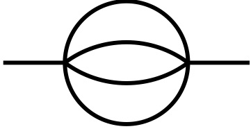
$B_{4,1}\equiv A_{1,001101010000}$

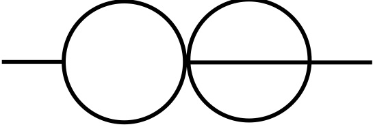
$B_{5,1}\equiv A_{1,011010010100}$

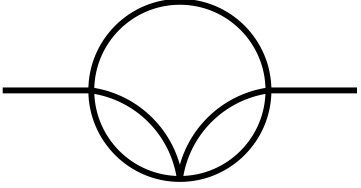
$B_{5,2}\equiv A_{1,001011010100}$

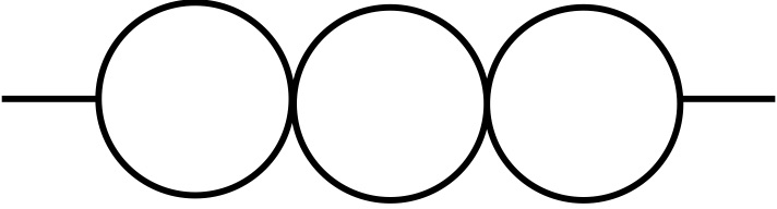
$B_{6,1}\equiv A_{1,111000010101}$

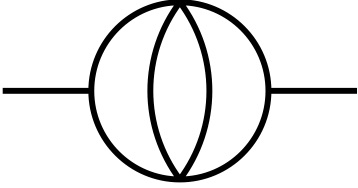
$B_{6,2}\equiv A_{1,011110000101}$

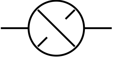
$B_{8,1}\equiv A_{3,011111010101}$

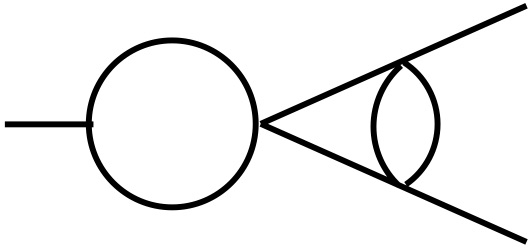
$C_{6,1}\equiv A_{1,011100100101}$

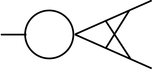
$C_{8,1}\equiv A_{2,111100011101}$

Figure 1: Two point and factorizable three point three loop integrals

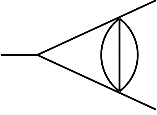
$A_{5,1}\equiv A_{1,001101100001}$

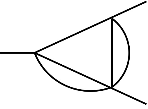
$A_{5,2}\equiv A_{1,001011011000}$

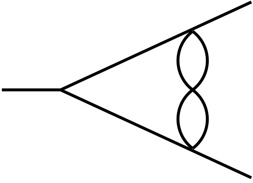
$A_{6,1}\equiv A_{1,010101100110}$

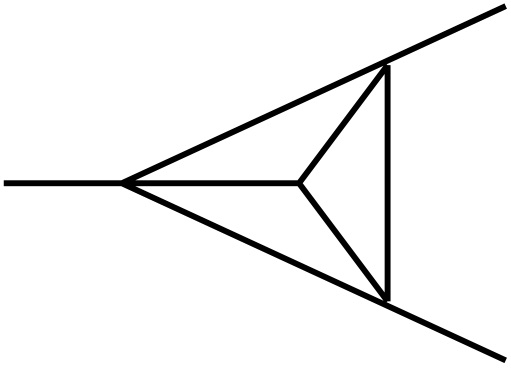
$A_{6,2}\equiv A_{1,001111011000}$

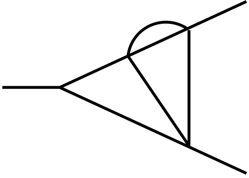
$A_{6,3}\equiv A_{1,001110100101}$

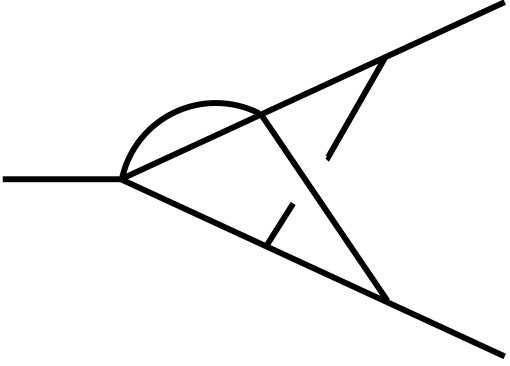
$A_{7,1}\equiv A_{2,011110011100}$

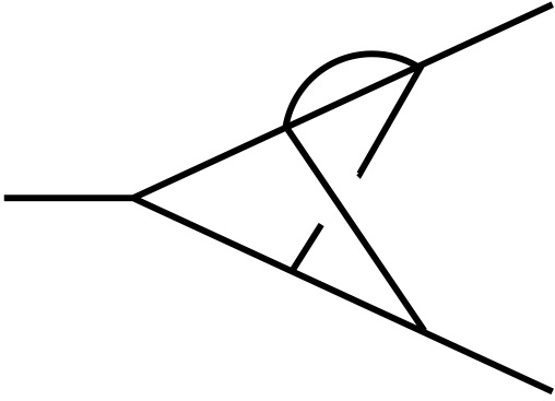
$A_{7,2}\equiv A_{2,011011001101}$

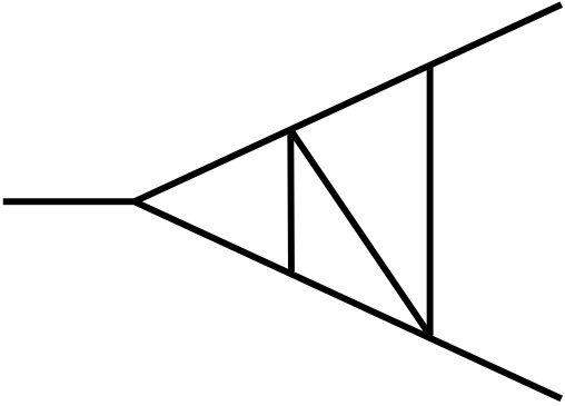
$A_{7,3}\equiv A_{1,011011110100}$

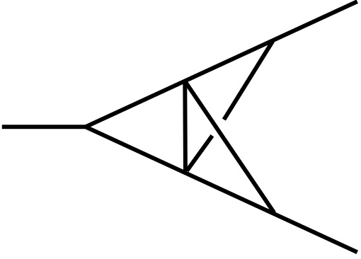
$A_{7,4}\equiv A_{2,011110001101}$

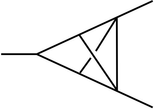
$A_{7,5}\equiv A_{2,011011010101}$

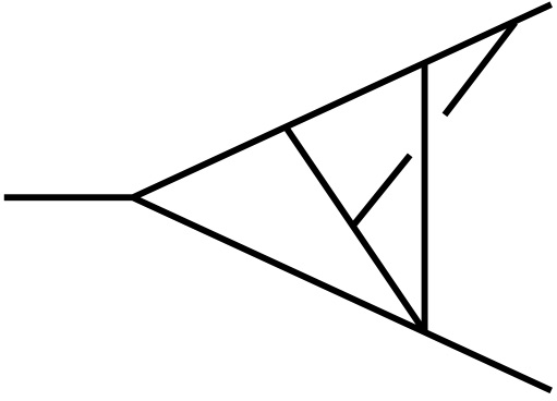
$A_{8,1}\equiv A_{2,001111011101}$

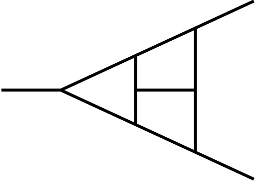
$A_{9,1}\equiv A_{1,011111110110}$

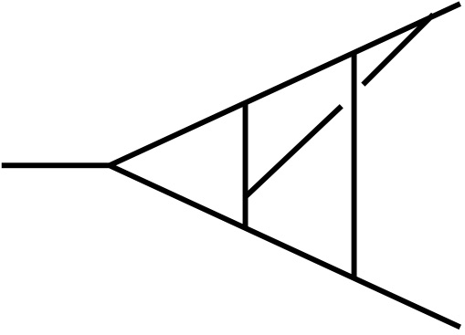
$A_{9,2}\equiv A_{2,011111011101}$

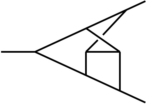
$A_{9,4}\equiv A_{2,111011111100}$

Figure 2: Genuine three loop integrals with vertex function

The master integrals were computed in Baikov:2009bg ; Gehrmann:2010ue to relevant orders in $\epsilon$ and we have used them to complete our computation of the form factors up to three loop level. The electronic version of the results of both quark and gluon form factors in terms of the master integrals $A_{i,j},B_{i,j}$ and $C_{i,j}$ for arbitrary $d$ is attached with the arXiv version. In the next section, we present the three loop results for both the form factors expanded in powers of $\epsilon$ along with already known one and two loop results.

3.2 Results

In this section we present one, two and three loop quark and gluon form factors after expanding in powers of $\epsilon$ to relevant order. The one and two loop results completely agree with deFlorian:2013sza and the three loop ones are new.

$$\hat{\cal F}^{T,(1)}_{g} =C_{A}\Bigg{\{}-\frac{8}{\epsilon^{2}}+\frac{1}{\epsilon}\frac{22}{3}-\frac{203}{18}+\zeta_{2}+\epsilon\Bigg{(}\frac{2879}{216}-\frac{7}{3}\zeta_{3}-\frac{11}{12}\zeta_{2}\Bigg{)}+\epsilon^{2}\Bigg{(}-\frac{37307}{2592}+\frac{77}{36}\zeta_{3}$$

$$+\frac{203}{144}\zeta_{2}+\frac{47}{80}\zeta_{2}^{2}\Bigg{)}+\epsilon^{3}\Bigg{(}\frac{465143}{31104}-\frac{31}{20}\zeta_{5}-\frac{1421}{432}\zeta_{3}-\frac{2879}{1728}\zeta_{2}+\frac{7}{24}\zeta_{2}\zeta_{3}-\frac{517}{960}\zeta_{2}^{2}\Bigg{)}$$

$$+\epsilon^{4}\Bigg{(}-\frac{5695811}{373248}+\frac{341}{240}\zeta_{5}+\frac{20153}{5184}\zeta_{3}-\frac{49}{144}\zeta_{3}^{2}+\frac{37307}{20736}\zeta_{2}-\frac{77}{288}\zeta_{2}\zeta_{3}+\frac{9541}{11520}\zeta_{2}^{2}$$

$$+\frac{949}{4480}\zeta_{2}^{3}\Bigg{)}\Bigg{\}}+n_{f}\Bigg{\{}-\frac{4}{3}\frac{1}{\epsilon}+\frac{35}{18}+\epsilon\Bigg{(}-\frac{497}{216}+\frac{1}{6}\zeta_{2}\Bigg{)}+\epsilon^{2}\Bigg{(}\frac{6593}{2592}-\frac{7}{18}\zeta_{3}-\frac{35}{144}\zeta_{2}\Bigg{)}$$

$$+\epsilon^{3}\Bigg{(}-\frac{84797}{31104}+\frac{245}{432}\zeta_{3}+\frac{497}{1728}\zeta_{2}+\frac{47}{480}\zeta_{2}^{2}\Bigg{)}+\epsilon^{4}\Bigg{(}\frac{1072433}{373248}-\frac{31}{120}\zeta_{5}-\frac{3479}{5184}\zeta_{3}$$

$$-\frac{6593}{20736}\zeta_{2}+\frac{7}{144}\zeta_{2}\zeta_{3}-\frac{329}{2304}\zeta_{2}^{2}\Bigg{)}\Bigg{\}}\,,$$

$$\hat{\cal F}^{T,(1)}_{q} =C_{F}\Bigg{\{}-\frac{8}{\epsilon^{2}}+\frac{6}{\epsilon}-10+\zeta_{2}+\epsilon\Bigg{(}12-\frac{7}{3}\zeta_{3}-\frac{3}{4}\zeta_{2}\Bigg{)}+\epsilon^{2}\Bigg{(}-13+\frac{7}{4}\zeta_{3}+\frac{5}{4}\zeta_{2}+\frac{47}{80}\zeta_{2}^{2}\Bigg{)}$$

$$+\epsilon^{3}\Bigg{(}\frac{27}{2}-\frac{31}{20}\zeta_{5}-\frac{35}{12}\zeta_{3}-\frac{3}{2}\zeta_{2}+\frac{7}{24}\zeta_{2}\zeta_{3}-\frac{141}{320}\zeta_{2}^{2}\Bigg{)}+\epsilon^{4}\Bigg{(}-\frac{55}{4}+\frac{93}{80}\zeta_{5}+\frac{7}{2}\zeta_{3}$$

$$-\frac{49}{144}\zeta_{3}^{2}+\frac{13}{8}\zeta_{2}-\frac{7}{32}\zeta_{2}\zeta_{3}+\frac{47}{64}\zeta_{2}^{2}+\frac{949}{4480}\zeta_{2}^{3}\Bigg{)}\Bigg{\}}\,,$$ (14)

$$\hat{\cal F}^{T,(2)}_{g} =C_{A}^{2}\Bigg{\{}\frac{32}{\epsilon^{4}}-\frac{44}{\epsilon^{3}}+\frac{1}{\epsilon^{2}}\Bigg{(}\frac{226}{3}-4\zeta_{2}\Bigg{)}+\frac{1}{\epsilon}\Bigg{(}-81+\frac{50}{3}\zeta_{3}+\frac{11}{3}\zeta_{2}\Bigg{)}+\frac{5249}{108}-11\zeta_{3}$$

$$-\frac{67}{18}\zeta_{2}-\frac{21}{5}\zeta_{2}^{2}+\epsilon\Bigg{(}\frac{59009}{1296}-\frac{71}{10}\zeta_{5}+\frac{433}{18}\zeta_{3}-\frac{337}{108}\zeta_{2}-\frac{23}{6}\zeta_{2}\zeta_{3}+\frac{99}{40}\zeta_{2}^{2}\Bigg{)}$$

$$+\epsilon^{2}\Bigg{(}-\frac{1233397}{5184}+\frac{759}{20}\zeta_{5}-\frac{8855}{216}\zeta_{3}+\frac{901}{36}\zeta_{3}^{2}+\frac{12551}{648}\zeta_{2}+\frac{77}{36}\zeta_{2}\zeta_{3}-\frac{4843}{720}\zeta_{2}^{2}$$

$$+\frac{2313}{280}\zeta_{2}^{3}\Bigg{)}\Bigg{\}}+C_{A}n_{f}\Bigg{\{}\frac{8}{\epsilon^{3}}+\frac{1}{\epsilon^{2}}\Bigg{(}-\frac{40}{3}\Bigg{)}+\frac{1}{\epsilon}\Bigg{(}\frac{41}{3}-\frac{2}{3}\zeta_{2}\Bigg{)}-\frac{605}{108}+10\zeta_{3}+\frac{5}{9}\zeta_{2}$$

$$+\epsilon\Bigg{(}-\frac{21557}{1296}-\frac{182}{9}\zeta_{3}+\frac{145}{108}\zeta_{2}-\frac{57}{20}\zeta_{2}^{2}\Bigg{)}+\epsilon^{2}\Bigg{(}\frac{320813}{5184}+\frac{71}{10}\zeta_{5}+\frac{6407}{216}\zeta_{3}-\frac{3617}{648}\zeta_{2}$$

$$-\frac{43}{18}\zeta_{2}\zeta_{3}+\frac{1099}{180}\zeta_{2}^{2}\Bigg{)}\Bigg{\}}+C_{F}n_{f}\Bigg{\{}-\frac{2}{\epsilon}+\frac{61}{6}-8\zeta_{3}+\epsilon\Bigg{(}-\frac{2245}{72}+\frac{59}{3}\zeta_{3}+\frac{1}{2}\zeta_{2}$$

$$+\frac{12}{5}\zeta_{2}^{2}\Bigg{)}+\epsilon^{2}\Bigg{(}\frac{64177}{864}-14\zeta_{5}-\frac{335}{9}\zeta_{3}-\frac{83}{24}\zeta_{2}+2\zeta_{2}\zeta_{3}-\frac{179}{30}\zeta_{2}^{2}\Bigg{)}\Bigg{\}}\,,$$ (15)

$$\hat{\cal F}^{T,(2)}_{q} =C_{F}^{2}\Bigg{\{}\frac{32}{\epsilon^{4}}-\frac{48}{\epsilon^{3}}+\frac{1}{\epsilon^{2}}\Bigg{(}98-8\zeta_{2}\Bigg{)}+\frac{1}{\epsilon}\Bigg{(}-\frac{309}{2}+\frac{128}{3}\zeta_{3}\Bigg{)}+\frac{5317}{24}-90\zeta_{3}+\frac{41}{2}\zeta_{2}$$

$$-13\zeta_{2}^{2}+\epsilon\Bigg{(}-\frac{28127}{96}+\frac{92}{5}\zeta_{5}+\frac{1327}{6}\zeta_{3}-\frac{1495}{24}\zeta_{2}-\frac{56}{3}\zeta_{2}\zeta_{3}+\frac{173}{6}\zeta_{2}^{2}\Bigg{)}$$

$$+\epsilon^{2}\Bigg{(}\frac{1244293}{3456}-\frac{311}{10}\zeta_{5}-\frac{34735}{72}\zeta_{3}+\frac{652}{9}\zeta_{3}^{2}+\frac{38543}{288}\zeta_{2}+\frac{193}{6}\zeta_{2}\zeta_{3}-\frac{10085}{144}\zeta_{2}^{2}$$

$$+\frac{223}{20}\zeta_{2}^{3}\Bigg{)}\Bigg{\}}+C_{A}C_{F}\Bigg{\{}\frac{44}{3}\frac{1}{\epsilon^{3}}+\frac{1}{\epsilon^{2}}\Bigg{(}-\frac{332}{9}+4\zeta_{2}\Bigg{)}+\frac{1}{\epsilon}\Bigg{(}\frac{4921}{54}-26\zeta_{3}+\frac{11}{3}\zeta_{2}\Bigg{)}$$

$$-\frac{120205}{648}+\frac{755}{9}\zeta_{3}-\frac{251}{9}\zeta_{2}+\frac{44}{5}\zeta_{2}^{2}+\epsilon\Bigg{(}\frac{2562925}{7776}-\frac{51}{2}\zeta_{5}-\frac{5273}{27}\zeta_{3}+\frac{14761}{216}\zeta_{2}$$

$$+\frac{89}{6}\zeta_{2}\zeta_{3}-\frac{3299}{120}\zeta_{2}^{2}\Bigg{)}+\epsilon^{2}\Bigg{(}-\frac{50471413}{93312}+\frac{3971}{60}\zeta_{5}+\frac{282817}{648}\zeta_{3}-\frac{569}{12}\zeta_{3}^{2}-\frac{351733}{2592}\zeta_{2}$$

$$-\frac{1069}{36}\zeta_{2}\zeta_{3}+\frac{7481}{120}\zeta_{2}^{2}-\frac{809}{280}\zeta_{2}^{3}\Bigg{)}\Bigg{\}}+C_{F}n_{f}\Bigg{\{}-\frac{8}{3}\frac{1}{\epsilon^{3}}+\frac{56}{9}\frac{1}{\epsilon^{2}}+\frac{1}{\epsilon}\Bigg{(}-\frac{425}{27}-\frac{2}{3}\zeta_{2}\Bigg{)}$$

$$+\frac{9989}{324}-\frac{26}{9}\zeta_{3}+\frac{38}{9}\zeta_{2}+\epsilon\Bigg{(}-\frac{202253}{3888}+\frac{2}{27}\zeta_{3}-\frac{989}{108}\zeta_{2}+\frac{41}{60}\zeta_{2}^{2}\Bigg{)}$$

$$+\epsilon^{2}\Bigg{(}\frac{3788165}{46656}-\frac{121}{30}\zeta_{5}-\frac{935}{324}\zeta_{3}+\frac{22937}{1296}\zeta_{2}-\frac{13}{18}\zeta_{2}\zeta_{3}+\frac{97}{180}\zeta_{2}^{2}\Bigg{)}\Bigg{\}}\,,$$ (16)

$$\hat{\cal F}^{T,(3)}_{g} =C_{A}^{3}\Bigg{\{}\frac{1}{\epsilon^{6}}\Bigg{(}-\frac{256}{3}\Bigg{)}+\frac{1}{\epsilon^{5}}\Bigg{(}\frac{352}{3}\Bigg{)}+\frac{1}{\epsilon^{4}}\Bigg{(}-\frac{14744}{81}\Bigg{)}+\frac{1}{\epsilon^{3}}\Bigg{(}\frac{13126}{243}-\frac{176}{3}\zeta_{3}+\frac{484}{27}\zeta_{2}\Bigg{)}$$

$$+\frac{1}{\epsilon^{2}}\Bigg{(}\frac{149939}{486}-\frac{440}{27}\zeta_{3}-\frac{4321}{81}\zeta_{2}+\frac{494}{45}\zeta_{2}^{2}\Bigg{)}+\frac{1}{\epsilon}\Bigg{(}-\frac{14639165}{17496}+\frac{1756}{15}\zeta_{5}-\frac{634}{9}\zeta_{3}$$

$$+\frac{112633}{972}\zeta_{2}+\frac{170}{9}\zeta_{2}\zeta_{3}+\frac{4213}{180}\zeta_{2}^{2}\Bigg{)}+\frac{1056263429}{1049760}+\frac{5014}{45}\zeta_{5}+\frac{539}{2430}\zeta_{3}-\frac{1766}{9}\zeta_{3}^{2}$$

$$-\frac{1988293}{11664}\zeta_{2}-\frac{92}{9}\zeta_{2}\zeta_{3}-\frac{64997}{2160}\zeta_{2}^{2}-\frac{22523}{270}\zeta_{2}^{3}\Bigg{\}}+C_{A}^{2}n_{f}\Bigg{\{}\frac{1}{\epsilon^{5}}\Bigg{(}-\frac{64}{3}\Bigg{)}+\frac{1}{\epsilon^{4}}\Bigg{(}\frac{1840}{81}\Bigg{)}$$

$$+\frac{1}{\epsilon^{3}}\Bigg{(}\frac{5818}{243}-\frac{88}{27}\zeta_{2}\Bigg{)}+\frac{1}{\epsilon^{2}}\Bigg{(}-\frac{56783}{486}-\frac{1456}{27}\zeta_{3}+\frac{892}{81}\zeta_{2}\Bigg{)}+\frac{1}{\epsilon}\Bigg{(}\frac{3370273}{17496}+\frac{5831}{81}\zeta_{3}$$

$$-\frac{26173}{972}\zeta_{2}+\frac{1153}{90}\zeta_{2}^{2}\Bigg{)}+\frac{5797271}{1049760}-\frac{11528}{45}\zeta_{5}+\frac{5401}{30}\zeta_{3}+\frac{489781}{11664}\zeta_{2}+\frac{2}{9}\zeta_{2}\zeta_{3}$$

$$-\frac{923}{72}\zeta_{2}^{2}\Bigg{\}}+C_{A}n_{f}^{2}\Bigg{\{}\frac{1}{\epsilon^{4}}\Bigg{(}\frac{160}{81}\Bigg{)}+\frac{1}{\epsilon^{3}}\Bigg{(}-\frac{1340}{243}\Bigg{)}+\frac{1}{\epsilon^{2}}\Bigg{(}7-\frac{4}{27}\zeta_{2}\Bigg{)}+\frac{1}{\epsilon}\Bigg{(}\frac{45077}{8748}$$

$$+\frac{940}{81}\zeta_{3}-\frac{5}{162}\zeta_{2}\Bigg{)}-\frac{32220173}{524880}-\frac{122141}{2430}\zeta_{3}+\frac{661}{216}\zeta_{2}-\frac{1777}{540}\zeta_{2}^{2}\Bigg{\}}$$

$$+C_{A}C_{F}n_{f}\Bigg{\{}\frac{1}{\epsilon^{3}}\Bigg{(}\frac{128}{9}\Bigg{)}+\frac{1}{\epsilon^{2}}\Bigg{(}-\frac{1712}{27}+\frac{512}{9}\zeta_{3}\Bigg{)}+\frac{1}{\epsilon}\Bigg{(}\frac{11732}{81}-\frac{2360}{27}\zeta_{3}-\frac{8}{3}\zeta_{2}$$

$$-\frac{256}{15}\zeta_{2}^{2}\Bigg{)}-\frac{152656}{1215}+\frac{1256}{9}\zeta_{5}-\frac{10754}{405}\zeta_{3}+\frac{34}{3}\zeta_{2}+\frac{132}{5}\zeta_{2}^{2}\Bigg{\}}+C_{F}^{2}n_{f}\Bigg{\{}\frac{1}{\epsilon}\Bigg{(}\frac{2}{3}\Bigg{)}$$

$$-\frac{241}{18}+80\zeta_{5}-\frac{148}{3}\zeta_{3}\Bigg{\}}+C_{F}n_{f}^{2}\Bigg{\{}\frac{1}{\epsilon^{2}}\Bigg{(}-\frac{16}{9}\Bigg{)}+\frac{1}{\epsilon}\Bigg{(}\frac{388}{27}-\frac{32}{3}\zeta_{3}\Bigg{)}-\frac{5623}{81}$$

$$+\frac{412}{9}\zeta_{3}+\frac{2}{3}\zeta_{2}+\frac{16}{5}\zeta_{2}^{2}\Bigg{\}}\,,$$ (17)

$$\hat{\cal F}^{T,(3)}_{q} =C_{F}^{3}\Bigg{\{}\frac{1}{\epsilon^{6}}\Bigg{(}-\frac{256}{3}\Bigg{)}+\frac{1}{\epsilon^{5}}\Bigg{(}192\Bigg{)}+\frac{1}{\epsilon^{4}}\Bigg{(}-464+32\zeta_{2}\Bigg{)}+\frac{1}{\epsilon^{3}}\Bigg{(}888-\frac{800}{3}\zeta_{3}+24\zeta_{2}\Bigg{)}$$

$$+\frac{1}{\epsilon^{2}}\Bigg{(}-\frac{4582}{3}+808\zeta_{3}-258\zeta_{2}+\frac{426}{5}\zeta_{2}^{2}\Bigg{)}+\frac{1}{\epsilon}\Bigg{(}\frac{14375}{6}-\frac{1288}{5}\zeta_{5}-\frac{6854}{3}\zeta_{3}$$

$$+\frac{2629}{3}\zeta_{2}+\frac{428}{3}\zeta_{2}\zeta_{3}-\frac{7199}{30}\zeta_{2}^{2}\Bigg{)}-\frac{765629}{216}+\frac{12074}{15}\zeta_{5}+\frac{47557}{9}\zeta_{3}-\frac{1826}{3}\zeta_{3}^{2}$$

$$-\frac{78665}{36}\zeta_{2}-\frac{361}{3}\zeta_{2}\zeta_{3}+\frac{201691}{360}\zeta_{2}^{2}-\frac{9095}{252}\zeta_{2}^{3}\Bigg{\}}+C_{A}^{2}C_{F}\Bigg{\{}\frac{1}{\epsilon^{4}}\Bigg{(}-\frac{3872}{81}\Bigg{)}$$

$$+\frac{1}{\epsilon^{3}}\Bigg{(}\frac{52168}{243}-\frac{704}{27}\zeta_{2}\Bigg{)}+\frac{1}{\epsilon^{2}}\Bigg{(}-\frac{187292}{243}+\frac{6688}{27}\zeta_{3}-\frac{2212}{81}\zeta_{2}-\frac{352}{45}\zeta_{2}^{2}\Bigg{)}$$

$$+\frac{1}{\epsilon}\Bigg{(}\frac{4856336}{2187}+\frac{272}{3}\zeta_{5}-\frac{36884}{27}\zeta_{3}+\frac{120769}{243}\zeta_{2}+\frac{176}{9}\zeta_{2}\zeta_{3}-\frac{1604}{15}\zeta_{2}^{2}\Bigg{)}-\frac{71947001}{13122}$$

$$-\frac{2588}{9}\zeta_{5}+\frac{2464213}{486}\zeta_{3}-\frac{1136}{9}\zeta_{3}^{2}-\frac{1479931}{729}\zeta_{2}-\frac{926}{9}\zeta_{2}\zeta_{3}+\frac{54071}{108}\zeta_{2}^{2}-\frac{6152}{189}\zeta_{2}^{3}\Bigg{\}}$$

$$+C_{A}C_{F}^{2}\Bigg{\{}\frac{1}{\epsilon^{5}}\Bigg{(}-\frac{352}{3}\Bigg{)}+\frac{1}{\epsilon^{4}}\Bigg{(}\frac{3448}{9}-32\zeta_{2}\Bigg{)}+\frac{1}{\epsilon^{3}}\Bigg{(}-\frac{29620}{27}+208\zeta_{3}+\frac{28}{3}\zeta_{2}\Bigg{)}$$

$$+\frac{1}{\epsilon^{2}}\Bigg{(}\frac{207442}{81}-1096\zeta_{3}+\frac{2471}{9}\zeta_{2}-\frac{332}{5}\zeta_{2}^{2}\Bigg{)}+\frac{1}{\epsilon}\Bigg{(}-\frac{2529065}{486}+284\zeta_{5}+\frac{10603}{3}\zeta_{3}$$

$$-\frac{71101}{54}\zeta_{2}-\frac{430}{3}\zeta_{2}\zeta_{3}+\frac{66091}{180}\zeta_{2}^{2}\Bigg{)}+\frac{56048957}{5832}-\frac{18274}{45}\zeta_{5}-\frac{185921}{18}\zeta_{3}+\frac{1616}{3}\zeta_{3}^{2}$$

$$+\frac{1324001}{324}\zeta_{2}+\frac{1870}{9}\zeta_{2}\zeta_{3}-\frac{2254603}{2160}\zeta_{2}^{2}-\frac{18619}{1260}\zeta_{2}^{3}\Bigg{\}}+C_{A}C_{F}n_{f}\Bigg{\{}\frac{1}{\epsilon^{4}}\Bigg{(}\frac{1408}{81}\Bigg{)}$$

$$+\frac{1}{\epsilon^{3}}\Bigg{(}-\frac{18032}{243}+\frac{128}{27}\zeta_{2}\Bigg{)}+\frac{1}{\epsilon^{2}}\Bigg{(}\frac{64220}{243}-\frac{1024}{27}\zeta_{3}+\frac{1264}{81}\zeta_{2}\Bigg{)}+\frac{1}{\epsilon}\Bigg{(}-\frac{1613122}{2187}$$

$$+\frac{19784}{81}\zeta_{3}-\frac{41062}{243}\zeta_{2}+\frac{88}{5}\zeta_{2}^{2}\Bigg{)}+\frac{11339972}{6561}-\frac{128}{3}\zeta_{5}-\frac{64730}{81}\zeta_{3}+\frac{916217}{1458}\zeta_{2}$$

$$+\frac{392}{9}\zeta_{2}\zeta_{3}-\frac{2161}{27}\zeta_{2}^{2}\Bigg{\}}+C_{F}^{2}n_{f}\Bigg{\{}\frac{1}{\epsilon^{5}}\Bigg{(}\frac{64}{3}\Bigg{)}+\frac{1}{\epsilon^{4}}\Bigg{(}-\frac{592}{9}\Bigg{)}+\frac{1}{\epsilon^{3}}\Bigg{(}\frac{5080}{27}+\frac{8}{3}\zeta_{2}\Bigg{)}$$

$$+\frac{1}{\epsilon^{2}}\Bigg{(}-\frac{34060}{81}+\frac{584}{9}\zeta_{3}-\frac{458}{9}\zeta_{2}\Bigg{)}+\frac{1}{\epsilon}\Bigg{(}\frac{194287}{243}-\frac{5978}{27}\zeta_{3}+\frac{5651}{27}\zeta_{2}-\frac{337}{18}\zeta_{2}^{2}\Bigg{)}$$

$$-\frac{3887467}{2916}+\frac{278}{45}\zeta_{5}+\frac{70499}{81}\zeta_{3}-\frac{99691}{162}\zeta_{2}-\frac{343}{9}\zeta_{2}\zeta_{3}+\frac{49001}{1080}\zeta_{2}^{2}\Bigg{\}}$$

$$+C_{F}n_{f}^{2}\Bigg{\{}\frac{1}{\epsilon^{4}}\Bigg{(}-\frac{128}{81}\Bigg{)}+\frac{1}{\epsilon^{3}}\Bigg{(}\frac{1504}{243}\Bigg{)}+\frac{1}{\epsilon^{2}}\Bigg{(}-\frac{592}{27}-\frac{16}{9}\zeta_{2}\Bigg{)}+\frac{1}{\epsilon}\Bigg{(}\frac{128312}{2187}-\frac{272}{81}\zeta_{3}$$

$$+\frac{380}{27}\zeta_{2}\Bigg{)}-\frac{857536}{6561}-\frac{2852}{243}\zeta_{3}-\frac{1250}{27}\zeta_{2}-\frac{83}{135}\zeta_{2}^{2}\Bigg{\}}\,,$$ (18)

where $C_{A}=N$, $C_{F}=(N^{2}-1)/{2N}$ and $n_{f}$ is the number of active quark flavors. In the next section, we describe how these form factors can be renormalized up to three loop level through coupling constant renormalization. We then study the universal structure of the infrared poles in $\epsilon$ through Sudakov’s KG equation up to three loop level. It provides a crucial check for our new results on the form factors.

4 Ultraviolet Renormalization

In $\overline{MS}$ scheme, the renormalized coupling constant $a_{s}\equiv a_{s}(\mu_{R}^{2})$ at the renormalization scale $\mu_{R}$ is related to unrenormalized coupling constant $\hat{a}_{s}$ by

$$\frac{\hat{a}_{s}}{\mu_{0}^{\epsilon}}S_{\epsilon} =\frac{a_{s}}{\mu_{R}^{\epsilon}}{Z}(\mu_{R}^{2})$$

$$=\frac{a_{s}}{\mu_{R}^{\epsilon}}\left[1+a_{s}r_{1}+a_{s}^{2}r_{2}+{\cal O}(a_{s}^{3})\right]$$ (19)

where,

$$r_{1}=\frac{2\beta_{0}}{\epsilon}\;,\quad r_{2}=\left(\frac{4\beta_{0}^{2}}{\epsilon^{2}}+\frac{\beta_{1}}{\epsilon}\right)\,,$$

where $\beta_{i}$ are the coefficients of QCD beta function :

$$\beta_{0}=\left(\frac{11}{3}C_{A}-\frac{2}{3}n_{f}\right),\hskip 14.22636pt\beta_{1}=\left(\frac{34}{3}C_{A}^{2}-\frac{10}{3}C_{A}n_{f}-2C_{F}n_{f}\right)\,.$$ (20)

Using the Eq. 4, we now can express $M_{\rm I}$ (Eq. 3) in powers of renormalized $a_{s}$ with UV finite matrix elements ${\cal M}^{(i)}_{\rm I}$

$$M_{\rm I}=\Bigg{(}{\cal M}^{(0)}_{\rm I}+a_{s}{\cal M}^{(1)}_{\rm I}+a_{s}^{2}{\cal M}^{(2)}_{\rm I}+a_{s}^{3}{\cal M}^{(3)}_{\rm I}+{\cal O}({a}_{s}^{4})\Bigg{)}$$ (21)

where,

$${\cal M}^{(0)}_{\rm I} =\hat{\cal M}_{\rm I}^{(0)}\,,$$

$${\cal M}^{(1)}_{\rm I} =\left(\frac{Q^{2}}{\mu_{R}^{2}}\right)^{\frac{\epsilon}{2}}\hat{\cal M}_{\rm I}^{(1)}\,,$$

$${\cal M}^{(2)}_{\rm I} =\left(\frac{Q^{2}}{\mu_{R}^{2}}\right)^{\epsilon}\hat{\cal M}_{\rm I}^{(2)}+r_{1}\left(\frac{Q^{2}}{\mu_{R}^{2}}\right)^{\frac{\epsilon}{2}}\hat{\cal M}_{\rm I}^{(1)}\,,$$

$${\cal M}^{(3)}_{\rm I} =\left(\frac{Q^{2}}{\mu_{R}^{2}}\right)^{\frac{3\epsilon}{2}}\hat{\cal M}_{\rm I}^{(3)}+2r_{1}\left(\frac{Q^{2}}{\mu_{R}^{2}}\right)^{\epsilon}\hat{\cal M}_{\rm I}^{(2)}+r_{2}\left(\frac{Q^{2}}{\mu_{R}^{2}}\right)^{\frac{\epsilon}{2}}\hat{\cal M}_{\rm I}^{(1)}\,.$$ (22)

Using above equations, we can obtain the renormalized form factors ${\cal{F}}^{\rm T}_{\rm I}$ in terms of $a_{s}$.

5 Infrared Singularities and Universal Pole Structure

The results on multiparton amplitudes beyond leading order in perturbative QCD have not only played an important role in understanding the infrared structure of the theory but also allowed us to successfully carry out various resummation programs for physical observables in the kinematic regions where the fixed order perturbation theory breaks down. The most important one along this line was the very successful proposal by Catani Catani:1998bh (see also Sterman:2002qn ) on one and two loop QCD amplitudes using the universal subtraction operators. The generalization of this proposal was achieved by Becher and Neubert Becher:2009cu and also by Gardi and Magnea Gardi:2009qi beyond two loops. In Ravindran:2004mb , for the first time, the structure of single pole term in both quark and gluon form factors at two loop level was unraveled. It was shown explicitly that the single pole can be written as a linear combination of UV, collinear and soft anomalous dimensions. The fact that this feature continues to hold even at three loop level for the same form factors was observed in Moch:2005tm . The structure of the single pole term for the multiparton amplitudes was studied in detail in Aybat:2006wq ; Aybat:2006mz .

The form factors $\hat{\cal F}^{T}_{\rm I}(\hat{a}_{s},Q^{2},\mu^{2},\epsilon)$ satisfy the $KG$-differential equation which follows from the factorization property, gauge and renormalization group invariances Sudakov:1954sw ; Mueller:1979ih ; Collins:1980ih ; Sen:1981sd

$$Q^{2}\frac{d}{dQ^{2}}\ln\hat{\cal F}^{T}_{\rm I}(\hat{a}_{s},Q^{2},\mu^{2},\epsilon)=\frac{1}{2}\left[K^{\rm T,I}(\hat{a}_{s},\frac{\mu_{R}^{2}}{\mu^{2}},\epsilon)+G^{\rm T,I}(\hat{a}_{s},\frac{Q^{2}}{\mu_{R}^{2}},\frac{\mu_{R}^{2}}{\mu^{2}},\epsilon)\right]$$ (23)

where, all the poles in dimensional regularization parameter $\epsilon$ are contained in $K^{\rm T,I}$ which is also taken to be $Q^{2}$ independent and the finite terms as $\epsilon\rightarrow 0$ are encapsulated in $G^{\rm T,I}$. Renormalization group invariance of the form factor implies

$$\mu_{R}^{2}\frac{d}{d\mu_{R}^{2}}K^{\rm T,I}(\hat{a}_{s},\frac{\mu_{R}^{2}}{\mu^{2}},\epsilon)=-\mu_{R}^{2}\frac{d}{d\mu_{R}^{2}}G^{\rm T,I}(\hat{a}_{s},\frac{Q^{2}}{\mu_{R}^{2}},\frac{\mu_{R}^{2}}{\mu^{2}},\epsilon)=-\sum_{i=1}^{\infty}a_{s}^{i}(\mu_{R}^{2})A^{\rm T,I}_{i}\,,$$ (24)

where, $A^{\rm T,I}$ are the cusp anomalous dimensions. Since $K^{I}$ in Eq. 24 contains only poles in $\epsilon$ with no $Q^{2}$ dependence, it can be easily solved in powers of bare strong coupling constant $\hat{a}_{s}$. Expressing

$$K^{\rm T,I}\left({\hat{a}}_{s},\frac{\mu_{R}^{2}}{\mu^{2}},\epsilon\right)=\sum_{i=1}^{\infty}{\hat{a}}_{s}^{i}\left(\frac{\mu_{R}^{2}}{\mu^{2}}\right)^{i\frac{\epsilon}{2}}S_{\epsilon}^{i}K^{{\rm T,I};(i)}(\epsilon)\,,$$ (25)

we find that the constants $K^{{\rm T,I};(i)}(\epsilon)$ consist of simple poles in $\epsilon$ with the coefficients containing $A_{i}^{\rm T,I}$’ and $\beta_{i}$’s. These can readily be found in Ravindran:2005vv ; Ravindran:2006cg .

The renormalization group equation of $G^{\rm T,I}(\hat{a}_{s},\frac{Q^{2}}{\mu_{R}^{2}},\frac{\mu_{R}^{2}}{\mu^{2}},\epsilon)$ can be solved by imposing the boundary condition at $\mu_{R}^{2}=Q^{2}$. Hence the solution can be expressed in terms of the boundary function $G^{\rm T,I}(a_{s}(Q^{2}),1,\epsilon)$ and the term that contains full $\mu_{R}^{2}$ dependence :

$$G^{\rm T,I}(\hat{a}_{s},\frac{Q^{2}}{\mu_{R}^{2}},\frac{\mu_{R}^{2}}{\mu^{2}},\epsilon)=G^{\rm T,I}(a_{s}(Q^{2}),1,\epsilon)+\int_{\frac{Q^{2}}{\mu_{R}^{2}}}^{1}\frac{dx}{x}A^{\rm T,I}(a_{s}(x\mu_{R}^{2}))$$ (26)

The $\mu_{R}^{2}$ independent part of the solution can be expanded in powers of $a_{s}$ as

$$G^{\rm T,I}(a_{s}(Q^{2}),1,\epsilon)=\sum_{i=1}^{\infty}a_{s}^{i}(Q^{2})G^{\rm T,I}_{i}(\epsilon)\,.$$ (27)

Substituting Eq. 25 and Eq. 26 in Eq. 23, and integrating over $Q^{2}$, we obtain the form factor in powers of strong coupling constant:

$$\ln\hat{\cal F}^{T}_{\rm I}(\hat{a}_{s},Q^{2},\mu^{2},\epsilon)=\sum_{i=1}^{\infty}{\hat{a}}_{s}^{i}\left(\frac{Q^{2}}{\mu^{2}}\right)^{i\frac{\epsilon}{2}}S_{\epsilon}^{i}\hat{\cal L}_{{\cal F}^{T}}^{{\rm I},(i)}(\epsilon)$$ (28)

with

$$\hat{\cal L}_{{\cal F}^{T}}^{{\rm I},(1)}(\epsilon) ={\frac{1}{\epsilon^{2}}}\Bigg{\{}-2A_{1}^{\rm T,I}\Bigg{\}}+{\frac{1}{\epsilon}}\Bigg{\{}G_{1}^{\rm T,I}(\epsilon)\Bigg{\}}\,,$$

$$\hat{\cal L}_{{\cal F}^{T}}^{{\rm I},(2)}(\epsilon) ={\frac{1}{\epsilon^{3}}}\Bigg{\{}\beta_{0}A_{1}^{\rm T,I}\Bigg{\}}+{\frac{1}{\epsilon^{2}}}\Bigg{\{}-{\frac{1}{2}}A_{2}^{\rm T,I}-\beta_{0}G_{1}^{\rm T,I}(\epsilon)\Bigg{\}}+{\frac{1}{\epsilon}}\Bigg{\{}{\frac{1}{2}}G_{2}^{\rm T,I}(\epsilon)\Bigg{\}}\,,$$

$$\hat{\cal L}_{{\cal F}^{T}}^{{\rm I},(3)}(\epsilon) ={\frac{1}{\epsilon^{4}}}\Bigg{\{}-{\frac{8}{9}}\beta_{0}^{2}A_{1}^{\rm T,I}\Bigg{\}}+{\frac{1}{\epsilon^{3}}}\Bigg{\{}{\frac{2}{9}}\beta_{1}A_{1}^{\rm T,I}+{\frac{8}{9}}\beta_{0}A_{2}^{\rm T,I}+{\frac{4}{3}}\beta_{0}^{2}G_{1}^{\rm T,I}(\epsilon)\Bigg{\}}$$

$$+{\frac{1}{\epsilon^{2}}}\Bigg{\{}-{\frac{2}{9}}A_{3}^{\rm T,I}-{\frac{1}{3}}\beta_{1}G_{1}^{\rm T,I}(\epsilon)-{\frac{4}{3}}\beta_{0}G_{2}^{\rm T,I}(\epsilon)\Bigg{\}}+{\frac{1}{\epsilon}}\Bigg{\{}{\frac{1}{3}}G_{3}^{\rm T,I}(\epsilon)\Bigg{\}}\,.$$ (29)

It is now straightforward to extract the cusp anomalous dimensions by comparing Eq. 5 with the form factors presented in the previous section. We find

$$A^{\rm T,I}_{1} ={{C_{I}}}\Big{\{}4\Big{\}}\,,$$

$$A^{\rm T,I}_{2} ={{C_{\rm I}C_{A}}}\left\{\frac{268}{9}-8\zeta_{2}\right\}+{{C_{I}n_{f}}}\left\{-\frac{40}{9}\right\}\,,$$

$$A^{\rm T,I}_{3} ={{C_{\rm I}C_{A}^{2}}}\left\{\frac{490}{3}-\frac{1072\zeta_{2}}{9}+\frac{88\zeta_{3}}{3}+\frac{176\zeta_{2}^{2}}{5}\right\}+{{C_{\rm I}C_{F}n_{f}}}\left\{-\frac{110}{3}+32\zeta_{3}\right\}$$

$$+{{C_{\rm I}C_{A}n_{f}}}\left\{-\frac{836}{27}+\frac{160\zeta_{2}}{9}-\frac{112\zeta_{3}}{3}\right\}+{{C_{\rm I}n_{f}^{2}}}\left\{-\frac{16}{27}\right\}\,.$$

where $C_{\rm I}=C_{F}$ for ${\rm I}=q$ and $C_{\rm I}=C_{A}$ for ${\rm I}=g$. We find that they not only satisfy the property of maximally non-abelian but also coincide with those that appear in the quark and gluon form factors which are available up to three-loop level in the literature Moch:2004pa ; Vogt:2004mw .

$$A_{i}^{{\rm T},g}=\frac{C_{A}}{C_{F}}A_{i}^{{\rm T},q}\,\quad\quad{\rm and}\quad\quad A_{i}^{\rm T,I}=A_{i}^{\rm I}\quad\quad\quad{\rm I}=q,g\,.$$ (30)

Following Moch:2005tm and Ravindran:2004mb , we can parametrize $G_{i}^{\rm T,I}(\epsilon)$ as follows:

$$G^{\rm T,I}_{i}(\epsilon)=2\left(B^{\rm T,I}_{i}-\gamma_{i-1}^{\rm T,I}\right)+f^{\rm T,I}_{i}+C^{\rm T,I}_{i}+\sum_{k=1}^{\infty}\epsilon^{k}g_{i}^{{\rm T,I};(k)}\,,$$ (31)

where the constants $C_{i}^{\rm T,I}$ are given by Ravindran:2006cg

$$C_{1}^{\rm T,I} =0\,,$$

$$C_{2}^{\rm T,I} =-2\beta_{0}g_{1}^{{\rm T,I};(1)}\,,$$

$$C_{3}^{\rm T,I} =-2\beta_{1}g_{1}^{{\rm T,I};(1)}-2\beta_{0}\left(g_{2}^{{\rm T,I};(1)}+2\beta_{0}g_{1}^{{\rm T,I};(2)}\right)\,.$$ (32)

Using the above decomposition, we can extract $B_{i}^{\rm T,I}$ and $f_{i}^{\rm T,I}$ from the form factors computed up to three loop level. They are found to be

$$B^{{\rm T},g}_{1} ={{C_{A}}}\left\{\frac{11}{3}\right\}-{{n_{f}}}\left\{\frac{2}{3}\right\}\,,$$

$$B^{{\rm T},g}_{2} ={{C_{A}^{2}}}\left\{\frac{32}{3}+12\zeta_{3}\right\}-{{n_{f}C_{A}}}\left\{\frac{8}{3}\right\}-{{n_{f}C_{F}}}\Big{\{}2\Big{\}}\,,$$

$$B^{{\rm T},g}_{3} ={{C_{A}C_{F}n_{f}}}\left\{-\frac{241}{18}\right\}+{{C_{A}n_{f}^{2}}}\left\{\frac{29}{18}\right\}-{{C_{A}^{2}n_{f}}}\left\{\frac{233}{18}+\frac{8}{3}\zeta_{2}+\frac{4}{3}\zeta_{2}^{2}+\frac{80}{3}\zeta_{3}\right\}$$

$$+{{C_{A}^{3}}}\left\{\frac{79}{2}-16\zeta_{2}\zeta_{3}+\frac{8}{3}\zeta_{2}+\frac{22}{3}\zeta_{2}^{2}+\frac{536}{3}\zeta_{3}-80\zeta_{5}\right\}+{{C_{F}n_{f}^{2}}}\left\{\frac{11}{9}\right\}+{{C_{F}^{2}n_{f}}}\Big{\{}{1}\Big{\}}\,,$$

$$B^{{\rm T},q}_{1} ={{C_{F}}}\Big{\{}{1}\Big{\}}\,,$$

$$B^{{\rm T},q}_{2} ={{C_{F}^{2}}}\Bigg{\{}\frac{3}{2}-12\zeta_{2}+24\zeta_{3}\Bigg{\}}+{{C_{A}C_{F}}}\Bigg{\{}\frac{17}{34}+\frac{88}{6}\zeta_{2}-12\zeta_{3}\Bigg{\}}+{{n_{f}C_{F}}}T_{F}\Bigg{\{}-\frac{2}{3}-\frac{16}{3}\zeta_{2}\Bigg{\}}\,,$$

$$B^{{\rm T},q}_{3} ={{C_{A}^{2}{C_{F}}}}\Bigg{\{}-2{\zeta_{2}}^{2}+\frac{4496}{27}{\zeta_{2}}-\frac{1552}{9}{\zeta_{3}}+40{\zeta_{5}}-\frac{1657}{36}\Bigg{\}}+{{{C_{A}}C_{F}^{2}}}\Bigg{\{}-\frac{988}{15}{\zeta_{2}}^{2}+16{\zeta_{2}}{\zeta_{3}}$$

$$-\frac{410}{3}{\zeta_{2}}+\frac{844}{3}{\zeta_{3}}+120{\zeta_{5}}+\frac{151}{4}\Bigg{\}}+{{{C_{A}}{C_{F}}{n_{f}}}}\Bigg{\{}\frac{4}{5}{\zeta_{2}}^{2}-\frac{1336}{27}{\zeta_{2}}+\frac{200}{9}{\zeta_{3}}+20\Bigg{\}}$$

$$+{{C_{F}^{3}}}\Bigg{\{}\frac{288}{5}{\zeta_{2}}^{2}-32{\zeta_{2}}{\zeta_{3}}+18{\zeta_{2}}+68{\zeta_{3}}-240{\zeta_{5}}+\frac{29}{2}\Bigg{\}}$$

$$+{{C_{F}^{2}{n_{f}}}}\Bigg{\{}\frac{232}{15}{\zeta_{2}}^{2}+\frac{20}{3}{\zeta_{2}}-\frac{136}{3}{\zeta_{3}}-23\Bigg{\}}+{{{C_{F}}n_{f}^{2}}}\Bigg{\{}\frac{80}{27}{\zeta_{2}}-\frac{16}{9}{\zeta_{3}}-\frac{17}{9}\Bigg{\}}\,.$$ (33)

We find that the above $B^{\rm T,I}_{i}$ are identical to the ones that appear in quark and gluon form factors of Moch:2005tm :

$$B^{\rm T,I}_{i}=B^{{\rm I}}_{i}\,,\quad\quad\quad I=q,g,~{}i=1,2,3$$ (34)

and

$$f_{1}^{\rm T,I} =0\,,$$

$$f_{2}^{\rm T,I} ={{C_{\rm I}C_{A}}}\left\{-\frac{22}{3}{\zeta_{2}}-28{\zeta_{3}}+\frac{808}{27}\right\}+{{C_{\rm I}n_{f}}}\left\{\frac{4}{3}{\zeta_{2}}-\frac{112}{27}\right\}\,,$$

$$f_{3}^{\rm T,I} ={{C_{\rm I}C_{A}^{2}}}\left\{\frac{352}{5}{\zeta_{2}}^{2}+\frac{176}{3}{\zeta_{2}}{\zeta_{3}}-\frac{12650}{81}{\zeta_{2}}-\frac{1316}{3}{\zeta_{3}}+192{\zeta_{5}}+\frac{136781}{729}\right\}$$

$$+{{{C_{\rm I}C_{A}}{n_{f}}}}\left\{-\frac{96}{5}{\zeta_{2}}^{2}+\frac{2828}{81}{\zeta_{2}}+\frac{728}{27}{\zeta_{3}}-\frac{11842}{729}\right\}$$

$$+{{C_{\rm I}{C_{F}}{n_{f}}}}\left\{\frac{32}{5}{\zeta_{2}}^{2}+4{\zeta_{2}}+\frac{304}{9}{\zeta_{3}}-\frac{1711}{27}\right\}$$

$$+{{C_{\rm I}{n_{f}}^{2}}}\left\{-\frac{40}{27}{\zeta_{2}}+\frac{112}{27}{\zeta_{3}}-\frac{2080}{729}\right\}\,.$$ (35)

Similar to cusp anomalous dimensions, we find that $f^{\rm T,I}_{i}$ satisfy the property of maximally non-abelian and in addition they coincide with those that appear in the quark and gluon form factors which are available up to three-loop level in the literature Ravindran:2004mb ,

$$f_{i}^{{\rm T},g}=\frac{C_{A}}{C_{F}}f_{i}^{{\rm T},q}\,\quad\quad{\rm and}\quad\quad f_{i}^{\rm T,I}=f_{i}^{\rm I}\quad\quad\quad{\rm I}=q,g\,\quad\quad i=1,2,3.$$ (36)

The UV anomalous dimensions are found to be identically zero due the conservation of QCD energy momentum tensor, i.e.,

$$\gamma_{i}^{\rm T,I}=0.$$ (37)

The universal behavior of infrared poles in terms of the cusp ($A^{\rm I}$), collinear ($B^{\rm I}$) and soft ($f^{\rm I}$) anomalous dimensions provides a crucial check on our computation. The remaining terms namely $g_{i}^{{\rm T,I};(k)}$’s in Eq. 31 can be extracted from the form factors and they are listed below:

$$g_{1}^{{\rm T,g};(1)} =C_{A}\Bigg{(}-\frac{203}{18}+\zeta_{2}\Bigg{)}+n_{f}\Bigg{(}\frac{35}{18}\Bigg{)}\,,$$

$$g_{1}^{{\rm T,g};(2)} =C_{A}\Bigg{(}\frac{2879}{216}-\frac{7}{3}\zeta_{3}-\frac{11}{12}\zeta_{2}\Bigg{)}+n_{f}\Bigg{(}-\frac{497}{216}+\frac{1}{6}\zeta_{2}\Bigg{)}\,,$$

$$g_{1}^{{\rm T,g};(3)} =C_{A}\Bigg{(}-\frac{37307}{2592}+\frac{77}{36}\zeta_{3}+\frac{203}{144}\zeta_{2}+\frac{47}{80}\zeta_{2}^{2}\Bigg{)}+n_{f}\Bigg{(}\frac{6593}{2592}-\frac{7}{18}\zeta_{3}-\frac{35}{144}\zeta_{2}\Bigg{)}\,,$$

$$g_{2}^{{\rm T,g};(1)} =C_{A}^{2}\Bigg{(}-\frac{19333}{54}+\frac{88}{3}\zeta_{3}+\frac{799}{18}\zeta_{2}\Bigg{)}+C_{A}n_{f}\Bigg{(}\frac{34991}{324}+\frac{32}{3}\zeta_{3}-\frac{82}{9}\zeta_{2}\Bigg{)}$$

$$+C_{F}n_{f}\Bigg{(}\frac{61}{3}-16\zeta_{3}\Bigg{)}+n_{f}^{2}\Bigg{(}-\frac{2219}{324}+\frac{2}{9}\zeta_{2}\Bigg{)}\,,$$

$$g_{2}^{{\rm T,g};(2)} =C_{A}^{2}\Bigg{(}\frac{2863591}{3888}-39\zeta_{5}-\frac{437}{6}\zeta_{3}-\frac{6521}{72}\zeta_{2}+\frac{5}{3}\zeta_{2}\zeta_{3}-\frac{737}{120}\zeta_{2}^{2}\Bigg{)}+C_{A}n_{f}\Bigg{(}-\frac{849385}{3888}$$

$$-\frac{448}{27}\zeta_{3}+\frac{183}{8}\zeta_{2}-\frac{221}{60}\zeta_{2}^{2}\Bigg{)}+C_{F}n_{f}\Bigg{(}-\frac{2245}{36}+\frac{118}{3}\zeta_{3}+\zeta_{2}+\frac{24}{5}\zeta_{2}^{2}\Bigg{)}$$

$$+n_{f}^{2}\Bigg{(}\frac{1999}{162}-\frac{14}{27}\zeta_{3}-\frac{35}{36}\zeta_{2}\Bigg{)}\,,$$ (38)

$$g_{1}^{{\rm T,q};(1)} =C_{F}\Bigg{(}-10+\zeta_{2}\Bigg{)}\,,$$

$$g_{1}^{{\rm T,q};(2)} =C_{F}\Bigg{(}12-\frac{7}{3}\zeta_{3}-\frac{3}{4}\zeta_{2}\Bigg{)}\,,$$

$$g_{1}^{{\rm T,q};(3)} =C_{F}\Bigg{(}-13+\frac{7}{4}\zeta_{3}+\frac{5}{4}\zeta_{2}+\frac{47}{80}\zeta_{2}^{2}\Bigg{)}\,,$$

$$g_{2}^{{\rm T,q};(1)} =C_{F}^{2}\Bigg{(}-\frac{107}{12}-124\zeta_{3}+90\zeta_{2}-\frac{88}{5}\zeta_{2}^{2}\Bigg{)}+C_{A}C_{F}\Bigg{(}-\frac{91693}{324}+\frac{452}{3}\zeta_{3}-\frac{1103}{18}\zeta_{2}$$

$$+\frac{88}{5}\zeta_{2}^{2}\Bigg{)}+C_{F}n_{f}\Bigg{(}\frac{7397}{162}-\frac{8}{3}\zeta_{3}+\frac{85}{9}\zeta_{2}\Bigg{)}\,,$$

$$g_{2}^{{\rm T,q};(2)} =C_{F}^{2}\Bigg{(}\frac{1249}{48}+12\zeta_{5}+328\zeta_{3}-\frac{2431}{12}\zeta_{2}-28\zeta_{2}\zeta_{3}+\frac{676}{15}\zeta_{2}^{2}\Bigg{)}$$

$$+C_{A}C_{F}\Bigg{(}\frac{2192269}{3888}-51\zeta_{5}-\frac{20399}{54}\zeta_{3}+\frac{15751}{108}\zeta_{2}+\frac{89}{3}\zeta_{2}\zeta_{3}-\frac{2027}{40}\zeta_{2}^{2}\Bigg{)}$$

$$+C_{F}n_{f}\Bigg{(}-\frac{168557}{1944}-\frac{59}{27}\zeta_{3}-\frac{1079}{54}\zeta_{2}+\frac{7}{12}\zeta_{2}^{2}\Bigg{)}\,.$$ (39)

6 Conclusions

We have presented both quark-antiquark and gluon-gluon form factors of the spin-2 fields that couple to fields of SU(N) gauge theory with $n_{f}$ light flavors. We have used state-of-the-art methods to perform this computation efficiently as the number of Feynman diagrams involved is quite large compared to other known form factors. We have used IBP and LI identities to express the form factors in terms of 22 master integrals. We have presented the form factors in terms of these master integrals for arbitrary $d$ as well as in powers of $\epsilon=d-4$ to appropriate order, thanks to the availability of the master integrals to relevant orders in $\epsilon$ for further study. These form factors are important components to the scattering cross sections involving spin-2 fields beyond leading order in QCD. We have shown that these form factors do satisfy Sudakov integro-differential equation and hence exhibit identical infrared structure of other form factors such as those appearing in electroweak vector boson and Higgs productions up to three loop level. We have also shown these factors do not require overall renormalization due to the conservation property of the energy momentum tensor. Our results will be useful in improving the perturbative predictions of spin-2 resonance production beyond NNLO level at the LHC where searches for such particles are already underway with the upgraded energy and luminosity.

References

• (1) G. Aad et al. [ATLAS Collaboration], Phys. Lett. B 716 (2012) 1 .
• (2) S. Chatrchyan et al. [CMS Collaboration], Phys. Lett. B 716 (2012) 30 .
• (3) J. Ellis, V. Sanz and T. You, Phys. Lett. B 726 (2013) 244 .
• (4) N. Arkani-Hamed, S. Dimopoulos and G. R. Dvali, Phys. Lett. B 429 (1998) 263 ; I. Antoniadis, N. Arkani-Hamed, S. Dimopoulos and G. R. Dvali, Phys. Lett. B 436 (1998) 257 ; N. Arkani-Hamed, S. Dimopoulos and G. R. Dvali, Phys. Rev. D 59 (1999) 086004 .
• (5) L. Randall and R. Sundrum, Phys. Rev. Lett.  83 (1999) 3370 .
• (6) R. Fok, C. Guimaraes, R. Lewis and V. Sanz, JHEP 1212 (2012) 062 .
• (7) R. Hamberg, W. L. van Neerven and T. Matsuura, Nucl. Phys. B 359 (1991) 343 [Nucl. Phys. B 644 (2002) 403].
• (8) T. Ahmed, M. Mahakhud, N. Rana and V. Ravindran, Phys. Rev. Lett.  113 (2014) 11, 112002 .
• (9) S. Catani, L. Cieri, D. de Florian, G. Ferrera and M. Grazzini, Nucl. Phys. B 888 (2014) 75 .
• (10) R. V. Harlander and W. B. Kilgore, Phys. Rev. Lett.  88 (2002) 201801 .
• (11) C. Anastasiou and K. Melnikov, Nucl. Phys. B 646 (2002) 220 .
• (12) V. Ravindran, J. Smith and W. L. van Neerven, Nucl. Phys. B 665 (2003) 325 .
• (13) C. Anastasiou, C. Duhr, F. Dulat, E. Furlan, T. Gehrmann, F. Herzog and B. Mistlberger, Phys. Lett. B 737 (2014) 325 .
• (14) Y. Li, A. von Manteuffel, R. M. Schabinger and H. X. Zhu, Phys. Rev. D 90 (2014) 5, 053006 .
• (15) D. de Florian, J. Mazzitelli, S. Moch and A. Vogt, JHEP 1410 (2014) 176 .
• (16) C. Anastasiou, C. Duhr, F. Dulat, F. Herzog and B. Mistlberger, Phys. Rev. Lett.  114 (2015) 21, 212001 .
• (17) R. V. Harlander and W. B. Kilgore, Phys. Rev. D 68 (2003) 013001 .
• (18) T. Ahmed, N. Rana and V. Ravindran, JHEP 1410 (2014) 139 .
• (19) O. Brein, A. Djouadi and R. Harlander, Phys. Lett. B 579 (2004) 149 .
• (20) M. C. Kumar, M. K. Mandal and V. Ravindran, JHEP 1503 (2015) 037 .
• (21) D. de Florian, M. Mahakhud, P. Mathews, J. Mazzitelli and V. Ravindran, JHEP 1402 (2014) 035 .
• (22) S. Moch, J. A. M. Vermaseren and A. Vogt, Phys. Lett. B 625 (2005) 245 .
• (23) S. Moch, J. A. M. Vermaseren and A. Vogt, JHEP 0508 (2005) 049 .
• (24) P. A. Baikov, K. G. Chetyrkin, A. V. Smirnov, V. A. Smirnov and M. Steinhauser, Phys. Rev. Lett.  102 (2009) 212002 .
• (25) T. Gehrmann, E. W. N. Glover, T. Huber, N. Ikizlerli and C. Studerus, JHEP 1006 (2010) 094 .
• (26) T. Gehrmann, E. W. N. Glover, T. Huber, N. Ikizlerli and C. Studerus, JHEP 1011 (2010) 102 .
• (27) T. Gehrmann and D. Kara, JHEP 1409 (2014) 174 .
• (28) G. Aad et al. [ATLAS Collaboration], Phys. Rev. D 90 (2014) 5, 052005 .
• (29) S. Chatrchyan et al. [CMS Collaboration], Phys. Lett. B 720 (2013) 63 .
• (30) G. Aad et al. [ATLAS Collaboration], Phys. Rev. D 92 (2015) 3, 032004 .
• (31) J. Alwall et al., JHEP 1407 (2014) 079 .
• (32) P. Mathews, V. Ravindran, K. Sridhar and W. L. van Neerven, Nucl. Phys. B 713 (2005) 333 [hep-ph/0411018].
• (33) P. Mathews and V. Ravindran, Nucl. Phys. B 753 (2006) 1 .
• (34) M. C. Kumar, P. Mathews and V. Ravindran, Eur. Phys. J. C 49 (2007) 599 .
• (35) R. Frederix, M. K. Mandal, P. Mathews, V. Ravindran and S. Seth, Eur. Phys. J. C 74 (2014) 2, 2745 .
• (36) M. C. Kumar, P. Mathews, V. Ravindran and A. Tripathi, Nucl. Phys. B 818 (2009) 28 .
• (37) R. Frederix, M. K. Mandal, P. Mathews, V. Ravindran, S. Seth, P. Torrielli and M. Zaro, JHEP 1212 (2012) 102 .
• (38) N. Agarwal, V. Ravindran, V. K. Tiwari and A. Tripathi, Phys. Lett. B 686 (2010) 244 .
• (39) N. Agarwal, V. Ravindran, V. K. Tiwari and A. Tripathi, Phys. Rev. D 82 (2010) 036001 .
• (40) G. Das, P. Mathews, V. Ravindran and S. Seth, JHEP 1410 (2014) 188 .
• (41) D. de Florian, M. Mahakhud, P. Mathews, J. Mazzitelli and V. Ravindran, JHEP 1404 (2014) 028 .
• (42) T. Ahmed, M. Mahakhud, P. Mathews, N. Rana and V. Ravindran, JHEP 1405 (2014) 107.
• (43) S. Catani, Phys. Lett. B 427 (1998) 161 .
• (44) G. F. Sterman and M. E. Tejeda-Yeomans, Phys. Lett. B 552 (2003) 48 .
• (45) T. Becher and M. Neubert, Phys. Rev. Lett.  102 (2009) 162001 [Phys. Rev. Lett.  111 (2013) 19, 199905] .
• (46) E. Gardi and L. Magnea, JHEP 0903 (2009) 079 .
• (47) N. K. Nielsen, Nucl. Phys. B 120 (1977) 212.
• (48) M. F. Zoller and K. G. Chetyrkin, JHEP 1212 (2012) 119 .
• (49) P. Mathews, V. Ravindran and K. Sridhar, JHEP 0408 (2004) 048 .
• (50) P. Nogueira, J. Comput. Phys.  105 (1993) 279.
• (51) J. A. M. Vermaseren, math-ph/0010025 ; Nucl. Phys. Proc. Suppl.  183 (2008) 19 .
• (52) A. von Manteuffel and C. Studerus, arXiv:1201.4330 [hep-ph].
• (53) F.V. Tkachov, Phys. Lett. 100B (1981) 65;
K.G. Chetyrkin and F.V. Tkachov, Nucl. Phys. B192 (1981) 159.
• (54) T. Gehrmann and E. Remiddi, Nucl. Phys. B 580 (2000) 485 .
• (55) C. Anastasiou and A. Lazopoulos, JHEP 0407 (2004) 046 .
• (56) A. V. Smirnov, JHEP 0810 (2008) 107 .
• (57) C. Studerus, Comput. Phys. Commun.  181 (2010) 1293 .
• (58) R. N. Lee, arXiv:1212.2685 [hep-ph].
• (59) R. N. Lee, arXiv:1310.1145 [hep-ph].
• (60) R. N. Lee and A. A. Pomeransky, JHEP 1311 (2013) 165 .
• (61) V. Ravindran, J. Smith and W. L. van Neerven, Nucl. Phys. B 704 (2005) 332 .
• (62) S. M. Aybat, L. J. Dixon and G. F. Sterman, Phys. Rev. Lett.  97 (2006) 072001 .
• (63) S. M. Aybat, L. J. Dixon and G. F. Sterman, Phys. Rev. D 74 (2006) 074004 .
• (64) V. V. Sudakov, Sov. Phys. JETP 3 (1956) 65 [Zh. Eksp. Teor. Fiz.  30 (1956) 87].
• (65) A. H. Mueller, Phys. Rev. D 20 (1979) 2037.
• (66) J. C. Collins, Phys. Rev. D 22 (1980) 1478.
• (67) A. Sen, Phys. Rev. D 24 (1981) 3281.
• (68) V. Ravindran, Nucl. Phys. B 746 (2006) 58 .
• (69) V. Ravindran, Nucl. Phys. B 752 (2006) 173 .
• (70) S. Moch, J. A. M. Vermaseren and A. Vogt, Nucl. Phys. B 688 (2004) 101 .
• (71) A. Vogt, S. Moch and J. A. M. Vermaseren, Nucl. Phys. B 691 (2004) 129 .