Sparse selection of bases in neural-network potential for crystalline and liquid Si

Abstract

The neural-network interatomic potential for crystalline and liquid Si has been developed using the forward stepwise regression technique to reduce the number of bases with keeping the accuracy of the potential. This approach of making the neural-network potential enables us to construct the accurate interatomic potentials with less and important bases selected systematically and less heuristically. The evaluation of bulk crystalline properties, and dynamic properties of liquid Si show good agreements between the neural-network potential and ab-initio results.

I Introduction

Molecular dynamics (MD) is a powerful simulation tool for atomistic- to nano-scale dynamic phenomena and nowadays widely used in a variety of research field such as crystal growths,Matsumoto et al. (2002) defect formations,Henriksson et al. (2006); Hattori et al. (2015) ion bombardment,Donnelly et al. (2013) radiation damages,Hattori et al. (2015) ion conduction,Jalem et al. (2013) thermal conduction,Tanaka et al. (2015) and chemical reactions.Otani and Sugino (2006); Heyden et al. (2005) The validity of those simulation results depends strongly on the interatomic potentials used. An ab-initio MD is an extreme example of the accurate interatomic potential, however, since it costs significantly more than the empirical potentials, it is not suitable for large-scale or long-time simulation. Thus a lot of empirical interatomic potentials have been proposed since the MD was invented. However, most empirical potentials developed so far reproduce limited physical quantities of a certain situation, since they have only a few basis functions such as one or two two-body terms, a three-body term, and a functional term.Carlsson (1990)

Under this circumstance, some studies of making more accurate interatomic potentials applicable for a variety of situations using many basis functions and machine-learning techniques have emerged such as the neural network (NN) potential,Behler and Parrinello (2007); Behler et al. (2008a, b); Behler (2011); Artrith et al. (2011, 2012); Sosso et al. (2012); Artrith and Behler (2012); Morawietz and Behler (2013) the Gaussian approximation potential (GAP),Bartók et al. (2010) and the linear regression (LR) potential.Seko et al. (2014) Since these potentials use more basis functions than former empirical potentials that consist of one or a few functions, they reproduce reference values better and usually they are more accurate than the former potentials whereas they are much slower than the former potentials. Comparing the NN and LR potentials, the NN potential is expected to be more accurate than the LR potential in case of the same number of bases, since it has non-linear activation functions in the NN structure. This non-linearity is expected to work like bond-orderAlbe et al. (2002) or environment-dependent potentials.Justo et al. (1998) Because of this, and also because we can control the accuracy and computational cost by choosing the number of layers and nodes in a layer, we adopt the NN potential in this paper. However, it is still heuristic that what kind of and how many basis functions should be used for the NN, and we have to find appropriate basis functions by trial-and-error.

Seko et al.Seko et al. (2014) showed that the number of bases in the LR potential can be drastically reduced retaining its accuracy by using the least absolute shrinkage and selection operator (LASSO) technique. The LASSO adds a penalty term to the function to be minimized and enables us to select important bases by eliminating other bases. This technique is very powerful to reduce and select bases relevant to the system considered, however, to the best of our knowledge, such a basis selection has not been employed in the NN potential. We adopt a similar sparsification technique, called the forward stepwise (FS) regression,Hastie et al. (2001) which can usually sparsify more aggressively or reduce more bases than the LASSO. With using the FS regression, important bases are selected and the number of bases in NN potential is reduced systematically and less heuristically.

In this paper, we create a NN potential for crystalline and liquid Si system, since in spite of a lot of efforts to make accurate and general-purpose interatomic potential for Si system, there is no sufficient one that can be used over the wide range of situation and well reproduces physical properties of crystalline structures, amorphous structures, and dynamic properties of liquid. For example, the Stillinger-Weber (SW) potential does not well reproduce some physical properties of a crystalline structure and needs further refinement of parameters,Stillinger and Weber (1985); Pizzagalli et al. (2013) and the power spectra of velocity auto-correlation calculated using SW potential and Tersoff potentialTersoff (1988a, b) do not agree with that of an ab-initio calculation.Ishimaru et al. (1996); Stich et al. (1996) This paper compares some physical properties of a variety of situations obtained with the NN potential to those obtained with other potential and the density-functional theory (DFT) calculation in the Sec. III.

II Computation details

We adopt the 1-hidden-layer NN model originally developed by Behler and ParrinelloBehler and Parrinello (2007) as shown in Fig. 1. The energy of an atom-$i$ in a structure-$s$ is defined as the following equations,

$$E_{i}^{s} = \sum_{l}w^{2}_{1l}y^{1}_{i,l},$$ (1)

$$y^{1}_{i,m} = \sigma\left(\sum_{n}w^{1}_{mn}G_{i,n}^{\rm type}\right).$$ (2)

Here $w^{l}_{mn}$ is the weight of the line from the node-$n$ in $(l-1)$-th layer to the node-$m$ in $l$-th layer, $y^{l}_{i,m}$ is the value of node-$m$ in $l$-th layer, and $G_{i,n}^{\rm type}$ is the $n$-th symmetry function of a certain type, which depends on interatomic bond distances from the atom-$i$ or angles between bonds around atom-$i$. Superscripts on $G_{i,n}^{\rm type}$ indicate the type of symmetry function that can be 2-body or 3-body function. The activation function $\sigma(x)$ is defined using the sigmoid function as,

$$\sigma(x)=\frac{1}{1+{\rm e}^{-x}}-\frac{1}{2}.$$ (3)

Here we subtract 1/2 from the sigmoid function since the activation function is required to be zero when inputs are zero.

The symmetry functions include two types for 2-body functions, Gaussian and cosine, and one 3-body angular function:

$$G^{\rm 2b,Gauss}_{i,n} \equiv \sum_{j\neq i}{\rm e}^{-\eta_{n}r_{ij}^{2}}f_{\rm c}(r_{ij}),$$ (4)

$$G^{\rm 2b,cos}_{i,n} \equiv \sum_{j\neq i}(1+\cos\xi_{n}r_{ij})f_{\rm c}(r_{ij}),$$ (5)

$$G^{\rm 3b,ang}_{i,n} \equiv \sum_{j,k\neq i}\left(\lambda_{n}+\cos\theta_{ijk}\right)^{2}f_{\rm c}(r_{ij})f_{\rm c}(r_{ik}),$$ (6)

where $\eta_{n}$, $\xi_{n}$, $\lambda_{n}$ are the parameters, $r_{ij}$ is the interatomic distance between $i$ and $j$, $\theta_{ijk}$ is the angle between bonds $i$-$j$ and $i$-$k$, and the cutoff function $f_{\rm c}(r)$ is defined as

$$f_{\rm c}(r)=\left\{\begin{array}[]{ll}\frac{1}{2}\left[\cos\frac{\pi r}{r_{c}}+1\right],&\text{for}\ \ r\leq r_{\rm c},\\ 0,&\text{for}\ \ r>r_{\rm c}.\end{array}\right.$$ (7)

Here $r_{\rm c}$ is the cutoff radius. As shown in Fig. 1, each function type has some different parameters, for example, in case of the Gaussian type, there are $N_{\rm Gauss}$ parameters $\{\eta_{n}\}$.

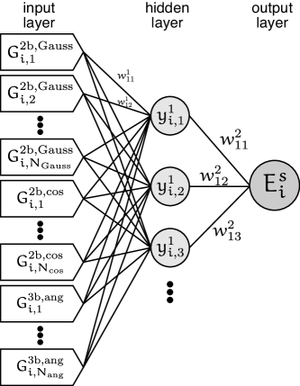
Figure 1: The structure of 1-hidden-layer NN model for Si system.

The weights in the NN potential $\{w\}$ are optimized through minimizing the following function,

$$\mathcal{L}(\{w\}) = \frac{1}{N_{s}}\sum_{s}\left[\left(\frac{E^{s,{\rm NN}}-E^{s,{\rm DFT}}}{N^{s}_{\rm a}}\right)^{2}\right.$$ (8)

$$+ \left.\frac{\kappa}{3N^{s}_{\rm a}}\sum_{i}^{N^{s}_{\rm a}}\sum_{\alpha}^{x,y,z}\left(F_{i,\alpha}^{s,{\rm NN}}-F_{i,\alpha}^{s,{\rm DFT}}\right)^{2}\right],$$

where $E^{s,{\rm DFT}}$ and $E^{s,{\rm NN}}=\sum_{i}E^{s,{\rm NN}}_{i}$ is the cohesive energies of a structure-$s$ obtained via DFT and NN-potential calculations; $F^{\rm s,DFT}_{i,\alpha}$ and $F_{i,\alpha}^{s,{\rm NN}}$ are the $\alpha$-components of forces on atom-$i$ in the structure-$s$ obtained via DFT and NN-potential calculations. $N^{s}_{\rm a}$ is the number of atoms in a structure-$s$, and $N_{s}$ is the number of samples considered. The parameter $\kappa$ is the conversion factor for forces that absorbs the difference of units between energy (eV) and force (eV/Å); it is set 0.05, which makes the force value 0.2 eV/Å correspond to the energy value 0.01 eV. The force term is important if the potential is applied to some dynamics simulation.Ercolessi and Adams (1994)

In order to select relevant and small number of bases, we adopt the FS regression approach.Hastie et al. (2001) The FS regression in this study proceeds as follows:

1. Weights on lines connecting bases and 1st layer nodes $\{w^{1}\}$ are set zero and other weights are set non-zero. Hence the weights to be optimized, $\{w\}_{\rm o}$, include only $\{w^{2}\}$ at this point.

2. Compute the sum of squared gradients associated to $\{w^{1}\}$,

   $$g^{\rm type}_{n}\equiv\sum_{m}\left(\frac{\partial\mathcal{L}}{\partial w^{1}_{mn\in{\rm type}}}\right)^{2},$$ (9)

   and find the largest one $g^{\rm max}_{n}$.

3. Append the weights, $\{w^{1}_{mn\in{\rm max}}\}$, which is related to the basis just selected in the previous step, to the weight set to be optimized, $\{w\}_{\rm o}$.

4. Perform the minimization with respect to the current weight set $\{w\}_{\rm o}$ until the convergence criterion, $|\mathcal{L}^{m}-\mathcal{L}^{m-1}|/|\mathcal{L}^{m-1}|<\varepsilon_{\rm tol}$, is achieved or the iteration $m$ exceeds the maximum iteration number $M$, where $\mathcal{L}^{m}$ is the $\mathcal{L}$ value at $m$-th iteration.

5. Go back to 2 unless all the bases are selected.

The number of iterations $M$ in the minimization at the step 4 should be large enough to find the minimum or at least the basin of the minimum in the $\{w\}_{\rm o}$-space. However, since large $M$ results in a lot of computation time for the iteration of the outer loop, $M$ or the convergence criterion for the minimization is usually set moderate value determined empirically. Since the FS regression searches the minimum near the origin of parameter space $\{w^{1}\}$ starting from the origin $w^{1}_{mn}=0$, over-fitting can be suppressed and a sparse NN model can be obtained as same as the LASSO. The FS regression has an advantage against the LASSO with regard to the computational cost of minimization, since the FS does not need to evaluate gradients of all weights but only the weights to be optimized $\{w\}_{\rm o}$ during the inner minimization loop, whereas the LASSO needs the gradients of all the weights. We can select the important bases that appears earlier than the other ones.

The sample structures prepared in this work were chosen so that the NN potential can well reproduce the crystalline and amorphous Si structures, some defect formation energies, and dynamical properties of liquid Si The samples include: perfect crystalline Si of some different crystal structure, such as diamond, fcc, bcc, and hcp; crystalline structure which involves a Si vacancy; generalized stacking faults on (111) plane of diamond structure; and uniform deformation, shear deformation, and random atom displacements of above mentioned structures; and liquid Si structures extracted from ab-initio MD simulation runs. We prepare 3930 samples that include 3930 energies and 90096 force components. The samples are divided into training-set data and test-set data, and the training-set data are used to optimize the NN and the test-set data are used to evaluate the NN potential. In this paper, randomly selected 10 % of all the samples are chosen as test samples.

To obtain the reference values, we adopt the DFT calculation using vasp (Vienna Ab-initio Simulation Package).Kresse and Furthmuller (1996); Kresse and Joubert (1999) The generalized gradient approximation (GGA) functionalPerdew et al. (1996) for the exchange-correlation potential and the projector augmented wave (PAW) methodBlöchl (1994) for the pseudo-potential of Si are adopted. The energy cutoff of expansion of plane waves is 250 eV. Phonon dispersion relations are calculated using phonopy.Togo et al. (2008) Molecular statics and MD calculations of liquid Si with NN potential are performed using our own code, nap (Nagoya Atomistic simulation Package).NAP (2015) (Nagoya Atomistic-simulation Package)

III Results and discussion

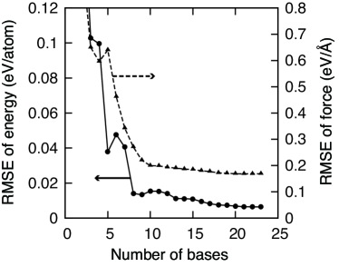
Figure 2: RMSEs of energy and force of test set as functions of number of bases extracted through the FS regression.

Relevant bases for crystalline and liquid Si system are selected using the FS regression as follows. The cutoff radius $r_{\rm c}$ and the number of nodes in a hidden layer are set 4.0 Å  and 10, respectively, according to the previous studiesBehler and Parrinello (2007); Behler (2011) and preliminary calculations. We prepare 300 bases including Gaussian, cosine, and angular types as $(N_{\rm Gauss},N_{\rm cos},N_{\rm ang})=(100,100,100)$. The number of iterations in the inner minimization, $M$, at the step 4 of the FS regression is 200. During the FS regression, the root mean squared errors (RMSEs) of energy and force for test set decrease as the number of bases increases as shown in Fig. 2. Eighteen bases are chosen since the RMSE of energy is less than 10 meV/atom. The selected bases include four Gaussian bases with $\{\eta\}=$ {0.1796, 0.4184, 1.0551, 1.9306}[${\rm\AA^{-2}}$], eleven cosine bases with $\{\xi\}=$ {0.7854, 0.8816, 1.1701, 1.4105, 1.7471, 2.4684, 2.6607, 2.8050, 2.8531, 2.9493, 3.1416}[${\rm\AA^{-1}}$], and three angular bases with $\{\lambda\}=$ {0.0, 0.6327, 1.0}. Then, the weights $\{w\}$ of these 18 bases are fully optimized within the space of selected bases. Final values of RMSE of energy and force obtained via the minimization are 3.9 meV/atom and 173 meV/Å, respectively. Figure 3 shows the relation between energies of samples obtained using NN potential and DFT. We can see that the NN potential with reduced number of bases well reproduces the DFT energies over a wide variety of structures.

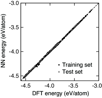
Figure 3: Relation between NN energies and DFT energies of sample data set. Energies about training set (filled circle) and test set (open triangle) are mostly on the ideal line.

It is worth looking into the NN structure in detail to understand how the NN potential works with selected bases. There are three angular bases selected through the FS regression. However, the $\lambda=1/3$, which corresponds to the bond angle of diamond Si and is adopted in the SW potential, is not included in the selected bases. The angular basis with $\lambda=1/3$ can be expanded with bases using $\lambda=0,\ 2/3,\ \text{and}\ 1$, as

$$\left(\cos\theta+\frac{1}{3}\right)^{2}=\frac{1}{3}(\cos\theta+0)^{2}+\left(\cos\theta+\frac{2}{3}\right)^{2}-\frac{1}{3}(\cos\theta+1)^{2}.$$ (10)

Thus one may think that the selected three bases of $\{\lambda\}=\{0.0,0.6327,1.0\}$ are just a reducible form of the basis with $\lambda=1/3$. However, seeing Fig. 4, which shows the weights from the three angular bases in the NN structure, the three bases contribute to nodes in the hidden layer in many ways, not like Eq. (10). Moreover, the nodes in the hidden layer receive contributions not only from angular bases but also from two-body bases, and the energy of an atom-$i$ is obtained from a weighted sum of these node values as in Eq. (1). Therefore, it is difficult to know which bases are important and to determine the number of bases heuristically.

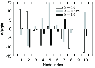
Figure 4: Weights from angular terms to nodes in the hidden layer, $\{w^{1}_{mn\in{\rm ang}}\}$. White, gray, and black bins indicate the weights from the angular bases with $\lambda=0.0$, 0.6327, and 1.0, respectively.

Elastic properties of Si diamond crystal obtained using the DFT, present NN potential, and SW potential are listed in Table 1. The NN potential reproduces elastic properties mostly within 10%; the lattice constant $a_{0}$, bulk modulus $B$, and a component of elastic constants $C_{11}$ are in good agreement. However, $C_{12}$ and $C_{44}$ differ slightly from the reference values, since the corresponding deformation modes for them are not included in the sample set. If we add some structures relevant to deformation modes to the training set, the potential could be improved. Figure 5 shows the phonon dispersion relations of the NN potential, DFT, and SW potential. The NN potential reproduces the phonon dispersion of DFT mostly better than SW potential. However, transversal acoustic branches of NN at the Brillouin zone edge are not good agreement with those of DFT. This can also be attributed to the lack of relevant structures in sample data set, and the NN potential cannot well extrapolate energies or forces of such deformation modes.

Table 1: Elastic properties of diamond Si, such as lattice constant $a_{0}$, cohesive energy $E_{\rm coh}$, bulk modulus $B$, elastic constants $C_{11}$, $C_{12}$, and $C_{44}$ calculated using DFT, SW potential, and NN potential.

	DFT	SW	NN
$a_{0}$ (${\rm\AA}$)	5.474	5.431	5.476
$E_{\rm coh}$ (eV/atom)	-4.541	-4.336	-4.537
$B$ (GPa)	88.31	101.38	84.08
$C_{11}$ (GPa)	168.0	149.8	165.1
$C_{12}$ (GPa)	77.4	74.8	64.4
$C_{44}$ (GPa)	95.4	109.7	86.3

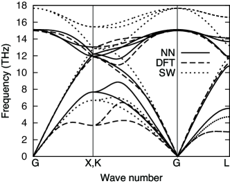
Figure 5: Phonon dispersion relations of DFT, SW, and NN. NN potential reproduces DFT phonon dispersion better than SW potential.

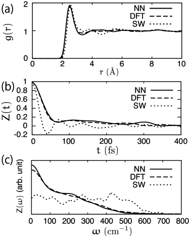
Figure 6: (a) Radial distribution function $g(r)$, (b) velocity autocorrelation function $Z(t)$, and (c) its power spectrum $Z(\omega)$, of liquid-Si at 2,000 K. NN well reproduces DFT results compared to SW.

The static and dynamic properties of liquid Si are also examined and compared between the NN, DFT, and SW, since it is known that the SW and Tersoff potentials do not well reproduce the dynamic properties of liquid Si obtained by the DFT.Ishimaru et al. (1996); Stich et al. (1996) Liquid structures and properties are obtained through MD simulation runs at 2,000K with about 7% larger density than that of the equilibrium diamond crystal at 0K.Stich et al. (1996) Figures 6(a), 6(b), and 6(c) show the radial distribution functions $g(r)$, velocity autocorrelation functions $Z(t)$, and their power spectra $Z(\omega)$, respectively. In all cases, the NN potential reproduces DFT results well, whereas the SW potential does not especially in $Z(t)$ and $Z(\omega)$. Especially, on the self diffusion, which can be estimated from the $Z(\omega=0)$, the NN potential well reproduces DFT result much better than the SW. This dynamic property of liquid Si is not well reproduced if the force data are not included in the function to be minimized unlike in Eq. (8). Hence the force-matching is necessary when we create potentials for the purpose of dynamics simulation.

IV Conclusion

We have constructed the neural-network (NN) interatomic potential for Si system with 18 bases selected from original 300 bases through the forward stepwise (FS) regression. The FS regression technique, which is similar to the sparsification by the least absolute shrinkage and selection operator (LASSO), allows us to extract important bases for the system considered. This approach can be straightforwardly applicable to any compound systems and enable us to create accurate and fast NN potentials. The present NN potential shows good agreements with DFT results such as elastic properties and phonon dispersion relation of crystalline Si, and static and dynamic properties of liquid Si. Thus it can be used for a variety of situations such as melting, amorphization, crystallization, and mechanical deformation of Si crystal.

References

- Matsumoto et al. (2002) M. Matsumoto, S. Saito, and I. Ohmine, Nature 416, 409 (2002).
- Henriksson et al. (2006) K. O. E. Henriksson, K. Nordlund, J. Keinonen, and J. Keinonen, Nuclear Instruments and Methods in Physics Research Section B: Beam Interactions with Materials and Atoms 244, 377 (2006).
- Hattori et al. (2015) R. Kobayashi, T. Hattori, T. Tamura, and S. Ogata, Journal of Nuclear Materials 463, 1071 (2015).
- Donnelly et al. (2013) G. Greaves, J. a. Hinks, P. Busby, N. J. Mellors, A. Ilinov, a. Kuronen, K. Nordlund, S. E. Donnelly, et al., Physical Review Letters 111, 065504 (2013).
- Jalem et al. (2013) R. Jalem, Y. Yamamoto, H. Shiiba, M. Nakayama, H. Munakata, T. Kasuga, and K. Kanamura, Chemistry of Materials 25, 425 (2013).
- Tanaka et al. (2015) K. Tanaka, S. Ogata, T. Tamura, and T. Kouno, International Journal of Heat and Mass Transfer 89, 714 (2015).
- Otani and Sugino (2006) M. Otani and O. Sugino, Physical Review B 73, 115407 (2006).
- Heyden et al. (2005) A. Heyden, A. T. Bell, and F. J. Keil, The Journal of Chemical Physics 123, 224101 (2005).
- Carlsson (1990) A. E. Carlsson, in Solid State Physics: Advances in Research and Applications, edited by H. Ehrenreich and D. Turnbull (Academic, New York, 1990), p. 1.
- Behler and Parrinello (2007) J. Behler and M. Parrinello, Physical Review Letters 98, 146401 (2007).
- Behler et al. (2008a) J. Behler, R. Martoňák, D. Donadio, and M. Parrinello, Physical Review Letters 100, 185501 (2008a).
- Behler et al. (2008b) J. Behler, R. Martoňák, D. Donadio, and M. Parrinello, physica status solidi (b) 245, 2618 (2008b).
- Behler (2011) J. Behler, The Journal of Chemical Physics 134, 074106 (2011).
- Artrith et al. (2011) N. Artrith, T. Morawietz, and J. Behler, Physical Review B 83, 153101 (2011).
- Artrith et al. (2012) N. Artrith, B. Hiller, and J. Behler, physica status solidi (b) 250, 1191 (2012).
- Sosso et al. (2012) G. C. Sosso, G. Miceli, S. Caravati, J. Behler, and M. Bernasconi, Physical Review B 85, 174103 (2012).
- Artrith and Behler (2012) N. Artrith and J. Behler, Physical Review B 85, 045439 (2012).
- Morawietz and Behler (2013) T. Morawietz and J. Behler, The Journal of Physical Chemistry A 117, 7356 (2013).
- Bartók et al. (2010) A. P. Bartók, M. C. Payne, R. Kondor, and G. Csányi, Physical Review Letters 104, 136403 (2010).
- Seko et al. (2014) A. Seko, A. Takahashi, and I. Tanaka, Physical Review B 90, 024101 (2014).
- Albe et al. (2002) K. Albe, K. Nordlund, and R. Averback, Physical Review B 65, 195124 (2002).
- Justo et al. (1998) J. F. Justo, M. Z. Bazant, E. Kaxiras, V. V. Bulatov, and S. Yip, Physical Review B 58, 2539 (1998).
- Hastie et al. (2001) T. Hastie, R. Tibshirani, and J. Friedman, The elements of statistical learning: data mining, inference and prediction (New York: Springer-Verlag, 2001).
- Stillinger and Weber (1985) F. H. Stillinger and T. A. Weber, Physical Review B 31, 5262 (1985).
- Pizzagalli et al. (2013) L. Pizzagalli, J. Godet, J. Guénolé, S. Brochard, E. Holmstrom, K. Nordlund, and T. Albaret, Journal of Physics: Condensed Matter 25, 055801 (2013).
- Tersoff (1988a) J. Tersoff, Physical Review B 38, 9902 (1988a).
- Tersoff (1988b) J. Tersoff, Physical Review B 37, 6991 (1988b).
- Ishimaru et al. (1996) M. Ishimaru, K. Yoshida, and T. Motooka, Physical Review B 53, 7176 (1996).
- Stich et al. (1996) I. Stich, M. Parrinello, and J. M. Holender, Physical Review Letters 76, 2077 (1996).
- Ercolessi and Adams (1994) F. Ercolessi and J. B. Adams, Europhysics Letters 26, 583 (1994).
- Kresse and Furthmuller (1996) G. Kresse and J. Furthmuller, Physical Review B 54, 11169 (1996).
- Kresse and Joubert (1999) G. Kresse and D. Joubert, 59, 11 (1999).
- Perdew et al. (1996) J. P. Perdew, K. Burke, and M. Ernzerhof, Physical Review Letters 77, 3865 (1996).
- Blöchl (1994) P. E. Blöchl, Physical Review B 50, 17953 (1994).
- Togo et al. (2008) A. Togo, F. Oba, and I. Tanaka, Physical Review B 78, 134106 (2008).
- NAP (2015) (Nagoya Atomistic-simulation Package) R. Kobayashi, computer code nap (Nagoya Atomistic-simulation Package), URL https://github.com/ryokbys/nap. The parameter set for the Si potential created in this paper is provided in the package.