Ultrafast Optimal Sideband Cooling under Non-Markovian Evolution

Abstract

A sideband cooling strategy that incorporates (i) the dynamics induced by structured (non-Markovian) environments in the target and auxiliary systems and (ii) the optimally-time-modulated interaction between them is developed. For the context of cavity optomechanics, when non-Markovian dynamics are considered in the target system, ground state cooling is reached at much faster rates and at much lower phonon occupation number than previously reported. In contrast to similar current strategies, ground state cooling is reached here for coupling-strength rates that are experimentally accesible for the state-of-the-art implementations. After the ultrafast optimal-ground-state-cooling protocol is accomplished, an additional optimal control strategy is considered to maintain the phonon number as closer as possible to the one obtained in the cooling procedure. Contrary to the conventional expectation, when non-Markovian dynamics are considered in the auxiliary system, the efficiency of the cooling protocol is undermined.

Introduction.—Fabricating and controlling micro- and nano-devices is of primary importance to develop quantum technologies. In this effort, optomechanical devices play a central role because they may become a building block for hybrid systems Mancini et al. (1998); Marquardt et al. (2007); Machnes et al. (2012); Aspelmeyer et al. (2014). To benefit from quantum effects, potential quantum technologies that utilize optomechanical systems need to prepare the mechanical component in the ground state. Thus, searching alternative schemes and refining present strategies to improve cooling protocols are of great interest. However, the highly non-trivial interplay between time-dependent external fields and structured environments poses constraints on the coherent control of these systems Schmidt et al. (2011) that have been barely explored.

Despite the copious recent literature on optomechanical cooling Mancini et al. (1998); Marquardt et al. (2007); Machnes et al. (2012); Marquardt and Girvin (2009); Wilson-Rae et al. (2007); Wang et al. (2011); Chan et al. (2011); Safavi-Naeini et al. (2013); Liu et al. (2013, 2015), a key point of the physics at low temperature remains unexplored, namely, low temperature induces non-Markovian dynamics Weiss (2012); Pachón and Brumer (2014); Pachón et al. (2014); Estrada and Pachon (2015). This very fact and the recent experimental evidence that the dynamics of micro-resonators are non-Markovian Groblacher et al. (2015), certainly, suggest that the present understating of cooling processes is incomplete. Moreover, because these approaches work on very short time-scales, of the order of the period of the resonator, it is expected that non-Markovian effects, either from low-temperature fluctuations or structured environments, dominate the energy and entropy transfer.

The exploration of non-Markovian dynamics has already leaded to the enhancement of, e.g., quantum speed limits Deffner and Lutz (2013), survival of entanglement Thorwart et al. (2009); Huelga et al. (2012); Estrada and Pachon (2015), improvements in quantum metrology Chin et al. (2012) and corrections to thermal equilibrium states Pachón et al. (2014); Yang et al. (2014). In the context of cooling, it was even shown that only under non-Markovian dynamics the entropy of a parametrically driven resonator can decrease Schmidt et al. (2011). The non-Markovian aspects of the dynamics discussed above are introduced here to one of the most promising techniques to reach the minimum phonon number, namely, finding an optimal coupling function via optimal control theory Schmidt et al. (2011); Wang et al. (2011). Based on analytic exact results derived in the context of the Feynman-Vernon influence theory, it is found that when the non-Markovian character is considered in the target resonator, the phonon number is lower than the predicted by Markovian processes; however, in contrast to the conventional expectation, non-Markovian dynamics in the auxiliary system deteriorates the cooling protocol.

Model and Theory.—For mechanical systems, sideband cooling consists in coupling a resonator to a microwave or optical resonator whose frequency is sufficiently high that it effectively sits in its ground state at ambient temperature. The coupling between the mechanical and electromagnetic modes is mediated by radiation pressure and is nonlinear. However, under realistic experimental conditions Teufel et al. (2011); Chan et al. (2011); Gigan et al. (2006); Kleckner and Bouwmeester (2006), the coupling can be assumed to be linear Marquardt et al. (2007); Aspelmeyer et al. (2014). This common model with linear coupling is considered below . Specifically, in the linear approximation, the system consists in two harmonic modes that describe the mechanical mode and the optical mode with the annhiqulation operators $\hat{a}$ and $\hat{b}$, respectively. The Hamiltonian reads

$$\hat{H}=\hbar{\omega_{\mathrm{mm}}}\hat{a}^{\dagger}\hat{a}+\hbar{\omega_{\mathrm{om}}}\hat{b}^{\dagger}\hat{b}+\hbar g(t)(\hat{a}^{\dagger}+\hat{a})(\hat{b}^{\dagger}+\hat{b})$$ (1)

with $\omega_{\mathrm{mm}}$ and $\omega_{\mathrm{om}}$, the frequency of the mechanical and electromagnetic modes, respectively, and $g(t)$ is the arbitrary time-dependent optomechanical coupling function to be found via optimal control theory Kirk (2012). For later convenience, the period of the mechanical mode is labeled by $\tau_{\mathrm{mm}}=2\pi/\omega_{\mathrm{mm}}$. To describe the interaction with the environment of the resonator and the losses in the cavity, each mode is coupled to an independent thermal bath with arbitrary spectrum and described in the context of the Ullersma-Caldeira-Leggett model Ullersma (1966); Caldeira and Leggett (1981) [see the Supplementary Material for details].

The particular functional form of the Hamiltonian (1), the environment model and the thermal initial states allow for the complete description of the dynamics in terms of the variances of the modes’ coordinates (see, e.g., Ref. Estrada and Pachon (2015)). This was utilized to combine sideband cooling and optimal control theory Wang et al. (2011). Specifically, the dynamics were formulated in terms of an adjoint master equation for the quadratures of the modes derived from the Markovian version of the Brownian-motion master equation Clerk et al. (2010); Gardiner and Zoller (2004). However, this master equation may violate the density-operator positivity (see Sec. 3.6 in Ref. Breuer and Petruccione (2007)). Moreover, for time dependent Hamiltonians, an adjoint Lindblad master equation can be derived only if the Liouvillian of the non-unitary dynamics commutes with its associated-time-ordered propagator (see Sec. 3.2 in Ref. Breuer and Petruccione (2007)), this is not the case for the Hamiltonian (1).

To circumvent the issues raised above, the Feynman-Vernon’s influence functional theory Feynman and Hibbs (2012) is employed here. It allows for performing a description of the dynamics without any approximation [see Supplementary Material]. and it further obeys the positivity of the density operator and straightforwardly incorporates driving fields. By combining the exact analytic results provided by the influence functional approach and an efficient numeral algorithm to solve integro-differential equations, the dynamics are solved here for arbitrary bath spectrum and driving field.

Non-Markovian Optimal Sideband Cooling.—The potential benefits from cooling optomechanical systems have attracted a great deal of attention Teufel et al. (2011); Marquardt et al. (2007); Genes et al. (2008); Wilson-Rae et al. (2007); Safavi-Naeini et al. (2013); Rivière et al. (2011); Mancini et al. (1998) and recently, it has been powered by optimal control theory Machnes et al. (2012); Wang et al. (2011). However, a key dynamical feature has been left out of the discussion, namely, the non-Markovian dynamics induced by low temperature and structured environments Weiss (2012); Pachón and Brumer (2014); Pachón et al. (2014); Estrada and Pachon (2015). Therefore, the goal here is to calculate and investigate the dependence of the minimum phonon number in the mechanical resonator $\langle\hat{n}\rangle(t_{\mathrm{cool}})$, at the shortest possible time $t_{\mathrm{cool}}$, on the non-Markovian character of the dynamics. In terms of the second moments of the position $\langle\hat{q}^{2}\rangle$ and momentum $\langle\hat{p}^{2}\rangle$, the phonon number at time $t$ is given by

$$\langle\hat{n}\rangle(t)=\frac{1}{2\hbar\omega}\left[\frac{\langle\hat{p}^{2}\rangle(t)}{m}+m{\omega_{\mathrm{mm}}}^{2}\langle\hat{q}^{2}\rangle(t)\right]-\frac{1}{2}.$$ (2)

The optimization procedure under non-Markovian dynamics, described in the Supplementary Material, leads to the minimum number phonon occupation at time $t_{\mathrm{cool}}$. The cooling time $t_{\mathrm{cool}}$ is chosen as short as possible by hand. The spectrum of the mechanical-resonator’s environment is described by the spectral density $J_{\mathrm{mm}}(\omega)=\gamma\omega_{\mathrm{D}}^{2}/\left(\omega_{\mathrm{D}}^{2}+\omega^{2}\right)$ whereas the cavity environment is chosen, for convenience, as $J_{\mathrm{om}}(\omega)=\kappa\Omega_{\mathrm{D}}^{2}/\left(\Omega_{\mathrm{D}}^{2}+\omega^{2}\right)$. As in Ref. Wang et al. (2011), it is assumed that the frequency conversion is exact and set $\omega_{\mathrm{mm}}=\omega_{\mathrm{om}}$. The corrections to this approximation are of the order of $\left(\omega_{\mathrm{mm}}/\omega_{\mathrm{om}}\right)^{2}$ This spectral density relates to temperature fluctuations CR02.

For typical values of optomechanical setups, Fig. 1(a) shows the optimal dynamics of the phonon number in the Markovian (dashed lines) and in non-Markovian (continuous lines) regime. Figure 1 shows two alternatives to decrease the minimum phonon number, namely, (i) extending the cooling time or (ii) considering non-Markovian effects in the dynamics. By lengthening the cooling process from $t_{\mathrm{cool}}=0.55\tau_{\mathrm{m}}$ (black and cyan lines) to $t_{\mathrm{cool}}=1.25\tau_{\mathrm{m}}$ (green and magenta lines) and for the initials phonon number in the mechanical mode $n_{\mathrm{T}}=10^{2}$ and $n_{\mathrm{T}}=10^{3}$, it is possible to decrease the minimum phonon number by an order of magnitude, from ca. $\langle n(t_{\mathrm{cool}})\rangle=10^{-2}$ to $\langle n(t_{\mathrm{cool}})\rangle=10^{-3}$. The Markovian and non-Markovian character of the dynamics does not change considerably the functional form of the optomechancal coupling; however, the small difference is enough to decrease the minimum phonon-number by around one order of magnitude (see also Table 1).

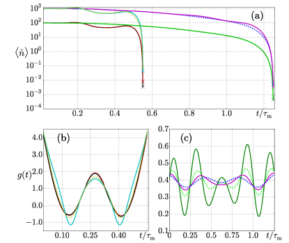
Figure 1: (a) Time evolution of the phonon number $\hat{n}(t)$ during the optimal modulation of the interaction with $n_{\mathrm{c}}=0$, $\gamma=10^{-6}\omega_{\mathrm{m}}$ and $\kappa=2.15\times 10^{-4}\omega_{\mathrm{m}}$. In particular, for $n_{\mathrm{T}}=10^{2}$ ($n_{\mathrm{T}}=10^{3}$) and final time $t_{\mathrm{cool}}=0.55\tau_{\mathrm{m}}$ ($t_{\mathrm{cool}}=1.25\tau_{\mathrm{m}}$), the dashed red (blue) curve depicts the dynamics of the phonon number under Markovian dynamics ($\omega_{\mathrm{D}}=\Omega_{\mathrm{D}}=100\omega_{\mathrm{m}}$) while the continuos black (magenta) curve depicts the dynamics under non-Markovian dynamics ($\omega_{\mathrm{D}}=\Omega_{\mathrm{D}}=\omega_{\mathrm{m}}$). The continuos dark green (cyan) curve depicts the non-Markovian phonon-occupation-number dynamics for $n_{\mathrm{T}}=10^{2}$ ($n_{\mathrm{T}}=10^{3}$) and $t_{\mathrm{cool}}=1.25\tau_{\mathrm{m}}$ ($t_{\mathrm{cool}}=0.55\tau_{\mathrm{m}}$) whereas the dashed olive (light green) curve stands for the Markovian dynamics. The $y$-axis is in logarithmic scale. (b) Optimal coupling function with $t_{\mathrm{cool}}=0.55\tau_{\mathrm{m}}$ under non-Markovian (continuous lines) and Markovian dynamics (dashed line). (c) Optimal coupling function with $t_{\mathrm{cool}}=1.25\tau_{\mathrm{m}}$ under non-Markovian (continuous lines) and Markovian dynamics (dashed line).

	$\langle\hat{n}(t_{\mathrm{cool}})\rangle$
$\gamma/\omega_{\mathrm{m}}$	opt. om${}_{\mathrm{M}}+$ mmM	om${}_{\mathrm{nM}}+$ mmnM	opt. om${}_{\mathrm{nM}}+$ mmnM	om${}_{\mathrm{M}}+$ mmnM	opt. om${}_{\mathrm{M}}+$ mmnM
$10^{-6}$	$9.03\times 10^{-3}$	8.86$\times 10^{-3}$	3.43$\times 10^{-3}$	1.91$\times 10^{-3}$	9.99$\times 10^{-5}$
$10^{-5}$	$1.04\times 10^{-2}$	1.02$\times 10^{-2}$	4.79$\times 10^{-3}$	2.60$\times 10^{-3}$	7.91$\times 10^{-4}$
$10^{-4}$	$3.28\times 10^{-2}$	2.40$\times 10^{-2}$	1.99$\times 10^{-2}$	1.63$\times 10^{-2}$	1.52$\times 10^{-2}$
$10^{-3}$	$2.61\times 10^{-1}$	1.61$\times 10^{-1}$	1.53$\times 10^{-1}$	1.53$\times 10^{-1}$	1.51$\times 10^{-1}$
$10^{-2}$	$2.45$	1.52	1.50	1.50	1.50
$10^{-1}$	$21.12$	14.21	13.52	13.52	13.52

Table 1: Minimum phonon number in the mechanical resonator at a time $t_{\mathrm{cool}}=0.55\tau_{\mathrm{m}}$ for different values of the dissipation rate $\gamma/\omega_{\mathrm{m}}$ and for different cooling scenarios (see text). Cavity dissipation rate $\kappa=10^{-4}\omega_{\mathrm{m}}$.

The coupling strength for the ultrafast cooling scenario in Fig. 1(b) is beyond the present experimental capabilities; however, results for the fast cooling case in Fig. 1(c) are encouraging Teufel et al. (2011). Moreover, in the regime of Fig. 1(c) cooling from room temperature is possible Liu et al. (2015).

The non-trivial interplay between non-Markovian dynamics and driving fields is explored in Table 1, it displays the predicted phonon number for a variety of scenarios, namely, (i: opt. om${}_{\mathrm{M}}+$ mm_M) the minimum phonon number obtained from optimization under Markovian dynamics, (ii: om${}_{\mathrm{nM}}+$ mm_nM) the phonon number obtained under non-Markovian dynamics with the optimal coupling found under Markovian dynamics, (iii: opt. om${}_{\mathrm{nM}}+$ mm_nM) the phonon number obtained from optimization under non-Markovian dynamics, (iv: om${}_{\mathrm{M}}+$ mm_nM) the phonon number obtained under Markovian dynamics in the optical mode and non-Markovian dynamics in the mechanical mode with the optimal coupling found under Markovian dynamics and (v: opt. om${}_{\mathrm{M}}+$ mm_nM) the phonon number obtained from optimization under Markovian dynamics in the optical mode and non-Markovian dynamics in the mechanical mode.

Comparison of scenarios (i) and (ii) in Table 1 shows that, for the same coupling function, the presence of non-Markovian dynamics reduces the minimum phonon number and that this decrease is more noticeable when the dissipation rate of the mechanical resonator increases. The third scenario depicts the influence of the optimization process. Even though there is a reduction in the phonon number respect to the second scenario, in absolute terms, the decrease is tiny. Besides, if the optical-mode dynamics are considered as Markovian and the dynamics of the mechanical mode as non-Markovian, fourth scenario, there is a decrease in the number of phonons for low values of the decay factor $\gamma/\omega_{\mathrm{m}}$. Surprisingly, only when Markovian, non-Markovian dynamics and optimal control theory are combined, fifth scenario, a substantial reduction in the phonon number is reached for low mechanical decay rates. For these low-decay-factor cases, which are relevant under experimental conditions, the strategy in the fifth scenario is able to bring the number of phonons more than one order of magnitud below the number of phonons reached under the conditions of the first scenario.

This non-trivial and unexpected interplay between Markovian, non-Markovian dynamics and optimal control theory is also observed for a variety of values of the cavity decay rate in Table 2. The advantage of a Markovian-dynamics cavity is more transparent for large values of the cavity losses rate $\kappa$, e.g., for a non-Markovian cavity ($\Omega_{\mathrm{D}}=\omega_{\mathrm{c}}$) with $\kappa=2.15\times 10^{-1}\omega_{\mathrm{c}}$, there is no ground-state cooling [$\langle\hat{n}_{\mathrm{nM}}(t_{\mathrm{cool}})=2.34$].

$t_{\mathrm{cool}}/\tau_{\mathrm{m}}$	$\kappa/\omega_{\mathrm{c}}$	$\langle\hat{n}_{\mathrm{M}}(t_{\mathrm{cool}})\rangle$	$\langle\hat{n}_{\mathrm{nM}}(t_{\mathrm{cool}})\rangle$	$\langle\hat{n}_{\mathrm{om_{M}}}(t_{\mathrm{cool}})\rangle$
0.55	1$\times 10^{-3}$	0.016	0.015	0.014
0.6	1.5$\times 10^{-2}$	0.025	0.019	0.019
0.8	2.5$\times 10^{-2}$	0.029	0.030	0.021
0.8	4.5$\times 10^{-2}$	0.035	0.060	0.026
0.8	5.5$\times 10^{-2}$	0.037	0.086	0.032
1.0	1.25$\times 10^{-1}$	0.048	0.356	0.040
1.6	2.15$\times 10^{-1}$	0.056	2.34	0.044

Table 2: Minimum phonon number for scenarios (i: opt. om${}_{\mathrm{M}}+$ mm_M) $\langle\hat{n}_{\mathrm{M}}(t_{\mathrm{cool}})$, (iii: opt. om${}_{\mathrm{M}}+$ mm_M) $\langle\hat{n}_{\mathrm{nM}}(t_{\mathrm{cool}})$ and (v: opt. om${}_{\mathrm{M}}+$ mm_M) $\langle\hat{n}_{\mathrm{om_{M}}}(t_{\mathrm{cool}})$ for different cooling times and for different parameters of cavity dissipation. The initial parameters are $n_{\mathrm{T}}=100$, $\gamma=10^{-4}\omega_{\mathrm{m}}$.

Because the mechanical-mode initial state is highly thermally-populated, the non-Markovian character of the dynamics originates mainly from the structure of the thermal bath and not from quantum fluctuations at low temperature. This explains why, for non-structured environments, Markovian descriptions of the dynamics may had provided sensible results.

Maintaining the minimum phonon number over time.—Reaching a very low phonon number in a short period of time is a desirable goal. However, because the resonator is continuously coupled to its environment, keeping that phonon number is a must. In doing so, introduce a second optimal control scenario where the objetive is to maintain, over a long period of time, the minimum number of phonons in the resonator reached in the ultrafast cooling in Fig. 1. Define then a composite optimal optomechanical coupling function as

$$c(t)=\left\{\begin{array}[]{l c}g_{\mathrm{c}}(t)&0\leq t\leq t_{\mathrm{cool}},\\ g_{\mathrm{m}}(t)&t>t_{\mathrm{cool}},\end{array}\right.$$ (3)

which encompasses the entire cooling process, i.e., reaching a minimum phonon number by applying $g_{\mathrm{c}}(t)$ and maintaining this number once it is obtained with $g_{\mathrm{m}}(t)$. Because performing the second optimization process under non-Markovian dynamics over long times requires an enormous amount of computing time, the second optimization process is performed under the assumption that for long times, the Markovian approximation holds so that the optimal coupling function is calculated for Markovian dynamics.

Figure 2(a) depicts the time evolution of the phonon number under the action of the optimal coupling function $c(t)$ for a variety of experimentally-relevant values of the decay rate $\gamma$. To obtain an experimentally-accessible-coupling-strength scenario, $|c(t)|<10^{-1}$, the cooling time is set to $t_{\mathrm{cool}}=6\tau_{\mathrm{m}}$ and the initial phonon number to $n_{\mathrm{T}}=10^{2}$ [see Fig. 2(b)]. For the second control phase, the initial number of phonons is set to be the minimum phonon number reached at $t_{\mathrm{cool}}$. To maintaining the minimum phonon number requires moving from the strong coupling regime to a weak coupling regime between the two modes, see Figs. 2(b) and 2(c). Likewise, with the optimal optomechanical coupling function $c(t)$ the phonon number is approximately maintained for 50 periods of the mechanical resonator.

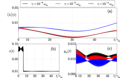
Figure 2: (a) Phonon number as a function of time during the optimal control protocol aimed at maintaing the minimum phonon number for different values of the dissipation rate. The initial parameters are $n_{\mathrm{T}}=\langle n(t_{\mathrm{cool}})\rangle$, $n_{\mathrm{c}}=0$, $\kappa=2.15\times 10^{-4}$. (b) The optimal optomechanical coupling function $c(t)$ for $\gamma=10^{-6}\omega_{\mathrm{m}}$. (c) The optimal optomechanical coupling function $g_{\mathrm{m}}(t)$.

Discussion.—Analytical solutions and an efficient optimal control protocol showed that the presence of non-Markovian dynamics allows for lower phonon numbers than the predicted by Markovian-and-RWA-based previous works. Surprisingly, significant enhancements are found as the interplay between non-Markovian dynamics in the mechanical mode, Markovian dynamics in optical mode and optimally-designed coupling functions. To understand this effect, note that for well-behaved $J(\omega)$, non-Markovian dynamics define an effective coupling to the thermal bath Pachón et al. (2014); Estrada and Pachon (2015) that, in general, is weaker than the Markovian one. Thus, when non-Markovian dynamics are considered in the cavity dynamics, the rate at which the electromagnetic mode releases the entropy, that absorbes from the mechanical mode, into its environment diminishes and therefore, the number of phonons in the mechanical mode does not largely decrease compared to the case of Markovian-dynamics cavity. Furthermore, because the mechanical mode is constantly coupled to its environment, the optimal cooling protocol was extended [see Eq. (3)] to preserve the phonon number as low as possible after cooling is reached. For this second protocol, the coupling amplitude is between reach of present technology and can be combined with already-experimentally-implemented cooling protocols Chan et al. (2011); Teufel et al. (2011); Gigan et al. (2006); Kleckner and Bouwmeester (2006).

The optimization protocol developed here relies on the optimization over the Green functions of the trajectories that minimize the influence functional (see Supplementary Material) and can be readily implemented in semiclassical formulations of quantum mechanics in phase space Pachón et al. (2010); Dittrich et al. (2010). Thus, non-linear systems can be addressed and the influence of quantum fluctuations in the design of optimal pulses of coupling functions can be analyzed. This enables the present proposal, e.g., in the context of optimal control theory of molecular processes Shapiro and Brumer (2012).

See pages 1 of SIoscprl.pdf

See pages 2 of SIoscprl.pdf

See pages 3 of SIoscprl.pdf

See pages 4 of SIoscprl.pdf

See pages 5 of SIoscprl.pdf

See pages 6 of SIoscprl.pdf

See pages 7 of SIoscprl.pdf

See pages 8 of SIoscprl.pdf

See pages 9 of SIoscprl.pdf

See pages 10 of SIoscprl.pdf

See pages 11 of SIoscprl.pdf

See pages 12 of SIoscprl.pdf

See pages 13 of SIoscprl.pdf

See pages 14 of SIoscprl.pdf

See pages 15 of SIoscprl.pdf

See pages 16 of SIoscprl.pdf

See pages 17 of SIoscprl.pdf

See pages 18 of SIoscprl.pdf

See pages 19 of SIoscprl.pdf

See pages 20 of SIoscprl.pdf

See pages 21 of SIoscprl.pdf

See pages 22 of SIoscprl.pdf

See pages 23 of SIoscprl.pdf

See pages 24 of SIoscprl.pdf

See pages 25 of SIoscprl.pdf

See pages 26 of SIoscprl.pdf

See pages 27 of SIoscprl.pdf

See pages 28 of SIoscprl.pdf

See pages 29 of SIoscprl.pdf

See pages 30 of SIoscprl.pdf

See pages 31 of SIoscprl.pdf

See pages 32 of SIoscprl.pdf

See pages 33 of SIoscprl.pdf

See pages 34 of SIoscprl.pdf

See pages 35 of SIoscprl.pdf

See pages 36 of SIoscprl.pdf

See pages 37 of SIoscprl.pdf

See pages 38 of SIoscprl.pdf

See pages 39 of SIoscprl.pdf

See pages 40 of SIoscprl.pdf

See pages 41 of SIoscprl.pdf

See pages 42 of SIoscprl.pdf

See pages 43 of SIoscprl.pdf

See pages 44 of SIoscprl.pdf

See pages 45 of SIoscprl.pdf

See pages 46 of SIoscprl.pdf

See pages 47 of SIoscprl.pdf

See pages 48 of SIoscprl.pdf

See pages 49 of SIoscprl.pdf

See pages 50 of SIoscprl.pdf