Breakdown of separability due to confinement

Abstract

A simple system of two particles in a bidimensional configurational space $S$ is studied. The possibility of breaking in $S$ the time independent Schrödinger equation of the system into two separated one-dimensional one-body Schrödinger equations is assumed. In this paper, we focus on how the latter property is countered by imposing such boundary conditions as confinement in a limited region of $S$ and/or restrictions on the joint coordinate probability density stemming from the sign-invariance condition of the relative coordinate (an impenetrability condition). Our investigation demonstrates the reducibility of the problem under scrutiny into that of a single particle living in a limited domain of its bidimensional configurational space. These general ideas are illustrated introducing the coordinates $X_{c}$ and $x$ of the center of mass of two particles and of the associated relative motion, respectively. The effects of the confinement and the impenetrability are then analyzed by studying with the help of an appropriate Green’s function and the time evolution of the covariance of $X_{c}$ and $x$. Moreover, to calculate the state of the single particle constrained within a square, a rhombus, a triangle and a rectangle the Green’s function expression in terms of Jacobi $\theta_{3}$-function is applied. All the results are illustrated by examples.

Keywords: Quantum boundary conditions, Confinement, Center of mass, Time evolution, Jacobi $\theta_{3}$-function.

1. Introduction

Over the decade, many papers appeared dedicated to the problem of quantum systems with boundaries. Several works are devoted to the problem of particles confined in a box, sometimes with moving walls [1, 2, 3, 4, 5, 6, 7] or specific shapes [8, 9]. The confinement means the restriction on the motion of randomly moving particles, e.g. by the potential barriers.

The confined systems have become a topical issue common to many research areas from condensed matter physics and quantum optics to biophysics. The first easy to understand reason is that today an accurate quantitative prediction of the physical behavior of such systems is required by experimentalists since they cannot ignore confinement effects when the spacial constraints stemming from the extreme miniaturization required for applications reach micro or nano-sizes. During the recent years some laboratory realization of new experimental systems like two and three dimensional graphite cones, carbon nano-tube rings [10, 11] and torus shaped nano-rings [12, 13] generated interest in the development of the idea of the quantum confinement. They can be used in development of nano and molecular electronic circuit devices. The second important reason is that the physical behavior of exemplary systems like a harmonic oscillator [14, 15, 16], an atom [17, 18, 19] or a small molecule, when subjected to such boundary conditions, may exhibit qualitative differences with respect to that available in the literature, for example, due to a breaking of the geometrical symmetry. This may lead to deep modifications on the eigensolutions of the system as well as to the need of a different way of treating the center of mass motion in the case of more than one particle in the system.

In this paper, we first elucidate the breakdown of the separability of the center of mass motion from their relative motion for an unidimensional system of two, even non interacting, particles stemming from the confinement of the system. To this end, we first analyze the ”traditional” confinement constraint consisting on limiting the motion of the two particles inside a finite and the same interval $I\subset\mathds{R}$. In addition to such a boundary condition we distinguish the case when the relative coordinate is allowed to assume both positive and negative values from that when one of two particles is always on the same side with respect to the other one. We refer to this last situation speaking of an ”impenetrability condition” describing it as an effective further constraint on the system. Recently unidimensional systems exhibiting this kind of restriction on the motion of the particles have been realized in laboratory [20]. Our target is to compare the separable motion of two totaly unconstrained particles, that is $I=\mathds{R}$ and the lack of impenetrability, with the ones when at least one out of the two constraints is instead present. Our results clearly illustrate that the existence of a basis of factorized stationary states of two even noninteracting quantum particles critically depends on whether and how the relevant dynamical variables get algebraically linked on the frontier of the bidimensional domain out of which any wave function compatible with the assumed constraints, vanish. In other words, we highlight that separability depends not only on the structure of the relative Schrödinger equation but also on the geometric shape of the normalization domain. This observation paves the way to the possibility of tracing back the confined motion of our unidimensional system of two noninteracting particles to that of a fictitious particle moving in a plane within a domain whose shape is determined by the restrictions imposed on our original two-particle system. The second part of this paper is thus dedicated to quantum billiards problems with plain domains as the square, the rhombus, the triangle and the rectangle. Also, the time evolution of the covariance of the center of mass coordinates is obtained. To this end, the theta-three Green’s function theory [21] is applied. It is worthy to mention that Jacobi $\theta_{3}$-function was used to study coherence states of a charge moving in constant magnetic field [22].

A quantum particle inside the potential of a special form is an interesting problem. There are many studies connected with the quantum and the classical properties of the bidimensional difficult geometries like, for example, the Robnik’s billiard and the Bunimovich’s stadium [23, 24], the Sinai’s billiard [25]. The quantum particle in the triangle potential is studied in [26, 27, 28, 29]. The triangular shaped potential appears in different contexts. For example, in the equipotential curves for the Hénon-Heiles system [30]. Inside the boundary the potential behaves like the bidimensional harmonic oscillator, but in the billiard case, the particle has a free motion inside the triangular shaped domain. The brief review on the triangular billiard geometry problems is given, for example, in [31].
In this paper, we study four different shapes of the potential. It is shown how using the known boundary conditions for the particle confined in the square box with the side $d$, the boundary conditions for the boxes forming the rhombus, the triangle and the rectangle are constructed. Moreover, the Green’s function using the Jacobi $\theta_{3}$-function for all four cases is obtained.

The paper is organized as follows. In Sec. 2. the case of two noninteracting particles confined in the unidimensional box is considered. The boundary conditions are written for the center of mass motion. The case of the presence of the impenetrability condition is discussed. In Sec. 3. the problem of the single free particle motion on the plane in the domain of the motion being restricted by the unpenetrated walls forming the square, the rhombus, the triangle (the triangle billiard) and the rectangle are studied. In Sec. 4. the time evolution of the wave function is obtained. The time evolution of the covariance of the center of mass coordinates is shown for the bounded and the unbounded problems. In Sec. 5. the Green’s function is used to find the time-dependent states for the covariance. The results obtained are illustrated on the example of the single particle motion confined in the square impenetrable box with the side $d$.

2. Two particles confined in a one-dimensional box

Let us consider a system of two particles with masses $m_{1}$ and $m_{2}$ confined in a one-dimensional box (tube) of a length $d$ delimited by two impenetrable walls. The coordinates of the first and the second particle are $0\leq x_{1}\leq d$ and $0\leq x_{2}\leq d$, respectively. The Schrödinger equation for the two noninteracting particles is the following

$$-\frac{\hbar^{2}}{2}\left(\frac{1}{m_{1}}\frac{\partial^{2}}{\partial x_{1}^{2}}+\frac{1}{m_{2}}\frac{\partial^{2}}{\partial x_{2}^{2}}\right)\Psi(x_{1},x_{2})=E\Psi(x_{1},x_{2}).$$ (1)

It is known that in general the solution of (1) is the following

$$\Psi_{free}(x_{1},x_{2})=(A\sin(k_{1}x_{1})+B\cos(k_{1}x_{1}))(C\sin(k_{2}x_{2})+D\cos(k_{2}x_{2})),$$ (2)

where $k_{i}=\sqrt{\frac{2m_{i}E}{\hbar^{2}}}$, $i=1,2$. The four constants $A,B,C,D$ must be determined taking into account normalization and the presence of the boundaries. In our case $\Psi_{free}(x_{1},x_{2})$ must vanish outside of the box and on the boundaries, that is

$$\Psi(x_{1}=0,x_{2})=\Psi(x_{1},x_{2}=0)=0,\quad\Psi(x_{1}=d,x_{2})=\Psi(x_{1},x_{2}=d)=0.$$ (3)

The solution (2) respecting such boundary conditions (3) can be hence rewritten as

$$\Psi_{conf}(x_{1},x_{2})=N\sin(k_{1}x_{1})\sin(k_{2}x_{2}),$$ (4)

where $k_{1}=\pi n_{1}/d$, $k_{2}=\pi n_{2}/d$, $N$ is the appropriate normalization constant.

Introducing the well known center of mass transformation

$$x=x_{1}-x_{2},\quad X_{c}=\frac{m_{1}x_{1}+m_{2}x_{2}}{M},\quad M=m_{1}+m_{2},\quad\mu=\frac{m_{1}m_{2}}{M},$$ (5)

one can rewrite (1) as

$$-\frac{\hbar^{2}}{2}\left(\frac{1}{\mu}\frac{\partial^{2}}{\partial x^{2}}+\frac{1}{M}\frac{\partial^{2}}{\partial X_{c}^{2}}\right)\widetilde{\Psi}(X_{c},x)=E\widetilde{\Psi}(X_{c},x).$$ (6)

For the problem of free particles this approach leads to the possibility of finding eigensolution of (6) in the form of a product, e.g. $\widetilde{\Psi}(X_{c},x)=\widetilde{\Psi}_{1}(X_{c})\widetilde{\Psi}_{2}(x)$.

The representation of (4) in terms (5) is the following

$$\widetilde{\Psi}_{conf}(X_{c},x) = -\widetilde{N}e^{-iX_{c}(k_{1}+k_{2})}e^{ix\frac{m_{2}k_{1}-m_{1}k_{2}}{M}}$$

$$\times \left(e^{2iX_{c}k_{1}}e^{-2ix\frac{m_{2}k_{1}}{M}}-1\right)\left(e^{2iX_{c}k_{2}}e^{2ix\frac{m_{1}k_{2}}{M}}-1\right),$$

where $\widetilde{N}$ is a normalization constant.

From (5) we can write that

$$x_{1} = X_{c}+\frac{m_{2}}{M}x,\quad x_{2}=X_{c}-\frac{m_{1}}{M}x,\quad 0\leq x_{1}\leq d,\quad 0\leq x_{2}\leq d.$$ (8)

Hence, in the plane $(X_{c},x)$ the domain of variability of $X_{c}$ and $x$ turn out to be bounded by the four lines shown in Fig. 1.

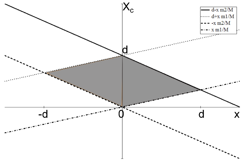
Fig. 1: The domain of $X_{c}$ and $x$.

Moreover, we can deduce the geometrical boundary conditions for the solution of (6) in the center of mass coordinates as

$$\widetilde{\Psi}\left(X_{c},x|X_{c}+\frac{m_{2}}{M}x=d\right)=0,\quad\widetilde{\Psi}\left(X_{c},x|X_{c}-\frac{m_{1}}{M}x=d\right)=0,$$ (9)

$$\widetilde{\Psi}\left(X_{c},x|X_{c}+\frac{m_{2}}{M}x=0\right)=0,\quad\widetilde{\Psi}\left(X_{c},x|X_{c}-\frac{m_{1}}{M}x=0\right)=0.$$

One should note that from the latter conditions the coordinates $X_{c}$ and $x$ are algebraically related in the frontier of the domain. Hence, in the presence of the boundary conditions the separation of the variables is impossible [32] and we can not look for the solution of (6) as a factorized function of the two variables. Thus (6) can not be rewritten in two differential equations and relative boundary conditions each one depending only on one variable. We conclude that in the presence of the boundary conditions (9) the problem (6) is not separable.

Let us search the solution of (6) in the form

$$\widetilde{\Psi}(X_{c},x) = (Ae^{\imath k1(aX_{c}+bx)}+Be^{-\imath k1(aX_{c}+bx)})(Ce^{\imath k2(cX_{c}+dx)}+De^{-\imath k2(cX_{c}+dx)}).$$

Using the boundary conditions (9), we get $a=c=1$, $A=C=1,B=D=-1$, $b=-m_{2}/M$, $d=m_{1}/M$ and $k_{1}=\pi n_{1}/d$, $k_{2}=\pi n_{2}/d$. Hence, the energy eigenvalues are

$$E_{n_{1}n_{2}}=\frac{\hbar^{2}k_{1}^{2}}{2m_{1}}+\frac{\hbar^{2}k_{2}^{2}}{2m_{2}}.$$

Thus, the solution of (6) with respect to the new geometric boundary conditions (9) is the following

$$\widetilde{\Psi}_{n_{1}n_{2}}(X_{c},x)\!\! = \!\!\widetilde{C}(e^{\imath\frac{\pi n_{1}}{d}(X_{c}+\frac{m_{2}}{M}x)}-e^{-\imath\frac{\pi n_{1}}{d}(X_{c}+\frac{m_{2}}{M}x)})(e^{\imath\frac{\pi n_{2}}{d}(X_{c}-\frac{m_{1}}{M}x)}-e^{-\imath\frac{\pi n_{2}}{d}(X_{c}-\frac{m_{1}}{M}x)})$$ (10)

$$= \widetilde{A}\sin\left(\frac{\pi n_{1}}{d}(X_{c}+\frac{m_{2}}{M}x)\right)\sin\left(\frac{\pi n_{2}}{d}(X_{c}-\frac{m_{1}}{M}x)\right),$$

that is (4) rewritten in the center of mass coordinates. The normalization constant can be found from normalization condition, rewritten in the notations (5). Namely

$$2\int\limits_{0}^{d}dx\left(\int\limits_{\frac{m_{1}x}{M}}^{d-\frac{m_{2}x}{M}}\Big{|}\widetilde{\Psi}_{n_{1}n_{2}}(X_{c},x)\Big{|}^{2}dX_{c}\right)=1$$

and the constant may be assumed to be equal to $\widetilde{A}=\frac{2}{d}$. If we assume that the crossection of the tubes possese a radius comparable with the liniar dimension of the particles, then they can not penetrate each other. Hence, we can think that the first particle is on the right hand side while the second one is on the left hand side of the box, e.g. $x_{1}>x_{2}$. Using this additional condition and (8) we can write

$$X_{c}+\frac{m_{2}}{M}x>X_{c}-\frac{m_{1}}{M}x.$$ (11)

Thus $x>0$ that is always true for the present system, where $0<x<d$. That means that the additional condition on the penetrability of the particles influences the boundary conditions for the center of mass motion and the new domain is shown in Fig.2. Note that (10) does not fullfill the latter geometric boundary condition.

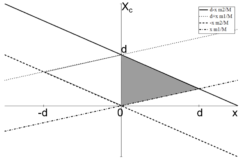
Fig. 2: The domain of $X_{c}$ and $x$ when the particles can not penetrate each other.

In the presence of the inpenetrability condition, e.g. $x_{1}>x_{2}$, but absence of the confinement (that means that $x_{1},x_{2}\in(-\infty,\infty)$) we can write (11) and get the condition analogues to confinement from the one boundary.

3. One particle confined in the two dimensional box

The problem of the two particles confined in the one dimensional box is equvivalent to the problem of one particle confined in the two dimensional box. The Schrödinger equation for such system is

$$-\frac{1}{2m}\left(\frac{\partial^{2}}{\partial x_{1}^{2}}+\frac{\partial^{2}}{\partial x_{2}^{2}}\right)\Phi(x_{1},x_{2})=E\Phi(x_{1},x_{2}).$$ (12)

Hence, in this section we study the the single free particle motion on the plane, but the domain of the motion being restricted by unpenetrated walls forming the the square with the side $d$, the rhombus with the side $d$, the triangle and the rectangle (see Fig. 3).

Let us start from the square impenetrable box with the side $d$. The solution of the Schrödinger equation (12) is

$$\Phi(x_{1},x_{2}) = A\sin(n_{1}x_{1})\sin(n_{2}x_{2}),$$ (13)

where $A$ is a normalization parameter. From the boundary conditions

$$\Phi(x_{1}=\pm d,x_{2})=\Phi(x_{1},x_{2}=\pm d)=0$$

we can estimate the parameters of the solution, ss. $n_{1}=\frac{\pi N_{1}}{d}$, $n_{2}=\frac{\pi N_{2}}{d}$, $N_{1},N_{2}=0,\pm 1,\pm 2,\ldots$.

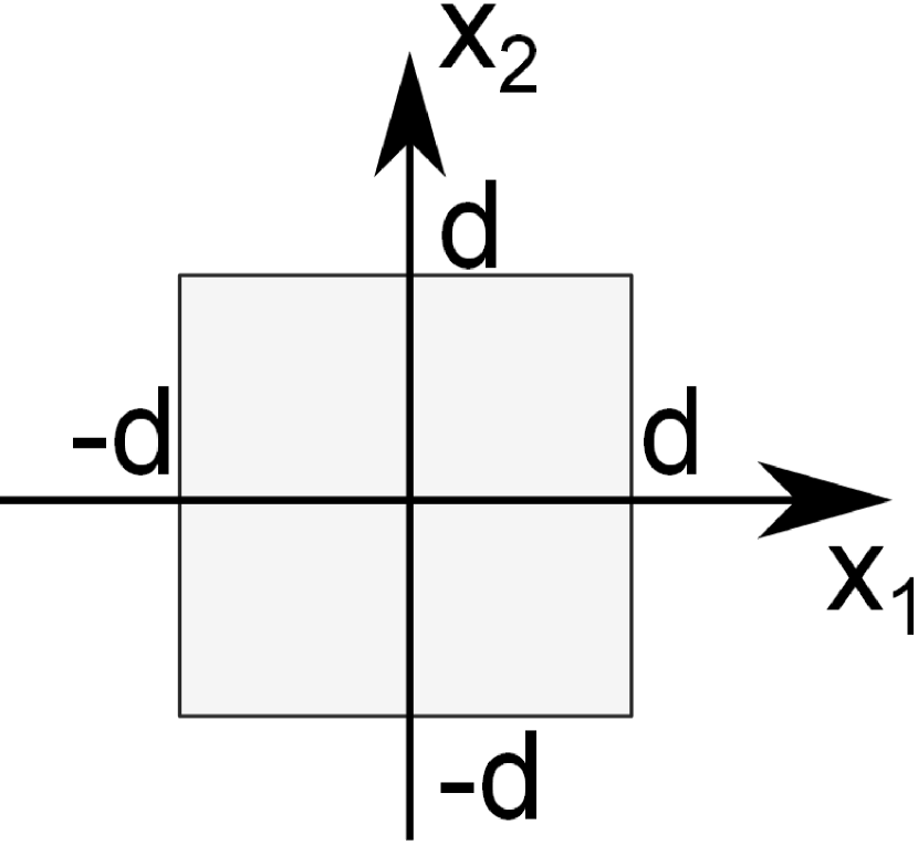
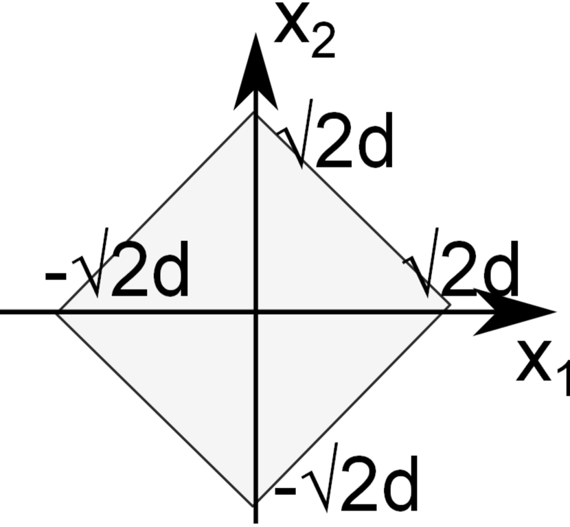
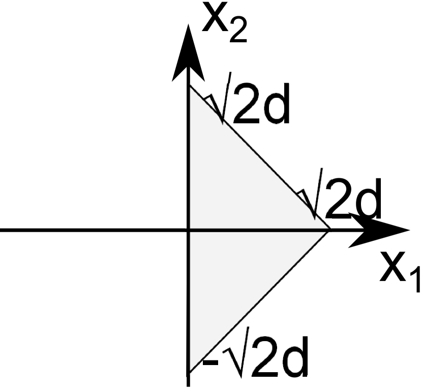
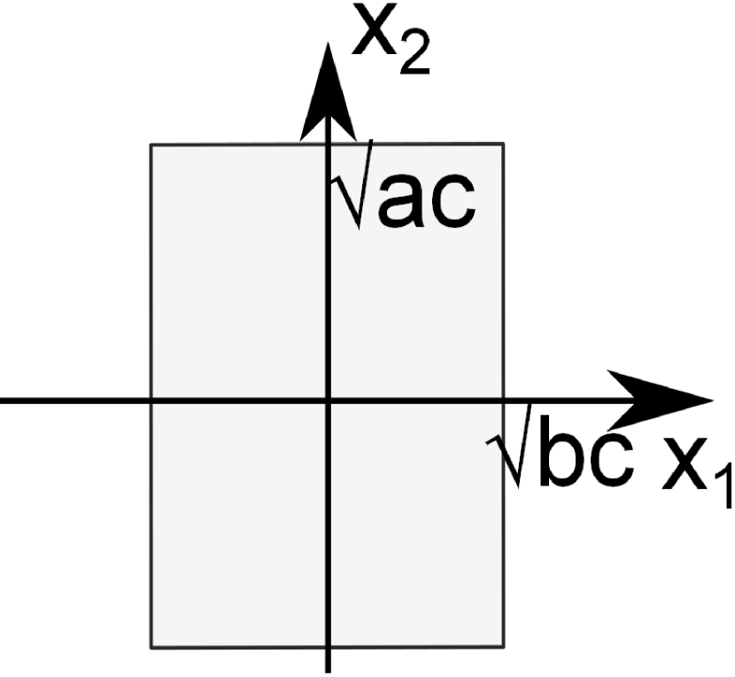
Fig. 3: The domains of $x_{1},x_{2}$.

If we rotate the square box on $45^{\circ}$ we will get the rhombus with the side $d$. As the solution of the Schrödinger equation (12) for such system we can take the following function

$$\widetilde{\Phi}(x_{1},x_{2}) = B\sin(n_{1}(x_{1}+x_{2}))\sin(n_{2}(x_{1}-x_{2})),$$ (14)

where $B$ is a normalization parameter. The boundary conditions are

$$\widetilde{\Phi}(x_{1},x_{2}=\pm x_{1}+\sqrt{2}d)=\widetilde{\Phi}(x_{1},x_{2}=\pm x_{1}-\sqrt{2}d)=0.$$

Hence, the parameters of the solution (14) are $n_{1}=\frac{\pi N_{1}}{\sqrt{2}d}$, $n_{2}=\frac{\pi N_{2}}{\sqrt{2}d}$, $N_{1},N_{2}=0,\pm 1,\pm 2,\ldots$.

Moreover, dividing the rhombus domain at zero boundary, we get the triangle box. The latter case is called the quantum triangle billiard. As the initial step we study the billiard where the sides of the triangle are obtained by the intersections of the three lines described by the following equations

$$x_{1}=0,\quad x_{2}=x_{1}-\sqrt{2}d,\quad x_{2}=-x_{1}+\sqrt{2}d$$ (15)

Hence, the boundary conditions for such system are

$$f(x_{1}=0,x_{2})=f(x_{1},x_{2}=\pm x_{1}+\sqrt{2}d) = f(x_{1},x_{2}=\pm x_{1}-\sqrt{2}d)=0.$$

One should note here that all the latter conditions must be fulfilled simultaneously, which means that the solutions are equal to zero on the sides of the triangle given by (15). As the solution of the Schrödinger equation (12) that satisfy the latter conditions let us select the following function

$$f(x_{1},x_{2}) = K(\widetilde{\Phi}(x_{1},x_{2})-\widetilde{\Phi}(-x_{1},x_{2})),$$ (16)

where $K$ is a normalization parameter. The other parameters of the solution (16) are $n_{1}=\frac{\pi N_{1}}{\sqrt{2}d}$, $n_{2}=\frac{\pi N_{2}}{\sqrt{2}d}$, $N_{1},N_{2}=0,\pm 1,\pm 2,\ldots$.

Finnaly, let us introduce the boundary conditions for the rectangle box. To this end we first study the square box with the side $d$ and the Schrödinger equation of the following form

$$-\left(\frac{1}{2a}\frac{\partial^{2}}{\partial x_{1}^{2}}+\frac{1}{2b}\frac{\partial^{2}}{\partial x_{2}^{2}}\right)\Phi(x_{1},x_{2})=E\Phi(x_{1},x_{2})$$ (17)

with the parameters of the Hamiltonian $a$ and $b$. The energy is $E_{N_{1},N_{2}}=\frac{1}{2}\left(\frac{n_{1}^{2}}{a}+\frac{n_{2}^{2}}{b}\right)$, $n_{1}=\frac{\pi N_{1}}{d}$, $n_{2}=\frac{\pi N_{2}}{d}$, $N_{1},N_{2}=0,\pm 1,\pm 2,\ldots$ and the solution of the latter equation is given by (13). Let us make the transformation to the new variables $y_{1}=\sqrt{a}x_{1}$, $y_{2}=\sqrt{b}x_{2}$. The transformed Schrödinger equation (17) is the folowing

$$-\frac{1}{2}\left(\frac{\partial^{2}}{\partial y_{1}^{2}}+\frac{\partial^{2}}{\partial y_{2}^{2}}\right)\Phi\left(\frac{y_{1}}{\sqrt{a}},\frac{y_{2}}{\sqrt{b}}\right)=E\Phi\left(\frac{y_{1}}{\sqrt{a}},\frac{y_{2}}{\sqrt{b}}\right),$$

where the solution can be written as

$$\Phi\left(\frac{y_{1}}{\sqrt{a}},\frac{y_{2}}{\sqrt{b}}\right) = A\sin\left(n_{1}\frac{y_{1}}{\sqrt{a}}\right)\sin\left(n_{2}\frac{y_{2}}{\sqrt{b}}\right)$$

Thus, the boundary conditions for the rectangle domain with the sides $d\sqrt{a}$, $d\sqrt{b}$ are

$$\Phi\left(y_{1}=\pm d\sqrt{a},\frac{y_{2}}{\sqrt{b}}\right) = \Phi\left(\frac{y_{1}}{\sqrt{a}},y_{2}=\pm d\sqrt{b}\right)=0.$$

We can conclude, that one can obtained the boundary conditions for the specific forms of boxes using the knowledge about the boundary conditions of the well known squar box case.

4. Time evolution of the center-of-mass covariance

Since the center of mass coordinates are dependent we are interested in there covariance time evolution for the bounded and unbounded problems. By definition, the square modulus of the wave function is the probability density function

$$f(X_{c},x,t) = \Big{|}\Phi(X_{c},x,t)\Big{|}^{2}.$$

Thus, the expectations for $X_{c}$, $x$ and $X_{c}\cdot x$ are the following

$$\mathbb{E}(x) = \int\limits_{-\infty}^{\infty}d\widetilde{x}\int\limits_{-\infty}^{\infty}\widetilde{X}f(\widetilde{X},x,t)d\widetilde{X},\quad\mathbb{E}(X_{c})=\int\limits_{-\infty}^{\infty}d\widetilde{x}\int\limits_{-\infty}^{\infty}\widetilde{x}f(X_{c},\widetilde{x},t)d\widetilde{X},$$

$$\mathbb{E}(X_{c}\cdot x) = \int\limits_{-\infty}^{\infty}d\widetilde{x}\int\limits_{-\infty}^{\infty}\widetilde{X}\widetilde{x}f(\widetilde{X},\widetilde{x},t)d\widetilde{X}$$

and the covariance of $X_{c}$ and $x$ is

$$Cov(X_{c},x,t) = \mathbb{E}(X_{c}\cdot x)-\mathbb{E}(X_{c})\mathbb{E}(x)=\langle\Phi(X_{c},x,t)|X_{c}x|\Phi(X_{c},x,t)\rangle$$

$$- \langle\Phi(X_{c},x,t)|X_{c}|\Phi(X_{c},x,t)\rangle\langle\Phi(X_{c},x,t)|x|\Phi(X_{c},x,t)\rangle.$$

However, we can just substitute the definition of $X_{c}$ and $x$ in (4.) and get the equivalent result

$$Cov(X_{c},x,t) = \mathbb{E}((\mu_{1}x_{1}+\mu_{2}x_{2})(x_{1}-x_{2}))-\mathbb{E}(\mu_{1}x_{1}+\mu_{2}x_{2})\mathbb{E}(x_{1}-x_{2})$$

$$= \mu_{1}\left(\mathbb{E}(x_{1}^{2})-\mathbb{E}^{2}(x_{1})\right)-\mu_{2}\left(\mathbb{E}(x_{2}^{2})-\mathbb{E}^{2}(x_{2})\right)$$

$$= \mu_{1}\left(\langle\Phi(x_{1},x_{2},t)|x_{1}^{2}|\Phi(x_{1},x_{2},t)\rangle-\left(\langle\Phi(x_{1},x_{2},t)|x_{1}|\Phi(x_{1},x_{2},t)\rangle\right)^{2}\right)$$

$$- \mu_{2}\left(\langle\Phi(x_{1},x_{2},t)|x_{2}^{2}|\Phi(x_{1},x_{2},t)\rangle-\left(\langle\Phi(x_{1},x_{2},t)|x_{2}|\Phi(X_{c},x,t)\rangle\right)^{2}\right).$$

In the case of the equal masses the covariance is zero. Note that we must change the variables in the state function before integrating (4.).

4.1. Examples

To obtain the covariance, one need to select some time state $\Phi(X_{c},x,t)$ ($\Phi(X_{c},x,t)$). Using the evolution operator we can obtain any state $|\Phi(t)\rangle$ from the initial one $|\Phi(0)\rangle$ as

$$|\Phi(X_{c},x,t)\rangle=e^{-\frac{iHt}{\hbar}}|\Phi(X_{c},x,0)\rangle.$$

The evolution operator can be written as

$$e^{-\frac{iHt}{\hbar}} = e^{-\frac{i}{\hbar}\frac{P^{2}}{2M}t}e^{-\frac{i}{\hbar}\frac{p^{2}}{2\mu}t}.$$

If the problem is unbounded the well known Baker-Hausdorff formula [33] can be used $e^{\xi\widehat{A}}\widehat{B}e^{-\xi\widehat{A}}=\widehat{B}+\xi[\widehat{A}\widehat{B}]+\frac{\xi^{2}}{2}[\widehat{A}[\widehat{A}\widehat{B}]]+\ldots$ and

$$e^{\frac{iHt}{\hbar}}X_{c}xe^{-\frac{iHt}{\hbar}}=\left(e^{\frac{i}{\hbar}\frac{P^{2}}{2M}t}X_{c}e^{-\frac{i}{\hbar}\frac{P^{2}}{2M}t}\right)\left(e^{\frac{i}{\hbar}\frac{p^{2}}{2\mu}t}xe^{-\frac{i}{\hbar}\frac{p^{2}}{2\mu}t}\right)=\left(X_{c}+\frac{P}{M}t\right)\left(x+\frac{p}{\mu}t\right)$$ (20)

holds. Hence, the expectations are

$$\langle\Phi(t)|X_{c}x|\Phi(t)\rangle = \langle\Phi(0)|e^{\frac{iHt}{\hbar}}X_{c}xe^{-\frac{iHt}{\hbar}}|\Phi(0)\rangle=\langle\Phi(0)|\left(X_{c}+\frac{P}{M}t\right)\left(x+\frac{p}{\mu}t\right)|\Phi(0)\rangle,$$

$$\langle\Phi(t)|X_{c}|\Phi(t)\rangle = \langle\Phi(0)|e^{\frac{iHt}{\hbar}}X_{c}e^{-\frac{iHt}{\hbar}}|\Phi(0)\rangle=\langle\Phi(0)|\left(X_{c}+\frac{P}{M}t\right)|\Phi(0)\rangle,$$

$$\langle\Phi(t)|x|\Phi(t)\rangle = \langle\Phi(0)|e^{\frac{iHt}{\hbar}}xe^{-\frac{iHt}{\hbar}}|\Phi(0)\rangle=\langle\Phi(0)|\left(x+\frac{p}{\mu}t\right)|\Phi(0)\rangle$$

and the covariance of $X_{c}$ and $x$ for the unbounded problem evolve in time as

$$Cov(X_{c},x,t) = \langle\Phi(0)|\left(X_{c}+\frac{P}{M}t\right)\left(x+\frac{p}{\mu}t\right)|\Phi(0)\rangle$$

$$- \langle\Phi(0)|\left(X_{c}+\frac{P}{M}t\right)|\Phi(0)\rangle\langle\Phi(0)|\left(x+\frac{p}{\mu}t\right)|\Phi(0)\rangle.$$

For the bounded problem we can not use the Baker-Hausdorff formula since the variables $X_{c}$ and $x$ are dependent. As an example, let us take as the state $\Phi(X_{c},x,t)$ the function that depends only from $\{n_{1},n_{2}\}=\{(1,1),(2,2)\}$ and has the following view

$$\Phi(X_{c},x,t) = A_{1}\widetilde{\Psi}_{11}(X_{c},x)e^{-iE_{11}t/\hbar}+A_{2}\widetilde{\Psi}_{22}(X_{c},x)e^{-iE_{22}t/\hbar}.$$

Hence, the probability density function is

$$f(X_{c},x,t) = A_{1}^{2}\widetilde{\Psi}^{2}_{11}(X_{c},x)+A_{2}^{2}\widetilde{\Psi}^{2}_{22}(X_{c},x)$$

$$\cdot +2A_{1}A_{2}\widetilde{\Psi}_{11}(X_{c},x)\widetilde{\Psi}_{22}(X_{c},x)\cos\left((E_{11}-E_{22})t/\hbar\right).$$

From the normalization condition we can choose $A_{1}=A_{2}=\frac{2}{d}$. Since for the bounded problem the coordinates $X_{c}$ and $x$ are in the domain shown in Fig. 1, the covariance (4.) is the following

$$Cov(X_{c},x,t) = -\frac{d^{2}(m_{1}-m_{2})}{165888\pi^{4}M}\Bigg{(}(668288-61440\pi^{2})\cos\left((E_{11}-E_{22})t/\hbar\right)$$

$$+ 102400\cos^{2}\left((E_{11}-E_{22})t/\hbar\right)+8640\pi^{2}-4608\pi^{4}+50625\Bigg{)},$$

where $E_{11}-E_{22}=\frac{-3\hbar^{2}\pi^{2}}{2d^{2}\mu}$, $\mu=m_{1}m_{2}/M$. Certainly, the latter example is given for the illustrative purposes. To get the more general covariance we need to find the state $|\Phi(t)\rangle$ for the bounded problem. To this end, the Green’s function theory can be applied.

5. Green’s function and time evolution

In [37] the propagator is investigated for the case of the one particle confined in the box. The relation between the wave function at time $t$ and $0$ is given by the following formula

$$\Psi(X_{c},x,t)=i\hbar\int\limits_{-\infty}^{\infty}\Psi(x_{1},x_{2})G(X_{c},x,x_{1},x_{2},t)dx_{1}dx_{2},$$

where $G(X_{c},x,x_{1},x_{2},t)$ is a time dependent Green’s function or the propagator. In [35] the Green’s function is represented in terms of theta-three function

$$G(\xi,\eta,\tau) = \frac{1}{2d}(\theta_{3}(\xi,\tau)-\theta_{3}(\eta,\tau)),$$

where the theta-three function is

$$\theta_{3}(\zeta,\tau) = \sum\limits_{n=-\infty}^{\infty}e^{2in\zeta}e^{i\pi n^{2}\tau}.$$

In the Whittaker and Watsou notation [36] it can be represented as

$$\theta_{3}(\zeta,q) = 1+2\sum\limits_{n=1}^{\infty}\cos(2n\zeta)q^{n^{2}},\quad q=e^{i\pi\tau}.$$ (22)

Hence, the propagator for the one particle is

$$G(x,x^{\prime},t) = \frac{1}{2d}\sum\limits_{n=-\infty}^{\infty}e^{2in(x-x^{\prime})}e^{i\pi n^{2}t}.$$

It is obvious, that the propagator for the two particles can be written as

$$G(X_{c},x,x_{1},x_{2},t)=\frac{1}{4d^{2}}(\theta_{3}(X_{c},t)-\theta_{3}(x_{1},t))(\theta_{3}(x,t)-\theta_{3}(x_{2},t))$$

$$= \frac{1}{4d^{2}}\left(\sum\limits_{n=-\infty}^{\infty}e^{2inX_{c}}e^{i\pi n^{2}t}-\sum\limits_{n=-\infty}^{\infty}e^{2inx_{1}}e^{i\pi n^{2}t}\right)$$

$$\cdot \left(\sum\limits_{k=-\infty}^{\infty}e^{2ikx}e^{i\pi k^{2}t}-\sum\limits_{k=-\infty}^{\infty}e^{2ikx_{2}}e^{i\pi k^{2}t}\right).$$

As the initial state $\Psi(x_{1},x_{2},0)$ one can select the following function

$$\Phi(x_{1},x_{2},0) = \pm\frac{1}{\sqrt{2}d}\left(\sin\left(\frac{\pi}{d}x_{1}\right)\sin\left(\frac{\pi}{d}x_{2}\right)+\sin\left(\frac{2\pi}{d}x_{1}\right)\sin\left(\frac{2\pi}{d}x_{2}\right)\right).$$

Thus, we can write

$$\Psi(X_{c},x,t)=\frac{i\hbar}{4d^{2}}\Bigg{(}\theta_{3}(X_{c},t)\theta_{3}(x,t)\int\limits_{0}^{d}\int\limits_{0}^{d}\Psi(x_{1},x_{2},0)dx_{1}dx_{2}$$

$$- \theta_{3}(x,t)\int\limits_{0}^{d}\int\limits_{0}^{d}\Psi(x_{1},x_{2},0)\theta_{3}(x_{1},t)dx_{1}dx_{2}$$

$$\cdot -\theta_{3}(X_{c},t)\int\limits_{0}^{d}\int\limits_{0}^{d}\Psi(x_{1},x_{2},0)\theta_{3}(x_{2},t)dx_{1}dx_{2}$$

$$+ \int\limits_{0}^{d}\int\limits_{0}^{d}\Psi(x_{1},x_{2},0)\theta_{3}(x_{1},t)\theta_{3}(x_{2},t)dx_{1}dx_{2}\Bigg{)}$$

$$= \frac{i\hbar\sqrt{2}}{4d}\Bigg{(}\theta_{3}(X_{c},t)\theta_{3}(x,t)\frac{2}{\pi^{2}}-(\theta_{3}(X_{c},t)+\theta_{3}(x,t))\sum\limits_{n=-\infty}^{\infty}\frac{1+e^{2idn}}{\pi^{2}-4d^{2}n^{2}}e^{i\pi n^{2}t}$$

$$+ \frac{\pi^{2}}{2}\left(\sum\limits_{n=-\infty}^{\infty}\frac{e^{2idn}+1}{\pi^{2}-4d^{2}n^{2}}e^{i\pi n^{2}t}\right)^{2}+\frac{\pi^{2}}{8}\left(\sum\limits_{n=-\infty}^{\infty}\frac{e^{2idn}-1}{\pi^{2}-d^{2}n^{2}}e^{i\pi n^{2}t}\right)^{2}\Bigg{)}.$$

Using that

$$\frac{1}{ix}=\int_{0}^{\infty}\exp\left(-izx\right)dz$$

we can write

$$\frac{1}{i(\pi^{2}-4d^{2}n^{2})}=\int_{0}^{\infty}\exp\left(-iz(\pi^{2}-4d^{2}n^{2})\right)dz.$$

Substituting $\Psi(X_{c},x,t)$ in (4.) the covariance time evolution can be obtained.

5.1. The Green’s function and the special boundary shapes

Let us find the Green’s function for the four boundary shapes presented in Sec. 3. By definition the Green’s function is the following

$$G(x_{1},x_{2},x_{1}^{\prime},x_{2}^{\prime},t)=\sum\limits_{N_{1}=-\infty}^{\infty}\sum\limits_{N_{2}=-\infty}^{\infty}\Phi_{N_{1},N_{2}}(x_{1},x_{2},t)\Phi^{\ast}_{N_{1},N_{2}}(x_{1}^{\prime},x_{2}^{\prime})\exp(-iE_{N_{1},N_{2}}t).$$ (23)

For the square box domain the energy is $E_{N_{1},N_{2}}=\frac{n_{1}^{2}+n_{2}^{2}}{2m}=\frac{\pi^{2}(N_{1}^{2}+N_{2}^{2})}{2md^{2}}$, $n_{1}=\frac{\pi N_{1}}{d}$, $n_{2}=\frac{\pi N_{2}}{d}$, $N_{1},N_{2}=0,\pm 1,\pm 2,\ldots$. Hence, for the latter boundary shape the Green’s function (23) is the following

$$G(x_{1},x_{2},x_{1}^{\prime},x_{2}^{\prime},t)=A^{2}\sum\limits_{N_{1},N_{2}=-\infty}^{\infty}\sin(n_{1}x_{1})\sin(n_{2}x_{2})\sin(n_{1}x_{1}^{\prime})\sin(n_{2}x_{2}^{\prime})e^{-iE_{N_{1}N_{2}t}}$$

$$= \frac{A^{2}}{4}\sum\limits_{N_{1}=-\infty}^{\infty}\left(\cos\left(\frac{\pi N_{1}}{d}(x_{1}+x_{1}^{\prime})\right)-\cos\left(\frac{\pi N_{1}}{d}(x_{1}-x_{1}^{\prime})\right)\right)e^{-\frac{i\pi^{2}N_{1}^{2}}{2md^{2}}t}$$

$$\cdot \sum\limits_{N_{2}=-\infty}^{\infty}\left(\cos\left(\frac{\pi N_{2}}{d}(x_{2}+x_{2}^{\prime})\right)-\cos\left(\frac{\pi N_{2}}{d}(x_{2}-x_{2}^{\prime})\right)\right)e^{-\frac{i\pi^{2}N_{2}^{2}}{2md^{2}}t}$$

where we used the known formula $\sin\alpha\sin\beta=\frac{1}{2}\left(\cos(\alpha-\beta)-\cos(\alpha+\beta)\right)$. Using the following notations

$$\eta_{1}=\frac{\pi}{2d}(x_{1}-x_{1}^{\prime}),\quad\eta_{2}=\frac{\pi}{2d}(x_{1}+x_{1}^{\prime}),\quad\eta_{3}=\frac{\pi}{2d}(x_{2}-x_{2}^{\prime}),$$

$$\eta_{4}=\frac{\pi}{2d}(x_{2}+x_{2}^{\prime}),\quad\tau=\frac{-\pi t}{2md^{2}}.$$

we can rewrite the latter Green’s function in a short form

$$G(\eta_{1},\eta_{2},\eta_{3},\eta_{4},\tau) = \frac{A^{2}}{4}\sum\limits_{N_{1}=-\infty}^{\infty}\left(\cos(2\eta_{1}N_{1})-\cos(2\eta_{2}N_{1})\right)e^{i\pi\tau N_{1}^{2}}$$

$$\cdot \sum\limits_{N_{2}=-\infty}^{\infty}\left(\cos(2\eta_{3}N_{2})-\cos(2\eta_{4}N_{2})\right)e^{i\pi\tau N_{2}^{2}}.$$

Since $N_{1}=0,\pm 1,\pm 2,\ldots$ we can split the latter sums into two sums as

$$G(\eta_{1},\eta_{2},\eta_{3},\eta_{4},\tau) = \frac{A^{2}}{4}\Bigg{(}\sum\limits_{N_{1}=1,2,\ldots}^{\infty}\left(\cos(2\eta_{1}N_{1})-\cos(2\eta_{2}N_{1})\right)e^{i\pi\tau N_{1}^{2}}$$

$$+ \sum\limits_{N_{1}=-1,-2,\ldots}^{-\infty}\left(\cos(2\eta_{1}N_{1})-\cos(2\eta_{2}N_{1})\right)e^{i\pi\tau N_{1}^{2}}\Bigg{)}$$

$$\cdot \Bigg{(}\sum\limits_{N_{2}=1,2,\ldots}^{\infty}\left(\cos(2\eta_{3}N_{2})-\cos(2\eta_{4}N_{2})\right)e^{i\pi\tau N_{2}^{2}}$$

$$+ \sum\limits_{N_{2}=-1,-2,\ldots}^{\infty}\left(\cos(2\eta_{3}N_{2})-\cos(2\eta_{4}N_{2})\right)e^{i\pi\tau N_{2}^{2}}\Bigg{)}.$$

Using the definition of the theta three function (22) and the notation $q=\exp(i\pi\tau)$ we can finally write that the Green’s function for the square box with the side $d$ is

$$G(\eta_{1},\eta_{2},\eta_{3},\eta_{4},q) = \frac{A^{2}}{4}\left(\theta_{3}(\eta_{1},q)-\theta_{3}(\eta_{2},q)\right)\left(\theta_{3}(\eta_{3},q)-\theta_{3}(\eta_{4},q)\right).$$

For the rhombus box we can use the similar technics as in the previous case. The energy is $E_{N_{1},N_{2}}=\frac{n_{1}^{2}+n_{2}^{2}}{m}=\frac{\pi^{2}(N_{1}^{2}+N_{2}^{2})}{2md^{2}}$, $n_{1}=\frac{\pi N_{1}}{\sqrt{2}d}$, $n_{2}=\frac{\pi N_{2}}{\sqrt{2}d}$, $N_{1},N_{2}=0,\pm 1,\pm 2,\ldots$ and the Green’s function for the rhombus with the side $d$ is the following

$$G_{r}(\eta_{1},\eta_{2},\eta_{3},\eta_{4},q) = B^{2}\left(\theta_{3}(\zeta_{1},q)-\theta_{3}(\zeta_{2},q)\right)\left(\theta_{3}(\zeta_{3},q)-\theta_{3}(\zeta_{4},q)\right),$$

where we used the notations

$$\zeta_{1}=\frac{\pi}{2\sqrt{2}d}(x_{1}-x_{2}-x_{1}^{\prime}-x_{2}^{\prime}),\quad\zeta_{2}=\frac{\pi}{2\sqrt{2}d}(x_{1}+x_{2}+x_{1}^{\prime}+x_{2}^{\prime}),\quad\tau=\frac{-\pi t}{2md^{2}}$$

$$\zeta_{3}=\frac{\pi}{2\sqrt{2}d}(x_{1}-x_{2}-x_{1}^{\prime}+x_{2}^{\prime}),\quad\zeta_{4}=\frac{\pi}{2\sqrt{2}d}(x_{1}-x_{2}+x_{1}^{\prime}-x_{2}^{\prime}),\quad q=e^{i\pi\tau}.$$

For the triangle billiard the energy is equal to $E_{N_{1},N_{2}}=2\frac{n_{1}^{2}+n_{2}^{2}}{m}=\frac{\pi^{2}(N_{1}^{2}+N_{2}^{2})}{md^{2}}$, $n_{1}=\frac{\pi N_{1}}{\sqrt{2}d}$, $n_{2}=\frac{\pi N_{2}}{\sqrt{2}d}$, $N_{1},N_{2}=0,\pm 1,\pm 2,\ldots$, $q=\exp(2i\pi\tau)$ and the corresponding Green’s function

$$G_{b}(\eta_{1},\eta_{2},\eta_{3},\eta_{4},q) = K^{2}\Bigg{(}\left(\theta_{3}(\zeta_{1},q)-\theta_{3}(\zeta_{2},q)\right)\left(\theta_{3}(\zeta_{3},q)-\theta_{3}(\zeta_{4},q)\right)$$

$$- \left(\theta_{3}(-\zeta_{1},q)-\theta_{3}(-\zeta_{2},q)\right)\left(\theta_{3}(-\zeta_{3},q)-\theta_{3}(-\zeta_{4},q)\right)\Bigg{)}$$

holds.

Finally, it is easy to verify, that for the rectangle domain the Green’s function is

$$G_{b}(\xi_{1},\xi_{2},\xi_{3},\xi_{4},q_{a},q_{b}) = A^{2}\left(\theta_{3}(\xi_{1},q_{a})-\theta_{3}(\xi_{2},q_{a})\right)\left(\theta_{3}(\xi_{3},q_{b})-\theta_{3}(\xi_{4},q_{b})\right),$$

where the following notations were introduced

$$\xi_{1}=\frac{\pi}{2\sqrt{a}d}(y_{1}-y_{1}^{\prime}),\quad\xi_{2}=\frac{\pi}{2\sqrt{a}d}(y_{1}+y_{1}^{\prime}),\quad\tau_{a}=\frac{-\pi t}{2ad^{2}},\quad\tau_{b}=\frac{-\pi t}{2bd^{2}}$$

$$\xi_{3}=\frac{\pi}{2\sqrt{a}d}(y_{2}-y_{2}^{\prime}),\quad\xi_{4}=\frac{\pi}{2\sqrt{a}d}(y_{2}+y_{2}^{\prime}),\quad q_{a}=e^{i\pi\tau_{a}},\quad q_{b}=e^{i\pi\tau_{b}}.$$

5.1.1. Example

As an example let us check the obtained Green’s function corresponding to the square impenetrable box with the side $d$. If the initial state is (13) one can write

$$\Psi(x_{1},x_{2},t) = \int\limits_{-d}^{d}\int\limits_{-d}^{d}A\sin(n_{1}y_{1})\sin(n_{2}y_{2})\frac{A^{2}}{4}\left(\theta_{3}(\frac{\pi}{2d}(x_{1}-y_{1}),q)-\theta_{3}(\frac{\pi}{2d}(x_{1}+y_{1}),q)\right)$$ (24)

$$\cdot \left(\theta_{3}(\frac{\pi}{2d}(x_{2}-y_{2}),q)-\theta_{3}(\frac{\pi}{2d}(x_{2}+y_{2}),q)\right)dy_{1}dy_{2}$$

$$= \frac{A^{3}}{4}\int\limits_{-d}^{d}\sin(n_{1}y_{1})\sum\limits_{N_{1}=1}^{\infty}q^{N_{1}^{2}}(\cos(\frac{N_{1}\pi}{d}(x_{1}-y_{1}))-\cos(\frac{N_{1}\pi}{d}(x_{1}+y_{1})))dy_{1}$$

$$\cdot \int\limits_{-d}^{d}\sin(n_{2}y_{2})\sum\limits_{N_{2}=1}^{\infty}q^{N_{2}^{2}}(\cos(\frac{N_{1}\pi}{d}(x_{2}-y_{2}))-\cos(\frac{N_{1}\pi}{d}(x_{2}+y_{2})))dy_{2}$$

The integrals are the following

$$\int\limits_{-d}^{d}\sin\left(\frac{\pi N_{1}}{d}y_{1}\right)(\cos(\frac{N_{1}\pi}{d}(x_{1}-y_{1}))-\cos(\frac{N_{1}\pi}{d}(x_{1}+y_{1})))dy_{1}$$

$$= \frac{d}{\pi N_{1}}(2\pi N_{1}-\sin(2\pi N_{1}))\sin\left(\frac{\pi N_{1}}{d}x_{1}\right).$$

Hence, substituting the latter result in (24) we can write

$$\Psi(x_{1},x_{2},t) = A^{3}d^{2}\sum\limits_{N_{1},N_{2}=1}^{\infty}q^{N_{1}^{2}+N_{2}^{2}}\sin\left(\frac{\pi N_{1}}{d}x_{1}\right)\sin\left(\frac{\pi N_{2}}{d}x_{2}\right).$$

Since $A=1/d$ we get the known state

$$\Psi(x_{1},x_{2},t)=A\sum\limits_{N_{1},N_{2}=1}^{\infty}e^{-\frac{i\pi^{2}t}{2md^{2}}(N_{1}^{2}+N_{2}^{2})}\sin\left(\frac{\pi N_{1}}{d}x_{1}\right)\sin\left(\frac{\pi N_{2}}{d}x_{2}\right).$$

Hence, the obtained Green’s function is correct.

6. Summary

In this last section we wish to summarize and point out the main results reached in this paper. Our first conclusion is that the separability of the Schrödinger equation of an unconstrained system of two particles, coupled or not, generally brakes when boundary condition of geometric nature (holonomic constrains) are taken into consideration. The main reason of such behavior may be traced back to the ”coupling” get established between the ”coordinates” as a consequence of the algebraic equations describing the same constraints. We have illustrated these point writing the Schrödinger equation of two noninteracting particles referred to $X_{c}$ and $x$, center of mass and relative motion coordinate, respectively. By imposing generalized confinement conditions on the system, that is limiting the region of motion and assuming impenetrability conditions, one is lead to equations relating $X_{c}$ and $x$ which makes, impossible the separation of $X_{c}$ and $x$ in the problem. It is remarkable that searching the stationary state of this constrained system exhibits the same mathematical formulation one should use to treat the problem of a single particle in a plane but confined in a domain whose shape depends on the boundary conditions imposed to the two-particle system. Moreover, free particle motion on the plane is studied. The domain of the motion restricted by the impenetrable walls forming the square, the rhombus, the triangle and the rectangle (billiards) are considered. The billiards are analyzed by studying the time evolution of the covariance of $X_{c}$ and $x$. To this end the Green’s function expressed in terms of the Jacobi $\theta_{3}$ function is applied.

References

- [1] S. W. Doescherand, M. H. Rice: Am. J. Phys. 37, 1246 (1969).
- [2] D. N. Pinder: Am. J. Phys. 58, 54 (1989).
- [3] D. W. Schlitt, C . Stutz: Am. J. Phys 38, 70 (1970).
- [4] V. V. Dodonov, A.B. Klimov, D.E. Nikonov: J. Math. Phys. 34, 3391 (1993).
- [5] S. Di Martino, F. Anz’a, P. Facchi, A. Kossakowski, G. Marmo, A. Messina, B. Militello, S. Pascazio: J. Phys. A 46, 365301 (2013).
- [6] F. Anz , S. Di Martino, A. Messina, B. Militello: Dynamics of a particle confined in a two-dimensional dilating and deforming domain Physica Scripta 90(7), 074062 (2015).
- [7] V. V. Dodonov, A. B. Klimov, V. I. Manko: Generation of squeesed states in a resonator with a moving wall Phys. Lett.A, 149(4), 225–228 (1990).
- [8] S. V. Mousavi: EPL 99, 30002 (2012).
- [9] S. V. Mousavi, Physics Letters A 377, 1513 (2013).
- [10] G. Guniberti, J. Yi, M. Porto: Appl. Phys. Lett 81, 850 (2002).
- [11] G. Zhang, X. Jiang, E. Wang: Science 300, 472 (2003).
- [12] J. M. Garcia, G. Medeiros-Ribeiro, K. Schmidt, T. Ngo, J. L. Feng, A. Lorke, J. Kotthaus, P. M. Petroff: Appl. Phys. Lett 71, 2014 (1997).
- [13] A. Lorke, R. J. Luyken, A. O. Govorov, J. P. Kotthaus, J. M. Garcia, P. M. Petroff: Phys. Rev. Lett 84, 2223 (2000).
- [14] K. D. Sen, A. K. Roy: Spherically confined isotropic harmonic oscillator Phys. Lett.A 357, 112–119 (2006).
- [15] V. G. Gueorguiev, A. R. P. Rau, and J. P. Draayer: Confined One Dimensional Harmonic Oscillator as a Two-Mode System Am.J. of Phys. 74(5), 394 (2006).
- [16] P. Amore, F.M. Fernandez: Two particle harmonic oscillator in a one dimensional box Acta Polytechnica 50, 17 (2010).
- [17] D. Djajaputra, B.R. Cooper: Hydrogen atom in a spherical well: linear approximation Eu. J. of Phy. 21(3), 261 (2000).
- [18] N. Aquino, E. Casta o: The confined two-dimensional hydrogen atom in the linear variational approach, Revista Mexicana de Fesica, 51 (2005).
- [19] F. M. Fernandez: The confined hydrogen atom with a moving nucleus Eu. J. of Phys. 7 (2009).
- [20] A. S. Dehkharghani, A. G. Volosniev, N. T. Zinner: Impenetrable mass-imbalanced particles in one-dimensional harmonic traps J. of Phys. A. 8(49), 085301 (2016).
- [21] V. V. Dodonov, V. I. Man’ko: Invariants and the Evolution of Nonstationary Quantum Systems Proceedings of the P. N. Lebedev Physical Institute
- [22] I. A. Malkin, V. I. Manko: Coherent states and magnetic translations Phys. stat. solidi B 31(1), K15–K17 (1969).
- [23] M. Robnik: Classical dynamics of a family of billiards with analytic boundaries J. Phys. A Math. Gen. 16 (1983).
- [24] L. Bunimovich: On the ergodic properties of nowhere dispersing billiards Commun. Math. Phys. 65, 295–312 (1979).
- [25] Ya. G. Sinai: On the foundations of the ergodic hypothesis for a dynamical system of statistical mechanics Doklady Akademii Nauk SSSR (in Russian) 153 (6), 1261–1264. (in English, Sov. Math Dokl. 4 pp. 1818–1822) (1963).
- [26] E. J. Heller: Bound-State Eigenfunctions of Classically Chaotic Hamiltonian Systems: Scars of Periodic Orbits, Phys. Rev. Lett., 53, 1515–1518 (1984).
- [27] M. V. Berry, M. Wilkinson: Diabolical Points in the Spectra of Triangles Proc. R. Soc. Lond. A 392, 15–43 (1984).
- [28] R. Artuso, G. Casati, I. Guarneri: Numerical study on ergodic properties of triangular billiards Phys. Rev. E 55 (1997).
- [29] G. Casati, T. Prosen: Mixing Property of Triangular Billiards Phys. Rev. Lett. 83 (1999).
- [30] J. Aguirre, J.C. Vallejo, M. A. F. Sanjuán: Wada basins and chaotic invariant sets in the Hénon-Heiles system., Phys. Rev. E 64, (2001).
- [31] S. K. Joseph, M. A. F. Sanjuán: Entanglement Entropy in a Triangular Billiard, Entropy 18, 79 (2016).
- [32] C. Tanner: The role of boundary conditions in separation of variables: Quantum oscillator in a box Am. J. Phys. 59, 931–935 (1991).
- [33] W. Miller: Symmetry Groups and their Applications Academic Press, New York, 159–161 (1972).
- [34] Shen-xi Yu: Generalized center-of-mass coordinate and relative momentum operators studied through unitary transformations, Phys. Rev. A 54 (2) (1996).
- [35] T. Hannesson, S. M. Blinder: Theta-function representation for particle-in-a-box propagator Il Nuovo Cimento B Series 11 79 (2), 284–290 (1984).
- [36] E. T. Whittaker, G. N. Watson: A Course of Modern Analysis Cambridge University Press (1902).
- [37] S. A. Fulling, K. S. Güntürk: Exploring the propagator of a particle in a box Am. J. Phys. 71(55) (2003).
- [38] B. J. McCartin, Eigenstructure of the equilateral triangle, Part 1: The Dirichlet problem SIAM Review 45(2), 267–287 (2003).
- [39] F. Anzà, S. D. Martino, A. Messina, B. Militello: Dynamics of a particle confined in a two-dimensional dilating and deforming domain Physica Scripta 90(7), 074062 (2015). vol 183 (Moscow: Nauka), (1987) [tr. by Nova Science, New York, 1989.