Abstract

The apparent unification of gauge couplings in Grand Unified Theories around 10¹⁶ $\mathrm{Ge\kern-1.19995ptV}$ is one of the strong arguments in favor of Supersymmetric extensions of the Standard Model. In this paper, an analysis of the measurements of the strong coupling running from the CMS experiment at the LHC is combined with a “traditional” gauge coupling unification analysis using data at the Z peak. This approach places powerful constraints on the possible scales of new physics and on the parameters around the unification scale. A supersymmetric analysis without GUT threshold corrections describes the CMS data well and provides perfect unification. The favored scales are $M_{SUSY}\ =\ 2820\ +670\ -540\ \mathrm{Ge\kern-1.19995ptV}$ and $M_{GUT}\ =\ 1.05\pm 0.06\cdot 10^{16}\ \mathrm{Ge\kern-1.19995ptV}$. For zero or small threshold corrections the scale of new physics may be well within LHC reach.

1 Introduction

The Standard Model (SM) of particle physics works extremely well at collider energies. But it is incomplete, and the possible scale at which new physics phenomena could manifest themselves is a hot topic of great theoretical, experimental and practical interest.

When the LEP and SLC colliders came online, the weak coupling was measured with much higher precision, roughly on par with the precision for the electromagnetic coupling. In a renowned paper [1] from 1991 the famous plot was produced, showing that in contrast to the SM the Minimal Supersymmetric Standard Model (MSSM) leads to a single unification scale of a Grand Unified Theory (GUT), if we let the couplings run according to the MSSM theory:

$$M_{SUSY}=10^{3.0\pm 1.0}\mathrm{Ge\kern-1.19995ptV}\ ;\ M_{GUT}=10^{16.0\pm 0.3}\mathrm{Ge\kern-1.19995ptV}\ ;\ 1/\alpha_{GUT}=25.7\pm 1.7$$ (1)

where $M_{SUSY}$ is a single generic SUSY scale where the spectrum of supersymmetric (SUSY) particles starts to play a role by changing the running of the couplings, $M_{GUT}$ is the scale of grand unification where the electromagnetic, weak and strong coupling come together as an unified coupling $\alpha_{GUT}$.

In this paper indirect analyses based on the running of gauge couplings are performed to search for the scale of Supersymmetry, or any new physics that could change the running of the couplings. Two analyses are carried out:

• first a - by now “traditional”  - analysis of gauge coupling unification in a grand unification theory, using the latest experimental inputs at the Z peak scale, combined with a detailed statistical approach

• a novel analysis, including for the first time the measurements of the strong coupling by the CMS collaboration using the data collected at 7 $\mathrm{Te\kern-1.19995ptV}$ [3, 4, 5], which can shed light on the actual running of couplings from the Z peak to $\approx$ 1.4 $\mathrm{Te\kern-1.19995ptV}$.

2 Digression

If we are looking at the front of a train, we can see the lead locomotive but cannot tell much about the composition, or even how many locomotives are hauling it. If we are on the railway platform, we have a much better view.

In the first approach outlined above, in contrast to the SM the additional degree of freedom provided by the introduction of a new MSSM scale could lead to a single GUT unification scale, if we let the couplings run accordingly. It is amazing that we are trying to extrapolate from 10² to 10¹⁶ $\mathrm{Ge\kern-1.19995ptV}$. From experiments we know that even interpolation or modest extrapolations can be non-trivial. We measure the “offsets”, i.e. the values of the three couplings, around the Z peak and rely on theory to give us the “slopes” of the running couplings - without errors - up to the GUT scale. This may be an illusion e.g. new physics phenomena like extra dimensions could modify the running at intermediate scales, so the “unification” point may be imaginary.

In the second approach, we step on the railway platform. The actual running of the strong coupling provides a powerful constraint on new physics scenarios.

3 Definitions and Experimental Inputs

Throughout this paper the couplings are denoted as $\alpha_{i}$, $i\ =\ 1,2,3$. The values of $1/\alpha$ are used for plots and fit results. For the renormalization the modified minimal subtraction scheme ($\overline{MS}$) is used. The definitions are:

$$\alpha_{1}=\frac{5}{3}\frac{\alpha}{\mathrm{cos^{2}\theta_{\overline{MS}}}}$$ (2)

$$\alpha_{2}=\frac{\alpha}{\mathrm{sin^{2}\theta_{\overline{MS}}}}$$ (3)

$$\alpha_{3}=\frac{g_{s}^{2}}{4\pi}$$ (4)

where $\alpha$ is the electromagnetic coupling, $\mathrm{sin^{2}\theta_{\overline{MS}}}$ is the electroweak mixing angle in the $\overline{MS}$ scheme, and $\alpha_{3}$ is the strong coupling.

From Review of Particle Properties 2014 [2] (sections 10.2, 10.6, 9.3.12):

$$1/\alpha(M_{Z})=127.940\pm 0.014$$ (5)

$$\mathrm{sin^{2}\theta_{\overline{MS}}(M_{Z})}=0.23126\pm 0.00005$$ (6)

$$\alpha_{s}(M_{Z})=0.1185\pm 0.0006.$$ (7)

In 1991, at the Z mass scale $M_{Z}$, the relative errors in $\alpha(M_{Z})$, $\mathrm{sin^{2}\theta_{\overline{MS}}(M_{Z})}$ and $\alpha_{s}(M_{Z})$ were 0.24, 0.77 and 4.6 % respectively.

Now they are 0.011, 0.022 and 0.5 %, so we have improved enormously in the last quarter of a century. Even the measurements of the notoriously hard to extract strong coupling have gained an order of magnitude in precision. All this helps to improve the precision of the unification analyses.

In addition, for the second analysis, three measurements of the strong coupling by the CMS collaboration using the data collected at 7 $\mathrm{Te\kern-1.19995ptV}$ are utilized. They are using the ratio of the inclusive 3-jet cross section to the inclusive 2-jet cross section $R_{32}$ [3], inclusive jet cross sections up to 2 $\mathrm{Te\kern-1.19995ptV}$ in jet transverse momentum [4], and inclusive 3-jet production differential cross sections, where the invariant mass of the three jets is in the range of 445–3270 $\mathrm{Ge\kern-1.19995ptV}$ [5]. The Q values at which the strong coupling is measured are (474, 664, 896) $\mathrm{Ge\kern-1.19995ptV}$, (136, 226, 345, 521, 711, 1007) $\mathrm{Ge\kern-1.19995ptV}$ and (361, 429, 504, 602, 785, 1164, 1402) $\mathrm{Ge\kern-1.19995ptV}$ respectively. The 3-jet measurement reaches the highest scales.

4 Analysis Technique

A $\chi^{2}$ minimization with MINUIT for three parameters: $M_{SUSY}$, $M_{GUT}$ and $1/\alpha_{GUT}$ is used for the “traditional” analysis. The three couplings at $M_{Z}$ serve as input. The procedure is similar to the one used in [6, 7].

In the case of 1-loop Renormalization Group (RG) running of the couplings we can solve analytically; the coefficients for the 3 couplings are independent, given by the following SM or MSSM equation relating the couplings at scales $\mu$ and $\nu$:

$$1/\alpha_{i}(\nu)=1/\alpha_{i}(\mu)-(b_{i}/2\pi)\cdot ln(\nu/\mu).$$ (8)

In the SM above the top threshold the $b_{i}$ coefficients are (4.1, -3$\frac{1}{6}$, -7), while in the MSSM they have the values (6.6, 1, -3). As can be seen, the changes in slopes are substantial for all three couplings.

The high precision of the experimental inputs requires to use 2-loop RG running. In this case additional non-diagonal terms $b_{ij}$ (i,j = 1,2,3) appear in the equations, so the 3 couplings depend on each other and the error propagation is altered. The equations are solved numerically. Now the errors depend on the scale - for typical GUT scales they grow by 4, 12 and 6 % respectively for the three couplings.

The details of physics at the GUT scale are unknown. It may be necessary to apply a threshold correction to $\alpha_{3}(M_{GUT})$ in order to meet GUT boundary conditions. For detailed discussions of the nature, sign and size of these corrections we refer the reader to the reviews [8] and [2] (section 16.1.4) and references therein.

From a technical point of view, the threshold correction is applied as follows:

$$\alpha_{1}(M_{GUT})=\alpha_{2}(M_{GUT})=\alpha_{GUT}$$ (9)

$$\alpha_{3}(M_{GUT})=\alpha_{GUT}\cdot(1\ +\ \varepsilon_{GUT})$$ (10)

where $\varepsilon_{GUT}$ is the threshold correction for the strong coupling at the GUT scale. In practice, the higher precision of $1/\alpha_{1}$ and $1/\alpha_{2}$ brings the GUT scale very close to their cross-point. The $1/\alpha_{3}$ line may “hit” or “miss” the unification point, depending on the situation.

In the second analysis, the $\chi^{2}$ minimization with MINUIT uses the same three parameters and adds the 16 CMS measurements, bringing the experimental inputs to 19. In this case the fit has 16 degrees of freedom (dof).

5 “Traditional” Running Couplings Analysis

I update the analyses [6]  and [7], using the same fitting procedure applied on the new more precise experimental inputs.

The results of the fits are summarized in Table 1.

Table 1: Fit results - all for 2-loop RG running.

Threshold correction	$M_{SUSY}$	$M_{GUT}$	$1/\alpha_{GUT}$
[%]	[$\mathrm{Ge\kern-1.19995ptV}$]	[$\mathrm{Ge\kern-1.19995ptV}$]
$\pm$ 0	$10^{3.45\pm 0.09}$	$10^{16.02\pm 0.03}$	$25.83\pm 0.16$
- 3	$10^{2.03\pm 0.14}$	$10^{16.48\pm 0.04}$	$23.28\pm 0.26$
- 4	$10^{1.48\pm 0.11}$	$10^{16.66\pm 0.03}$	$22.28\pm 0.20$

The MSSM can still provide coupling unification at a GUT scale well below the Planck scale for the full set of precise 2014 measurements. But it is not without problems, which may be overlooked. As stated in [2] (section 16.1.4): “A small threshold correction at $M_{GUT}$ ($\varepsilon_{GUT}\sim-3\%\ \mathrm{to}\ -4\%$) is sufficient to fit the low energy data precisely.”  Actually threshold corrections of this size tend to push the SUSY scale to uncomfortably low regions, being progressively ruled out by the LHC experiments. For a threshold correction of -4% the fitted SUSY scale is $M_{SUSY}$  = 30 +9 -7 $\mathrm{Ge\kern-1.19995ptV}$, and for a threshold correction of -3% the SUSY scale goes up only to $M_{SUSY}$  = 107 +41 -30 $\mathrm{Ge\kern-1.19995ptV}$. In contrast a threshold correction of 0 % brings the SUSY scale to $\sim$ 3 $\mathrm{Te\kern-1.19995ptV}$.

6 Combined Analysis of CMS Data and Gauge Coupling Unification

In [7] a fit to the precise LEP2 $\mathrm{q\bar{q}}$ cross section measurements above the Z pole [9], with all three couplings running simultaneously, was pioneered. In addition, the effects of a low SUSY scale were compared to the then available measurements of the strong coupling running above the Z - from a LEP2 combination [12], and from the CDF experiment [13]. The analysis was limited by the top LEP2 energy or the relatively large uncertainties of the CDF result.

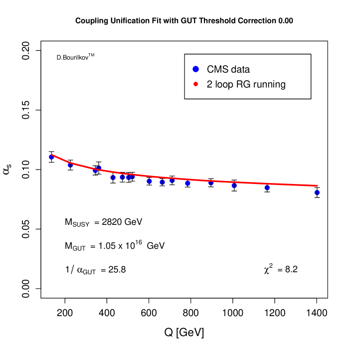
Figure 1: Top: Coupling unification fit of the CMS $\alpha_{s}$ measurements with GUT threshold correction of 0%. Bottom: The fitted running of the three couplings around the GUT scale. The fit describes well the CMS measurements and works well at the GUT scale.

Precision measurements of the strong coupling $\alpha_{s}$ well above the Z pole can provide a new window. This coupling changes the fastest in this energy range, but is also the hardest to measure. Recalling the metaphor from section 2, while the above mentioned analysis [7] just stepped at the end of the railway platform, the new CMS measurements of the running of the strong coupling in a vast area above the Z peak up to 1.4 $\mathrm{Te\kern-1.19995ptV}$ allow for a much more central view.

A fit to the data computing the running of the couplings from the Z peak to the highest LHC energies in the SM or in MSSM is performed. The results for different GUT threshold corrections are summarized in Table 2.

Table 2: Combined fit results - CMS data and GUT unification.

Threshold correction	$M_{SUSY}$	$M_{GUT}$	$1/\alpha_{GUT}$	$\chi^{2}$
[%]	[$\mathrm{Ge\kern-1.19995ptV}$]	[$\mathrm{Ge\kern-1.19995ptV}$]
+ 1	$10^{3.96\pm 0.10}$	$10^{15.85\pm 0.03}$	$26.74\pm 0.17$	8.2
$\pm$ 0	$10^{3.45\pm 0.09}$	$10^{16.02\pm 0.03}$	$25.83\pm 0.16$	8.2
- 1	$10^{3.02\pm 0.08}$	$10^{16.16\pm 0.03}$	$25.07\pm 0.15$	9.5
- 2	$10^{2.78\pm 0.07}$	$10^{16.25\pm 0.02}$	$24.63\pm 0.13$	25.1
- 3	$10^{2.60\pm 0.06}$	$10^{16.31\pm 0.02}$	$24.28\pm 0.10$	68.1
- 4	$10^{2.42\pm 0.05}$	$10^{16.38\pm 0.02}$	$23.95\pm 0.09$	138.3
- 5	$10^{2.26\pm 0.05}$	$10^{16.44\pm 0.02}$	$23.66\pm 0.09$	235.7

For a threshold correction of 0%, the 2-loop RG running provides an excellent fit for the CMS data and perfect unification, as shown in Figure 1. The favored SUSY scale is 2820 $\mathrm{Ge\kern-1.19995ptV}$, which means that the $\alpha_{s}$ measurements are well described by 2-loop SM running, as implemented in this analysis.

The $\chi^{2}/dof$ of the fit is $\sim 0.5$. This is not surprising, as the statistical and systematic errors are combined in quadrature. The correlations between the systematic errors are not provided and are not taken into account. They can be important both within each of the three CMS measurements, and on top of this hard to determine correlations between them could exist.

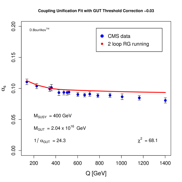
Figure 2: Top: Coupling unification fit of the CMS $\alpha_{s}$ measurements with GUT threshold correction of -3%. Bottom: The fitted running of the three couplings around the GUT scale. The fit fails on both counts as evidenced by the $\chi^{2}$: the CMS measurements are not well described and it does not work well at the GUT scale.

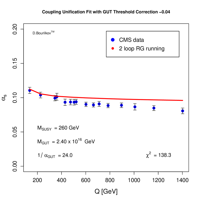
Figure 3: Top: Coupling unification fit of the CMS $\alpha_{s}$ measurements with GUT threshold correction of -4%. Bottom: The fitted running of the three couplings around the GUT scale. The fit fails on both counts as evidenced by the $\chi^{2}$: the CMS measurements are not well described and it does not work well at the GUT scale.

For a threshold correction of -3%, the fit runs into trouble on both ends. The unification point tries to push the SUSY scale down to low values (as in the “traditional” analysis), but this is not compatible with the CMS data. As a result the fit ends up with an unsatisfying compromise: a poor description of the CMS data and a “miss” at the GUT scale, as shown in Figure 2. The $\chi^{2}$ grows from 8.2 to 68.1. The situation is even more unsatisfactory for a threshold correction of -4%. Here the $\chi^{2}$ goes up to 138.7, see Figure 3.

A threshold correction of -1% is still fine. Here the $\chi^{2}$ goes up only to 9.5. The preferred SUSY scale in this case - 1050 $\mathrm{Ge\kern-1.19995ptV}$ - is high enough to be only weakly constrained by the CMS data. For a threshold correction of -2% the $\chi^{2}$ already reaches a value of 25.1.

In the opposite direction, a threshold correction of +1% (similar for higher corrections) is not impacted by the CMS data, as the SUSY scale is pushed up to 9120 $\mathrm{Ge\kern-1.19995ptV}$ while the GUT scale is pushed down to $0.7\cdot 10^{16}$. Positive threshold corrections may encounter different constraints. For example, baryon number is violated in GUT theories and in simple scenarios the proton lifetime is proportional to:

$$\tau_{p}\sim M_{GUT}^{4}\cdot(\frac{1}{\alpha_{GUT}})^{2}\cdot(\frac{1}{m_{p}})^{5}$$ (11)

The favored values for the GUT scale in this case will tend to push the proton lifetime lower, somewhat closer to the experimental limits $\sim$ 10³⁴ years [2] (section 16.1.5).

The quality of the GUT unification for different threshold corrections is visualized in Figure 4. Very small threshold corrections, consistent with zero (or within $\pm 1\%$) work very well and provide “perfect” unification. Negative corrections quickly diverge from a single unification point.

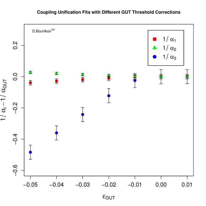
Figure 4: Quality of the coupling unification fits for different GUT threshold corrections $\varepsilon_{GUT}$. Clearly no or very small threshold corrections (within $\pm 1$ %) work best, while corrections of $\sim$ –3-4% fail to provide a single unification point.

It is interesting to note that the results without threshold corrections are very close to the values from the classical analysis [1], while the errors have improved by an order of magnitude. The best fit for the SUSY scale gives:

$$M_{SUSY}\ =\ 2820\ +670\ -540\ \mathrm{Ge\kern-1.19995ptV}.$$ (12)

The corresponding range from [1] was 100–10000 $\mathrm{Ge\kern-1.19995ptV}$. For a threshold correction of -1% the best fit is $M_{SUSY}\ =\ 1050\ +220\ -180\ \mathrm{Ge\kern-1.19995ptV}$.

In this paper a MSSM fit to the running couplings is used as a baseline. Similar analyses using the CMS measurements of the running of $\alpha_{s}$ can be performed for any new physics scenario affecting the couplings, if the relevant scales are in the measurement range. Many variations are possible. In [10] the CMS ratio of the inclusive 3-jet cross section to the inclusive 2-jet cross section (with highest point 896 $\mathrm{Ge\kern-1.19995ptV}$) is used to constrain simultaneously the $\alpha_{s}$ running and the scale (for different scenarios the limits range from 280–620 $\mathrm{Ge\kern-1.19995ptV}$). In [11] the CMS measurements [3, 5]s are used to constrain a scenario where direct detection of supersymmetric particles is impossible, but their existence can be manifested by precise measurements of the strong coupling running at $\mathrm{Te\kern-1.19995ptV}$ scales.

7 Outlook

In this paper, an analysis of the CMS measurements of the strong coupling running is combined with a “traditional” gauge coupling unification analysis. This approach places powerful constraints on the possible scales of new physics and on the parameters around the unification scale. An MSSM fit without GUT threshold corrections describes the CMS data well and provides perfect unification with scales:

$$M_{SUSY}\ =\ 2820\ +670\ -540\ \mathrm{Ge\kern-1.19995ptV}\ \ \ M_{GUT}\ =\ 1.05\pm 0.06\cdot 10^{16}\ \mathrm{Ge\kern-1.19995ptV}.$$

For zero or small threshold corrections the scale of new physics may be well within LHC reach.

So far the CMS collaboration has published only the measurements from the 7 $\mathrm{Te\kern-1.19995ptV}$ data. If the LHC experiments benefit fully from the increased energy and statistics in Run 2 to better control the systematics and to probe higher energy scales, they can extend substantially the reach for indirect evidence for the possible scale of new physics.

Acknowledgments

This work was started in the very productive environment of the University of Florida High Energy Physics group and completed during a stay at the LHC Physics Center of the Fermi National Accelerator Laboratory. The author wants to thank the LPC for the invitation to visit FNAL and for the kind hospitality.

References

- [1] U. Amaldi et al., Phys. Lett. B260 (1991) 447.
- [2] K.A. Olive et al. (Particle Data Group), Chin. Phys. C 38 (2014) 090001.
- [3] S. Chatrchyan et al. [CMS Collaboration], Eur. Phys. J. C 73 (2013) 10, 2604 [arXiv:1304.7498 [hep-ex]].
- [4] V. Khachatryan et al. [CMS Collaboration], Eur. Phys. J. C 75 (2015) 6, 288 [arXiv:1410.6765 [hep-ex]].
- [5] V. Khachatryan et al. [CMS Collaboration], Eur. Phys. J. C 75 (2015) 5, 186 [arXiv:1412.1633 [hep-ex]].
- [6] D. Bourilkov, Int. J. Mod. Phys. A 20 (2005) 3328 [hep-ph/0410350].
- [7] D. Bourilkov, AIP Conf. Proc. 842 (2006) 634 [hep-ph/0602168].
- [8] N. Polonsky, Lect. Notes Phys. M 68 (2001) 1 [hep-ph/0108236].
- [9] LEP Electroweak Working Group, Summer 2005 update, hep-ex/0511027.
- [10] D. Becciolini, M. Gillioz, M. Nardecchia, F. Sannino and M. Spannowsky, Phys. Rev. D 91 (2015) 1, 015010 [arXiv:1403.7411 [hep-ph]].
- [11] C. M. Ho and N. Okada, arXiv:1412.2734 [hep-ph].
-
[12]
LEP QCD Working Group (retrieved on August 17, 2015).
http://lepqcd.web.cern.ch/LEPQCD/annihilations/alphas_jun04/index.html. - [13] T. Affolder et al. [CDF Collaboration], Phys. Rev. Lett. 88 (2002) 042001 [hep-ex/0108034].