Nonparametric Bayesian Aggregation for Massive Data
Nonparametric Bayesian Aggregation for Massive Data
Abstract
We develop a set of scalable Bayesian inference procedures for a general class of nonparametric regression models. Specifically, nonparametric Bayesian inferences are separately performed on each subset randomly split from a massive dataset, and then the obtained local results are aggregated into global counterparts. This aggregation step is explicit without involving any additional computation cost. By a careful partition, we show that our aggregated inference results obtain an oracle rule in the sense that they are equivalent to those obtained directly from the entire data (which are computationally prohibitive). For example, an aggregated credible ball achieves desirable credibility level and also frequentist coverage while possessing the same radius as the oracle ball.
keywords:
[class=AMS] Primary 62C10 Secondary 62G15, 62G08keywords:
Credible region, divide-and-conquer, Gaussian process prior, linear functional, nonparametric Bayesian inference1 Introduction
With rapid development in modern technology, massive data sets are becoming more and more common. An important feature of massive data is their large volume which hinders applications of traditional statistical methods. For example, due to huge data amount and limited CPU memory, it is often impossible to process the entire data in a single machine. In the parallel computing environment, a common practice is to distribute massive data to multiple processors, and then aggregate local results in an efficient way. A series of frequentist methods such as [17, 24, 46, 47] have been proposed in this Divide-and-Conquer (D&C) framework.
In Bayesian community, there are quite a few computational or methodological works developed for massive data such as scalable algorithms for Bayesian variable selection ([36, 45]) and scalable posterior sampling in parametric models ([43, 44]). Theoretical guarantees of D&C methods have been recently obtained in robust estimation ([25]), approximation of posterior distributions ([19]), posterior interval estimation ([22]), credible sets of signal in Gaussian white noise ([20, 21]). Rather, the present paper puts focus on uncertainty quantification of the model parameter in general nonparametric regression, primarily in theoretical aspects. For instance, how to aggregate individual posterior means into a global one that maintains frequentist optimality? How to aggregate individual credible balls into a global one with a minimal possible radius? And how many divisions and what kind of priors should be chosen to guarantee Bayesian and frequentist validity of the aggregated ball? We attempt to address these questions in a univariate nonparametric regression setup.
Specifically, we develop a set of aggregation procedures in Bayesian nonparametric regression. As a first step, nonparametric Bayesian regression is separately fitted based on each subsample randomly split from a massive dataset. A variety of finite sample valid credible balls (credible intervals) for regression functions (their linear functionals [30], e.g., local values) are then constructed from each individual posterior distribution based on MCMC. In the second step, we aggregate these credible balls (credible intervals) into global counterparts analytically without involving any additional computation. For example, the center of an aggregated ball is obtained by weighted averaging Fourier coefficients of all individual (approximate) posterior modes, while the radius is given through an explicit formula on individual radii. A notable advantage of this distributed strategy is its dramatically faster computational speed, and this computational advantage becomes more obvious as data size grows.
Our aggregation procedures are proven to obtain an oracle rule in the sense that they are equivalent to those obtained directly from the entire data, i.e., called as oracle results which are computationally prohibitive in practice. For example, our aggregated posterior means are proven to achieve optimal estimation rate, and our aggregated credible ball achieves desirable credibility level and also frequentist coverage while possessing asymptotically the same radius as the oracle ball. These oracle results hold when the assigned Gaussian process priors in each subset are properly chosen and the number of subsets does not grow too fast. A fundamental theory underlying Bayesian aggregation is a uniform version of nonparametric Gaussian approximation theorem, also called as Bernstein-von Mises theorem. Developed based on our recent work [33], this theory states that a sequence of individual posterior distributions converge to Gaussian processes uniformly over the number of subsets.
The rest of this paper is organized as follows. Section 3 describes our Bayesian nonparametric model with a Gaussian process prior, based on which our main results are developed in Section 4. Specifically, a uniform nonparametric Gaussian approximation theorem is established in Section 4.1, and all the Bayesian aggregation procedures together with their theoretical guarantee are provided in Sections 4.2–4.6. Section 5 provides a simulation study to justify our methods. Section 6 applies the proposed procedures to a real dataset of large size. Main proofs are provided in Appendix. Other results and additional plots are given in a supplementary document [34].
2 Nonparametric Bayesian Aggregation: An Illustration
In this section, we provide a concrete example to demonstrate the intuition of our nonparametric Bayesian aggregation procedure. Our example is based on the special uniform design and periodic Sobolev space which makes our aggregation procedure explicit and easy to understand. Section 2.1 describes our nonparametric Bayesian model, and Section 2.2 demonstrates our algorithm and its numeric performance. General aggregation procedures will be proposed in Sections 3 and 4 with asymptotic properties investigated as well.
2.1 Nonparametric Bayesian model
Suppose that we observe the data , , generated from the following Gaussian regression model with uniform design
| (2.1) |
Randomly split into subsets with (so ). Denote the -th subsample for and the entire sample.
Suppose that belongs to an -order periodic Sobolev space where is the collection of all functions on of the form
| (2.2) |
with real coefficients satisfying
| (2.3) |
Here, is a constant describing the smoothness of the functions. Wahba (1990) [41] introduced a Gaussian process (GP) prior on which has an interesting smoothing spline interpretation. Specifically, she assumed that the coefficients in (2.2) are independent and normally distributed as follows:
| (2.4) |
where and are predecided constants. In particular, represents the “relative smoothness” of the prior to the parameter space and represents the amount of rescaling. Rescaling priors are also considered by [20, 21] for constructing credible sets of signals in Gaussian white noise. It can be examined that if satisfies (2.2) and (2.4), then is a Gaussian process with mean zero and isotropic covariance function
| (2.5) |
Wahba ([41]) showed that the above GP prior (2.4) generates a posterior distribution corresponding to a penalized likelihood function (with the penalty parameter). This provides a Bayesian interpretation for smoothing splines. Below we provide some details to justify this argument.
Let denote the probability distribution of under (2.4). To derive the posterior distribution, we need to find the “prior density” of . Unlike the parametric settings where the prior densities are Radon-Nikodym (RN) derivatives w.r.t. Lebesgue measure, in the current infinite-dimensional setting it is impossible to do so since there is no Lebesgue measure on (see [3]). Instead, we need to characterize the prior density of as an RN derivative w.r.t. other kinds of measures such as Gaussian measure. Following Wahba ([41]), and (corresponding to ) are equivalent probability measures, and the RN derivative of w.r.t. is
| (2.6) | |||||
where . Note that converges thanks to so that (2.6) is a valid expression. (2.6) provides an expression for the prior density of , which induces the following posterior distribution for given subsample :
| (2.7) | |||||
Recall that indexes the -th subsample. The right hand-side of (2.7) corresponds to penalized likelihood function which has been well studied in smoothing spline literature ([41]). Theoretically, we recommend to choose which will be proven to yield optimal Bayesian inference; see Sections 3 and 4. The duality between the posterior and smoothing spline, i.e., (2.7), enables us to easily choose for practical use, e.g., GCV considered by [41].
2.2 Nonparamtric Bayesian Aggregation
First of all, we calculate , , the posterior means based on individual posterior distributions (2.7). Then we construct a -th credible ball centering at with radius . That is, such that , where is the usual -norm, i.e., . In practice, and can be both estimated by the posterior samples. For instance, generate independent samples from (2.7); estimate by their average and estimate by the -th percentile of for . We postpone the computational details of the sampling procedure to Section A.5.
We next present a concrete aggregation scheme (procedures (1)–(3) below) to construct a credible ball based on these individual results . Specifically, an aggregated credible ball for , denoted , is constructed with its center/radius obtained through weighted averaging the individual centers/radii. Unlike simple averaging commonly used in frequentist setting (see [46]), our procedures for posterior mean aggregation and radius aggregation are weighted averaging with weights defined in (2.10). These weights are used to calibrate the prior effect such that the aggregation procedure can have satisfactory asymptotic property. The details of our procedure are demonstrated as follows:
-
(1).
Posterior mean aggregation. For -th subsample and , find
(2.8) where is the posterior mean based on subsample . Then we aggregate these quantities through the following formulas:
(2.9) In the end, we let
(2.10) where for .
-
(2).
Posterior radius aggregation. Aggregate the radii through the following formula:
(2.11) where
(2.12) -
(3).
Aggregated credible ball:
(2.13)
Algorithms based on weighted averaging have been proposed in numerous computational aspects. For instance, [7, 8, 31] proposed computational procedures for efficiently aggregating local MCMC samples in which the aggregation steps involve proper weight averaging. Such algorithms are particularly useful to produce MCMC samples from the oracle posterior which can be used for various inferential purposes, e.g., estimation and testing. The present paper focuses on inferences, e.g., construction of credible balls, in a special class of nonparametric regression models, and has more extensive theoretical guarantees.
In practice, one can approximate the integral (2.8) through discretization; see Section A.5. Theorem 4.3 will show that given in (2.13) asymptotically covers mass of the posterior based on the full data set and includes the true function with probability approaching one. More theoretical study on such as its center and radius can be found in Sections 4.2 and 4.3. Note that these sections present an aggregation procedure in a more general context, which covers (2.13) as a special case.
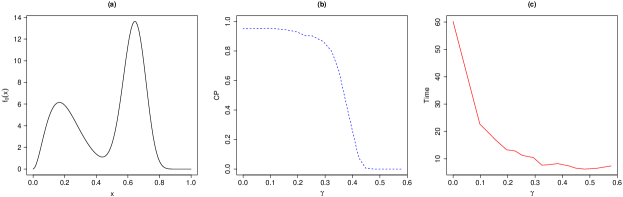
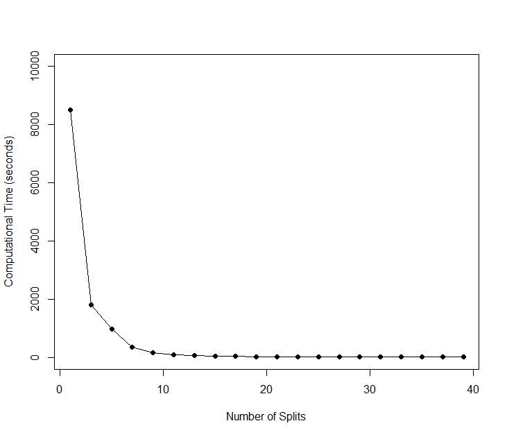
A toy simulation study was carried out to examine the proposed procedures (1)–(3). Specifically, we examine the computing time and coverage probability (CP) of for various choices of . The CP is defined as the relative frequency of the sets that cover the truth. We choose in our GP prior (2.4). Results are summarized in Figure 1. Plot (a) displays the true function under which data were generated. Plot (b) displays how the CP varies as . Plot (c) displays that the computing time decreases when increases. There seems to be a transition for CP vs. , i.e., CP is uniformly close to one when and approaches zero when . In conclusion, possesses both satisfactory frequentist coverage and computational efficiency when . Other choices of either lower CP or slow down the computing. Thus, under a proper choice of , our aggregation procedure can maintain good statistical properties and reduce computing burden at the same time. Careful readers may have noticed that the CP approaches one rather than the credibility level . This issue can be addressed by a modified aggregated set proposed in Section 4.4. More comprehensive simulation results are provided in Section 5 to examine various aggregation procedures such as the pointwise credible intervals.
3 A Nonparametric Bayesian Framework Based on General Design and Space
In this section, we introduce a more general Bayesian nonparametric framework based on general design and function space under which the aggregation results will be obtained. Suppose that the data follow a nonparametric regression model:
| (3.1) |
where is a probability density on , and belongs to an -order Sobolev space :
| (3.2) |
In particular, is a proper subset of . Throughout, we let such that is a reproducing kernel Hilbert space (RKHS). For technical convenience, assume and . When is unknown, our approach can still be applied with replaced by its consistent estimate.
For any , define and . Following [32], there exists a sequence of eigenfunctions and a sequence of eigenvalues such that and
| (3.3) |
where is the Kronecker’s delta.
We next place a prior distribution on , where is a probability measure on and is a hyperparameter. Similar to Section 2, we will characterize through its Radon-Nikodym (RN) derivative w.r.t. , with a pre-given probability measure on . Specifically, assume that the RN derivative of w.r.t. satisfies
| (3.4) |
where is defined in (2.3). Interestingly, it is possible to explicitly construct and such that (3.4) holds. To see this, let
| (3.5) |
where ’s are independent of the observations satisfying . Let . Suppose and are probability measures induced by and , i.e., and for any measurable . It follows by Hájek’s lemma (see [33]) that (3.4) holds. In (3.5), and are both hyper-parameters characterizing the smoothness of the prior. It is easy to check that the sample path of belongs to for any almost surely. As demonstrated in a simulation study, the GCV-selected is sufficient to provide satisfactory results.
4 Main Results
In this section, we present a series of main results that are built upon a uniform Gaussian approximation theorem (Section 4.1). Three classes of aggregation procedures are then proposed: aggregated credible balls in both strong and weak topology, and aggregated credible intervals for linear functionals. These results can be classified into two types: finite sample construction (Sections 4.3, 4.4 and 4.5) and asymptotic construction (Section 4.6). The former construction is often time-consuming since its radius (interval length) is obtained through posterior sampling, while the latter employs a large-sample limit of the radius given by an explicit formula. The computational gain will be illustrated by the simulations in Section 5. Similar to Section 2, let be a random partition of such that with for and .
4.1 A Uniform Gaussian Approximation Theorem
A fundamental theory underlying Bayesian aggregation is developed in this section. It is a uniform version of Gaussian approximation theorem that characterizes the limit shapes of a sequence of individual posterior distributions. This uniform validity holds if the number of posterior distributions does not grow too fast. Also, Bayesian aggregation procedures possess frequentist validity if is chosen properly.
Similar to (2.7), we note that each sub-posterior distribution can be written as
where . Define
| (4.1) |
Suppose that admits the following Fourier expansion:
| (4.2) |
Define with . We remark that is an optimal choice for our aggregation procedure as will be shown later.
Theorem 4.1.
(Uniform Gaussian Approximation) Suppose that admits a Fourier expansion which further satisfies
If the following holds
| (4.3) |
then we have as ,
| (4.4) |
where is the Borel -algebra on with respect to , and ’s are GPs defined by
| (4.5) |
Proof of Theorem 4.1 is rooted in [33] who essentially considered . Substantial efforts have been made here to quantify a range of partition size such that local posteriors can be uniformly approximated by GPs. The explicit structure of the GPs provides a guideline for our aggregation procedures which will be introduced in subsequent sections. It should be emphasized that our aggregation of GPs is weighted-averaging which is different from product-based ones such as [9].
Condition (S) amounts to requiring known regularity of the truth . This can be seen from the inequality since . This condition essentially means that has derivatives up to order (when this order is integer-valued). Combined with (4.3) this means that the regularity of belongs to , i.e., the truth function is jointly confined by both functional space and the prior. The -norm used in (4.5) is defined as follows. For any , define
| (4.6) |
and its squared norm . Clearly, is a valid inner product on .
Remark 4.1.
We remark that (4.3) can be replaced by a more general rate condition:
where . Here, we provide a technical explanation for the terms . Specifically, can be viewed as the rate of convergence of local ordinary penalized MLE (4.1), can be viewed as the posterior contraction rate of the local Bayesian mode, are error bounds of the higher-order remainders in the Taylor expansions of the individual penalized likelihood functions. Uniform Gaussian approximation for general (not necessarily ) can be established under such condition.
Theorem 3.5 in [33] shows that (conditional on ) is induced by a Gaussian process, denoted as , in the sense that for any . Define
| (4.7) |
Then we have
where , and . For convenience, define the mean functions of as
| (4.8) |
such that we can re-express as
where is a zero-mean GP. Note that the posterior mode is very close to since uniformly for ; see the proof of Theorem 4.3. The above characterization of is useful for the subsequent Bayesian aggregation procedures.
4.2 Aggregated posterior means
In this section, we propose a method to aggregate the posterior means , for . The aggregated mean function, denoted as , can be viewed as a nonparametric Bayesian estimate of , and will be used to construct aggregated credible balls/intervals to be introduced later.
Our aggregation procedure is
| (4.9) |
Note that when the model is Gaussian and , (4.9) becomes (2.10). Next we will show that the aggregation procedure (4.9) yields minimax optimality in the following theorem.
Theorem 4.2.
Under conditions of Theorem 4.1, the following result holds:
| (4.10) |
If, in addition, and satisfies
| (4.11) |
then it holds that
| (4.12) |
where denotes the -norm.
4.3 Aggregated credible region in strong topology
In this section, we construct an aggregated credible region based on individual credible regions (w.r.t. a weighted -norm). Specifically, radii are combined in an explicit manner. This aggregated region possesses nominal posterior mass asymptotically, and is further proven to cover the true function with probability tending to one. This nice frequentist property is achieved as long as is not diverging fast and the assigned GP prior in each subset is chosen by setting , i.e., . The conservative frequentist coverage can be improved to the nominal level if we use a weaker norm in defining credible region; see Section 4.4.
Based on each subset , the individual credible ball is constructed as follows:
The credible ball centers around the posterior mean , while its radius is directly sampled from MCMC such that for any . We will construct an “aggregated” region centering at with radius explicitly constructed as follows:
| (4.13) |
where
The final aggregated credible region is obtained as
| (4.14) |
Our theorem below confirms that indeed possesses (asymptotic) posterior mass , and more importantly, proves that it covers the true function with probability tending to one.
Theorem 4.3.
Suppose that satisfies Condition (S), , , , (4.11) and . Then for any , and .
4.4 Aggregated credible region in weak topology
In this section, we invoke a weaker norm (than that used in Section 4.3) to construct an aggregated credible region. Under this new norm (inspired by [5, 6]), it is proven that the frequentist coverage exactly matches with the asymptotic credibility level. The requirement on and in this section remains the same as Section 4.3.
We define a weaker norm than , denoted . For any with , define , where for some constant . Since for all , we have . Under the new -norm, each individual credible region is constructed as
where is directly obtained from posterior sampling such that .
Under -norm, the aggregated credible region is constructed as:
| (4.15) |
where the radius is given as
| (4.16) |
Interestingly, Section 4.6 illustrates that the aggregated radius contracts at root- rate.
Our theorem below shows that the frequentist covergage of exactly matches with the asymptotic posterior mass, both of which achieve the nominal level .
Theorem 4.4.
Suppose that satisfies Condition (S), , , , , and . Then for any , and .
4.5 Aggregated credible interval for linear functional
In this section, we construct aggregated credible intervals for a class of linear functionals of , denoted as . Examples include the evaluation functional, i.e., , and integral functional, i.e., . Specifically, the interval is centered at with an length aggregated through lengths obtained from posterior sampling. Posterior and frequentist coverage properties of this aggregated interval depends on the functional form . Again, our theory holds when is mildly diverging and .
Let be a linear -measurable functional satisfying the following Condition (F): , and there exist constants and such that for any ,
| (4.17) |
It follows by [33] that the evaluation functional satisfies Condition (F) with and the integral functional satisfies Condition (F) with .
Based on each , we obtain from posterior samples the following credible interval:
where is a radius such that . The aggregated credible interval is constructed as
| (4.18) |
where
| (4.19) |
The shrinking rate of depends on the functional form ; see Section 4.6.
Our theorem below investigates the asymptotic properties of in terms of both posterior and frequentist coverage.
Theorem 4.5.
Suppose that satisfies Condition (S′): , a.s. for some constant , for , , , , , (4.11) and . Then for any , , and given that Condition (F) holds. Moreover, if , then .
4.6 Asymptotic aggregated inference
In practice, the centers , and the radii , , in Sections 4.3 – 4.5 are directly obtained from posterior samples. Sometimes posterior sampling is time consuming and inefficient, particularly as . This computational consideration motivates us to propose an asymptotic approach in which one replaces the above centers/radii by their large sample limits. Our new asymptotic inference procedures dramatically improve the computing speed, as displayed in simulations; see Section 5.
Define
| (4.20) |
Clearly, is a counterpart of (4.9) with therein replaced by . By a careful examination of the proofs of Theorems 4.3 – 4.5, it can be shown that the following limits hold:
| (4.21) |
where with being the c.d.f. of standard normal random variable, and satisfies with being independent standard normal random variables.
It yields from (4.6) that the following approximation relationships hold uniformly for :
which further implies (by the aggregation formulae (4.13), (4.16) and (4.19))
| (4.22) | |||
Thus, we have the following asymptotic counterparts of , and :
| (4.23) | |||
| (4.24) | |||
| (4.25) |
Our theorem below shows that the posterior coverage and frequentist coverage of the above computationally efficient alternatives remain the same as those for , and under the same set of conditions.
Theorem 4.6.
As a byproduct, (4.22) implies the contraction rate of each aggregated credible ball/interval in Sections 4.3 – 4.6. It is easy to see that . As for , it depends on the functional form . For example, when is an evaluation functional, it holds that , leading to when ; when is an integral functional, we have since . As for , it can be shown by a simple fact that when . This contraction rate turns out to be optimal based on the entire sample; see [39]. However, if we choose in the scale of subsample size , e.g., , similar arguments show that . Hence, such a region contracts faster than the optimal rate, which results in unsatisfactory frequentist coverage.
Table 1 summarizes six aggregated credible regions/intervals from Sections 4.3 – 4.5 in terms of their centers and radii.
| Type | Name | Notation | Center | Radius |
|---|---|---|---|---|
| Finite-sample | strong CR for | |||
| weak CR for | ||||
| CI for | ||||
| Asymptotic | strong CR for | |||
| weak CR for | ||||
| CI for |
5 Simulation Study
In this section, statistical properties of the proposed aggregated procedures are examined using a simulation study. We generated samples from the following model
| (5.1) |
where , , and are independent of . The true regression function was chosen to be , where is the probability density function for .
Consider GP prior , where are defined in (3.5). The proposed Bayesian procedures were examined. Specifically, we computed the frequentist coverage proportions (CP) of the credible regions (4.14), (4.15), (4.23), (4.24), and credible intervals (4.18), (4.25). In particular, (4.14), (4.15) and (4.18) were constructed based on posterior samples, as described in Sections 4.2–4.5; whereas (4.23), (4.24) and (4.25) were constructed based on asymptotic theory developed in Section 4.6. To ease presentation, we call (4.14) and (4.15) as finite-sample credible regions (FCR), and call (4.23) and (4.24) as asymptotic credible regions (ACR).
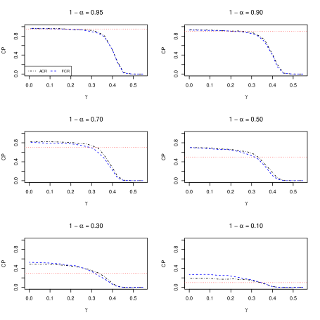
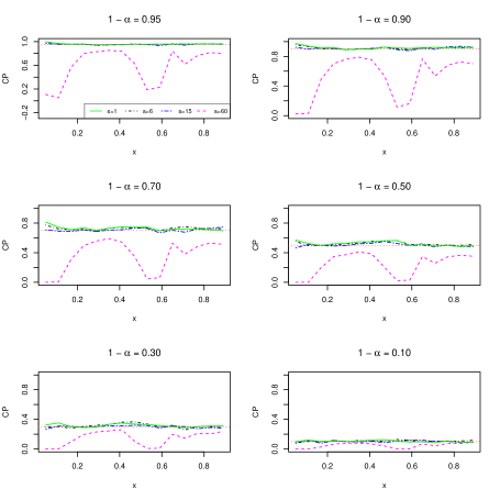
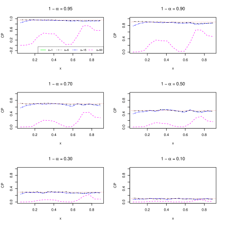
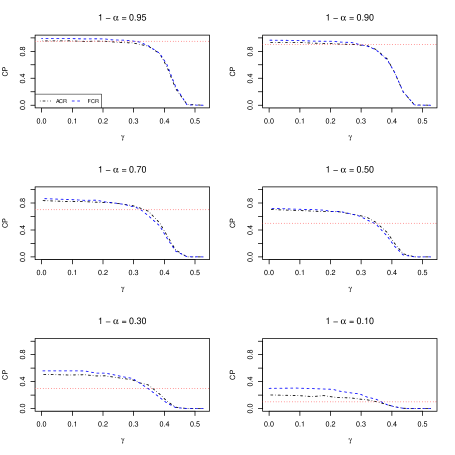
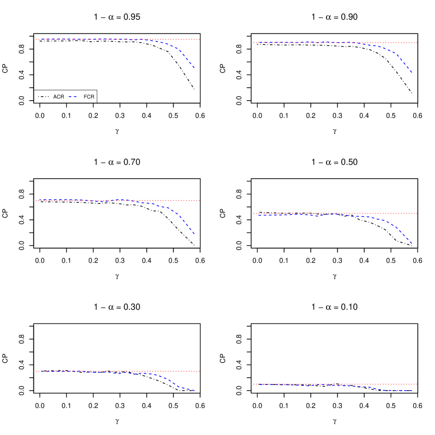
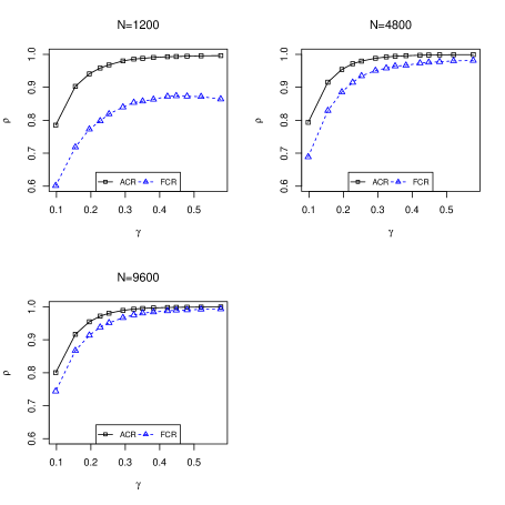
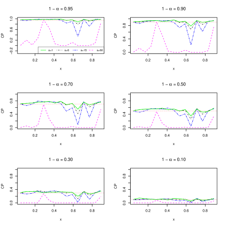
The calculation of CP was based on independent experiments. Specifically, the CP is the proportion of the credible regions/intervals containing / (for a linear functional ). Two types of were considered: (1) the evaluation functional for any , and (2) the integral functional for any . In both cases, we consider with being 15 evenly spaced points in [0.05,0.95]. To make the study more complete, a set of credibility levels were examined, i.e., . In each experiment, independent samples were generated from the model (5.1). For ACR and FCR, we chose the number of divisions . Define . Note that (equivalently, ) means “no division.”
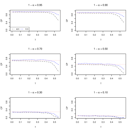
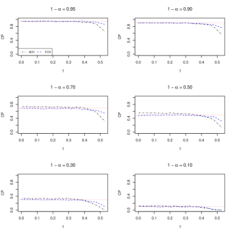
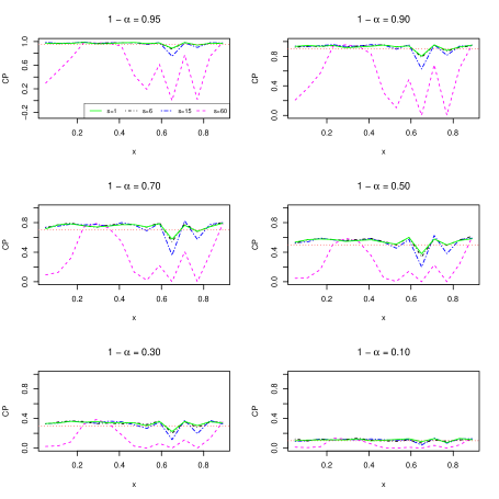
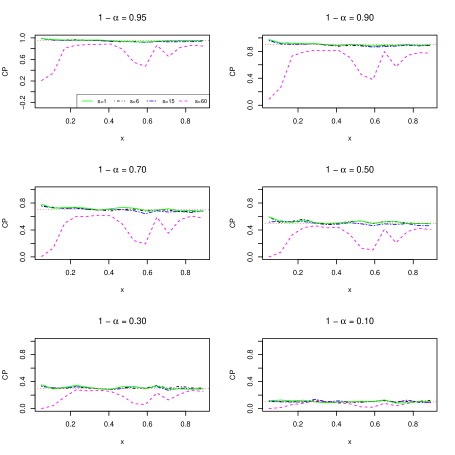
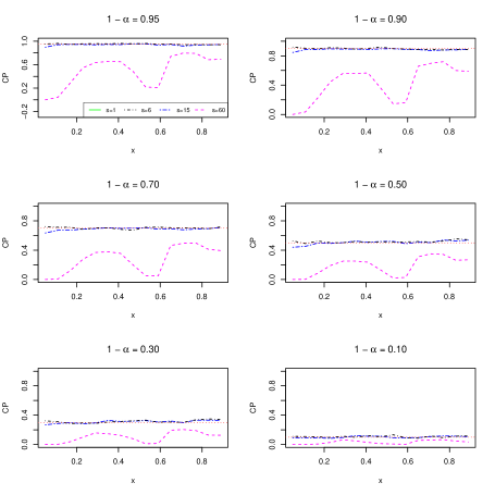
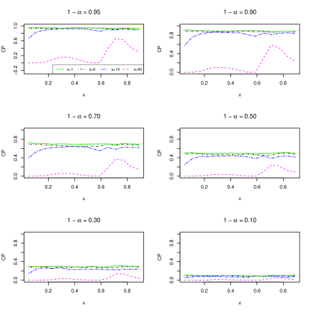
Figure 2 demonstrates the results for FCR and ACR based on strong topology, i.e., (4.14) and (4.23). The red dotted line indicates the credibility level. It can be seen that the CP of both FCR and ACR is above the credibility levels when is small, while it suddenly drops to zero as is beyond some threshold, say . This observation supports our theory that should not grow too fast, and that the credible regions based on strong topology tends to be more “conservative.” Figure 3 demonstrates the results for FCR and ACR based on weak topology, i.e., (4.15) and (4.24). We observe that the CP of both ACR and FCR approaches the desired credibility levels when , but quickly drops to zero when becomes large. This observation also supports our theory that the use of weak topology leads to a more satisfactory frequentist coverage.

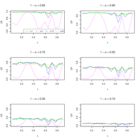
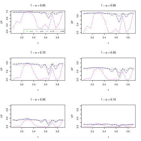
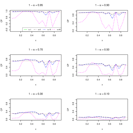
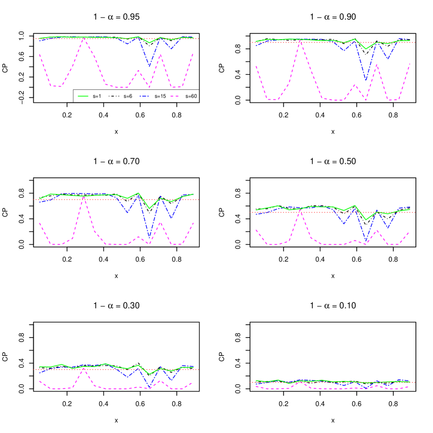
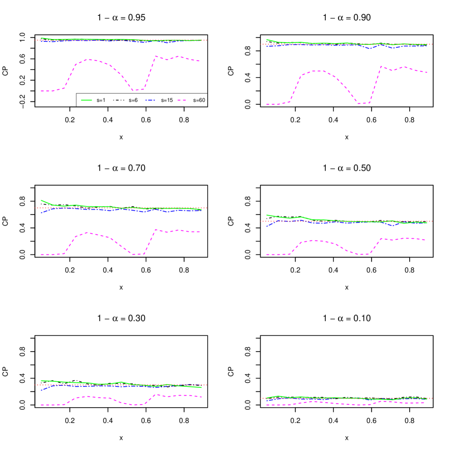
For credible intervals of linear functionals, we chose the number of divisions . Figures 4 and 5 display the results for evaluation functional and integral functional, respectively, based on posterior samples. It can be seen that when , the CP of the credible intervals for the evaluation functional drops to zero at most of the points, indicating the failure in covering the true values of the function. However, when , the CP is above the credibility levels except for the points where the true function has peaks; see (a) of Figure 1. The observation that the CP stays above coincides with our theory that the credible interval of the evaluation functional is conservative. On the other hand, it can be seen that when , the CP of the credible intervals for the integral functional becomes far below the credibility levels at most . However, when , the CP is close to the credibility levels at all . This finding coincides with our theory that the the credible interval of the integral functional achieves exactly frequentist coverage. The above results also support our claim that cannot grow too fast for guaranteeing frequency validity. Credible intervals based on asymptotic theory, i.e., (4.25), were summarized in Figures 11 and 12 of the supplement document [34]. Interpretations of these results are similar to those based on finite posterior samples.
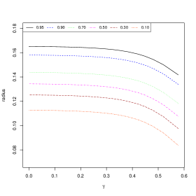
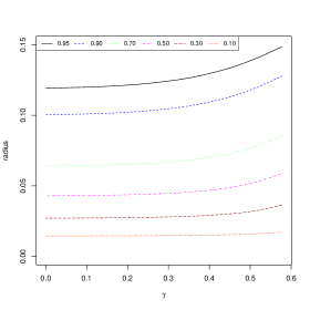
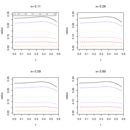
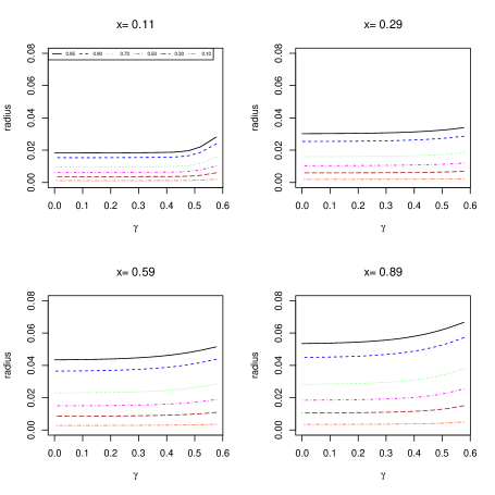
The supplement document [34] also includes Figures 13 – 16 which demonstrate how the radii/lengths of the aggregated credible regions/intervals change along with , the size of the subsample. It can be observed that when , indicating that the full sample is divided into at most twelve subsamples, the radii of the aggregated regions/intervals are almost identical to the radii of the regions/intervals directly constructed from the full sample, i.e., . This means that our aggregated procedures, based on a suitable amount of divisions, indeed mimic the oracle procedures. However, when increases to , the distinctions between the the aggregated and oracle procedures quickly become obvious.
We also repeated the above study for and . The plots corresponding to these studies are given in supplement document; see Section S.8.6 of [34]. The interpretations of these additional results are similar as above.
To the end of this section, computing efficiency is investigated. Figure 6 displays the results based on a single experiment for various choices of . Specifically, we look at the value of the quantity versus a collection of ’s for FCR and ACR, where () is the computing time without using D&C (based on D&C). We observe that is substantially smaller than , and this computation efficiency (as reflected by the value of ) becomes more obvious as grows for each fixed . This can also be seen as grows for each fixed . However, this reduction in computing time does not affect the performances of the aggregated credible regions when , as demonstrated in Figures 2, 3, 13–16.
6 Real Data Analysis
In this section, we apply our methods to Million Song Data (MSD) and Flight Delay Data (FDD).
6.1 Million Song Data
As a real application, we apply our aggregation procedure to analyze MSD. The MSD is a perfect example of large dataset, a freely-available collection of audio features and metadata for a million contemporary popular music tracks. Each observation is a song track released between the year 1922 and 2011. The response variable is the year when the song was released and the covariate is the timbre average of the song. The main purpose is to explore a relationship, denoted as , between song features and years in a nonparametric regression model, i.e., +error. The above model is useful to predict production year based on song timbre. Due to enormous sample size, processing the entire data is infeasible. In frequentist setting, a distributed kernel ridge regression method was proposed by [46, 48] for estimation purposes (without quantifying uncertainty).
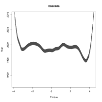
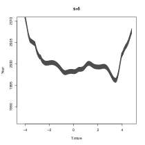
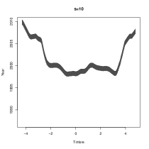
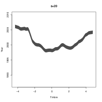
In the Bayesian setup, we applied our aggregation procedure to construct 95% credible sets for based on a subset of songs released from the year 1996 to 2010. We randomly split the observations to subsets. We also compared our results with the baseline method in which all ten thousand observations were used. Credible sets are displayed as gray areas in Figure 7. We find that the shapes of all credible sets are overall the same when the timbre ranges from -4 to 4, e.g., all display a W-shape, although the results are a bit sensitive near the endpoints. Therefore, the overall pattern of the sets appears to be insensitive to the above selections of .
6.2 Flight Delay Data
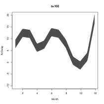
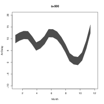
We applied our aggregation procedure to one more real data set, the FDD. The data consists of flight arrival and departure information for all commercial flights within the United States, from October 1987 to April 2008. The main purpose is to find the key factors that have an impact on the flight delay. We considered the relationship (denoted ) between month and the length of the flight delay, i.e., +error. Negative length of delay implies that the flight arrived earlier. We applied the same Bayesian aggregation procedure as described in MSD to a randomly selected subset of flight information in the year 2007. We randomly split the observations to subsamples, based on which the aggregated credible sets for were constructed. We also compared the results with the baseline where all the ten thousand samples were used. Credible sets are displayed as gray areas in Figure 8. Again, the shapes of the four credible sets appear to be almost the same for all .


6.3 Computation Efficiency
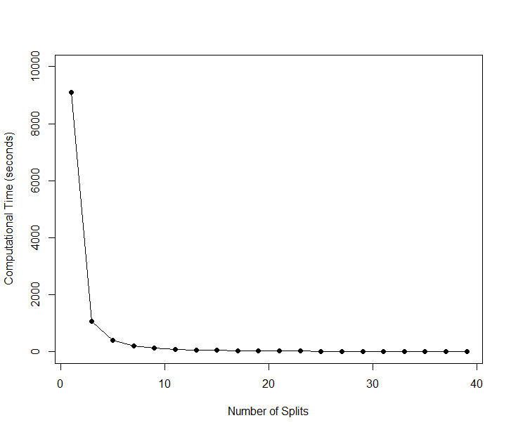
We compare the overall execute computation time of both MSD and FDD on different numbers of splits, e.g. computational time per machine number of machines in Figure 9-10. It can be seen that the computing time dramatically decreases as the number of splits increases, which reflects the scalability of our proposed algorithm.
7 Conclusions
This paper proposes algorithms for aggregating individual posterior results such as modes, balls, intervals, into their global counterparts. The algorithms are easy-to-implement which are particularly useful in big data scenarios. We also experimented the proposed algorithms through simulated and real data sets. A notable contribution of this article is to provide rigorously justified theoretical guarantees. The major tool for proving our theoretical results is a uniform Gaussian approximation theorem which shows that the individual posterior distributions converge uniformly to Gaussian processes provided that the number of subsets is not too large.
Acknowledgments
Shang’s research is sponsored by NSF DMS-1764280 and NSF DMS-1821157. Cheng’s research is sponsored by NSF (CAREER Award DMS-1151692, DMS-1418042) and Office of Naval Research (ONR N00014-15-1-2331). The authors thank the Associate Editor Eric P. Xing and two anonymous referees for their helpful comments and suggestions that significantly improve the quality of this paper.
8 APPENDIX
This appendix section contains the proofs of the main results. Section A.1 contains proof of Theorem 4.1 and relevant preliminary results. Section A.2 includes the proof of Theorem 4.2. Sections A.3 and 4.4 includes the proofs of Theorems 4.3 and 4.4, i.e., coverage properties of the credible sets based on strong and weak topology respectively.
All proofs crucially depend on an eigensystem designed for simultaneous diagonalization of the two bilinear functionals induced from likelihood and prior, respectively. In fact, is a solution of the following ordinary differential system (whose existence and uniqueness is guaranteed by [2]):
| (A.1) |
Properties of this eigen-system are summarized in Proposition A.1, whose proof can be found in [32, Proposition 2.2].
Proposition A.1.
It holds that , and that the sequence is nondecreasing with , and for . Moreover, and
| (A.2) |
where is the Kronecker’s delta. In particular, any admits a Fourier expansion with convergence held in the -norm.
A.1 Proofs in Section 4.1
The proof of Theorem 4.1 requires the following technical result which derives a local contraction rate uniformly over : . The proof can be found in ([34]).
Proposition 8.1.
If satisfies Condition (S) and the following Rate Condition (R) holds:
Let be a fixed constant. Then for any , there exist positive constants s.t. for any ,
| (A.3) |
Proof of Theorem 4.1.
Let be large positive constants. For any fixed constant , consider three events:
where means expectation taken under . It follows from [34] and Proposition 8.1 that we can choose (both large enough) s.t. where is an arbitrary constant. Meanwhile, by ([34]) we have, on , for any ,
| (A.4) | |||||
where is a universal constant and . We can choose so that the quantity (A.4) is less than . So implies , so that . Define , then it can be seen that .
Let be defined as
| (A.5) |
Following Lemma S.6, for any ,
| (A.6) |
It follows from the proof of Proposition 8.1 that on , for any satisfying and ,
| (A.7) |
where is a positive constant depending only on . Recall that our assumption says that .
For , define
For simplicity, let . On (with ) and for any ,
By some algebra, it can be shown that the above inequalities lead to
| (A.8) |
Meanwhile, on and for any , using (A.7) and the elementary inequality for , we get that
leading to that
| (A.9) |
Combining (A.8) and (A.9), on and for any , . When is large, and both quantities are small, the above inequalities lead to
| (A.10) |
For simplicity, denote . For any , let . Then on , we get that . Moreover, it follows from (A.10) that on and for any ,
Note that the right hand side is free of . Then we get that on , . This implies that for sufficiently large ,
The desirable result follows by the simple fact when . ∎
A.2 Proofs in Section 4.2
Proof of Theorem 4.2.
We first show (4.10). Let and for . By Proposition 8.1, Theorem 4.1 and (A.4) with therein, we can choose sufficiently large such that
where the second last equality uses Theorem 4.1 and the fact that, uniformly for ,
Then (4.10) follows from the trivial fact that .
Next we show (4.12). By direct examinations we can verify the following Rate Conditions (R):
It is easy to see that for all . Then it holds from (4.20) that
| (A.11) | |||||
The last equality owes to the condition and .
By direct examinations, we have
| (A.12) | |||||
Denote the four terms in the above equation by .
Since , it is easy to see that
A.3 Proofs in Section 4.3
Before proving Theorem 4.3, we give some preliminary notation and results. Define an “oracle” penalized likelihood . Applying Theorem 4.1 to , we have
| (A.14) |
where and is the “oracle” smoothing spline estimator based on full data. Consider a generalized Fourier expansion of : . By Theorem 5.2 in [33], we have for any , where . Here, are analogous to ones in the definition of in Section 4.1, and and are given in (4.7). Define the mean functions of as . So we can re-express as , where is a zero-mean GP.
The following result describes the distribution of and .
Lemma A.1.
As , .
Proof of Theorem 4.3.
We can show that Rate Conditions (R) hold by direct calculations.
It is sufficient to investigate the -probability of the event . To achieve this goal, we first prove the following fact:
| (A.15) |
where and is the c.d.f. of , and . The proof of the theorem follows by (A.15) and a careful analysis of .
We first show (A.15). It follows by Theorem 4.1 that for any ,
Together with , we have . Let for . It is clear that
| (A.16) | |||||
and, for any ,
| (A.17) | |||||
and by Theorem 4.2, , where . By (4.11), (Lemma A.1), and direct examinations it holds that
| (A.18) |
Combining (A.16) and (A.17) we get that
where is the c.d.f. of . It follows by Lemma A.1 and Polya’s theorem ([10]) that uniformly converges to , the c.d.f. of standard normal variable. Therefore, when becomes large enough,
where implies that
Since (A.18) implies that and are both uniformly for , so (A.15) holds.
Next we prove the theorem. Consider expansion (A.12). Only focus on . Define . Let , then . Note that is clean in the sense of [11]. Let and , , be defined as , , and
Since are uniformly bounded, we get that , where “” is free of . This implies that and .
It can also be shown that for pairwise distinct ,
which implies that . In the mean time, a straight algebra leads to that
Since , we get that and are all of order . Then it follows by [11] that as , . Since , the above equation leads to that .
It follows by direct examination that , leading to that . Therefore, it follows by Rate Condition (R), i.e., , and the analysis on in (A.12) that
| (A.19) |
In the end, note from (A.15) and for (see proof of Lemma A.1) that , which leads to that
| (A.20) |
Therefore, . Since , we get by (A.11) that, with -probability approaching one, . Meanwhile, it follows by [34] that and , where . Note that , which leads to . Since , we get that
Using (A.11) we get that . Since , we have that . It follows by , (A.14) and (A.20) that . This completes the proof. ∎
A.4 Proofs in Section 4.4
Before proving Theorem 4.4, let us present a preliminary lemma.
Lemma A.2.
As , , where are independent standard normal random variables.
Proof of Theorem 4.4.
By direct examinations, one can show that Rate Conditions (): , , and are all satisfied.
We first have the following fact:
| (A.22) |
where satisfies with being independent standard normal random variables. It follows from (A.22) that
| (A.23) |
By Theorem 4.2 and the condition we have the following . Also, for arbitrarily small , . The proof of (A.22) is then similar to the proof of (A.15) and details are omitted.
Let be defined in (A.12). It follows from the proof of Theorem 4.3 that , so due to the condition . It follows by condition , dominated convergence theorem and direct examinations,
and
A.5 Computational Details
In this subsection, we provide some computational details relating to Section 2.2. For convenience, we rewrite model (2.1) as following:
Calculation of posterior means. In order to calculate the posterior mean , we have to generate samples of from its posterior distribution . In practice, directly sampling the function from is impossible. Instead, we generate some samples from . As is large, can represent the whole curve of . Firstly, let us derive the posterior distribution for . For the -th subsample, the likelihood function is written by
Since follows a GP prior with mean zero and covariance function , where is given in (2.5), the prior of is multivariate Gaussian:
where is the covariance matrix satisfying
involves an infinite summation which is practically infeasible. Instead, the infinite sum is approximated by a finite one, i.e.,
In our numerical study, we found that can already provide a good approximation. Due to the conjugacy, the posterior distribution of also follows a multivariate Gaussian distribution
Next we generate independent samples, denoted from above multivariate Gaussian distribution. Therefore, the posterior mean can be approximated by
Calculation of posterior radius. Once we have independent samples , we are able to approximate by
Finally, the radius is approximated by the upper -th percentile of .
References
- [1] Adams, R. A. (1975). Sobolev Spaces. Academic Press, New York-London. Pure and Applied Mathematics, Vol. 65.
- [2] Birkhoff, D. (1908). Boundary value and expansion problems of ordinary linear differential equations. Transactions of the American Mathematical Society, 9, 373–395.
- [3] Hunt, B. R., Sauer, T. and Yorke, J. A. (1992). Prevalence: a translation-invariant “almost every” on infinite-dimensional spaces. Bulletin of the American Mathematical Society, 27, 217â-238.
- [4] Cameron, R. H. and Martin, W. T. (1944). Transformations of Wiener integrals under translations. Annals of Mathematics, 45, 386–396.
- [5] Castillo, I. and Nickl, R. (2013). Nonparametric Bernstein-von Mises theorem in Gaussian white noise. Annals of Statistics, 41, 1999–2028.
- [6] Castillo, I. and Nickl, R. (2014). On the Bernstein-von Mises phenomenon for nonparametric Bayes procedures. 42, 1941–1969.
- [7] Huang, Zaijing and Gelman, Andrew (2005). Sampling for Bayesian computation with large datasets.
- [8] Neiswanger, Willie and Wang, Chong and Xing, Eric P. (2014). Asymptotically Exact, Embarrassingly Parallel MCMC. Proceedings of the Thirtieth Conference on Uncertainty in Artificial Intelligence.
- [9] Cao, Yanshuai and Fleet, David J (2014). Generalized product of experts for automatic and principled fusion of Gaussian process predictions. arXiv preprint arXiv:1410.7827.
- [10] Chow, Y. and Teicher, H. (1988). Probability Theory, 3rd Ed. Springer, New York.
- [11] de Jong, P. (1987). A central limit theorem for generalized quadratic forms. Probability Theory & Related Fields, 75, 261–277.
- [12] Eggermont, P. P. B. and LaRiccia, V. N. (2009). Maximum Penalized Likelihood Estimation: Volume II. Springer Series in Statistics.
- [13] Ghosal, S., Ghosh, J. K. and van der Vaart, A. W. (2000). Convergence rates of posterior distributions. Annals of Statistics, 28, 500–531.
- [14] Hájek, J. (1962). On linear statistical problems in stochastic processes. Czechoslovak Mathematical Journal, 12, 404–444.
- [15] Hoffmann-Jorgensen, Shepp, L. A. and Dudley, R. M. (1979). On the lower tail of Gaussian seminorms. Annals of Probability, 7, 193–384.
- [16] Kuelbs, J., Li, W. V. and Linde, W. (1994). The Gaussian measure of shifted Probability Theory & Related Fields, 98, 143-â162.
- [17] Kleiner, A., Talwalkar, A., Sarkar, P. and Jordan, M. (2012). Bootstrapping big data. In Proceedings of the 29th International Conference on Machine Learning.
- [18] Kosorok, M. R. (2008). Introduction to Empirical Processes and Semiparametric Inference. Springer: New
- [19] Li, C., Srivastava, S. and Dunson, D. B. (2017). Simple, Scalable and accurate posterior interval estimation. Biometrika, 104, 665–680.
- [20] Szabó, B. and van Zanten, H. (2017). An asymptotic analysis of distributed nonparametric methods. arxiv.org/abs/1711.03149.
- [21] Szabó, B. and van Zanten, H. (2017). Adaptive distributed methods under communication constraints. arxiv.org/abs/1804.00864.
- [22] Srivastava, S., Li, C. and Dunson, D. B. (2018). Scalable Bayes via barycenter in Wasserstein space. Journal of Machine Learning Research, 19, 1–35.
- [23] Li, W. V. (1999). A Gaussian correlation inequality and its applications to small ball probabilities. Electronic Communications in Probability, 4, 111–118.
- [24] McDonald, R., Hall, K., and Mann. G. (2010). Distributed training strategies for the structured perceptron. In North American Chapter of the Association for Computational Linguistics (NAACL).
- [25] Minsker, S., Srivastava, S., Lin, L. and Dunson, D. (2017). Robust and scalable Bayes via a median of subset posterior measures. Journal of Machine Learning Research, 18, 1–40.
- [26] Morris, C. N. (1982). Natural exponential families with quadratic variance functions. Annals of Statistics, 10, 65–80.
- [27] Messer, K. and Goldstein, L. (1993). A new class of kernels for nonparametric curve estimation. Annals of Statistics, 21, 179–195.
- [28] Pinelis, I. (1994). Optimum bounds for the distributions of martingales in Annals of Probability, 22, 1679–1706.
- [29] Rudin, W. (1976). Principles of Mathematical Analysis. McGraw-Hill. New York.
- [30] Rivoirard, V. and Rousseau, J. (2012). Bernstein-von Mises theorem for linear functionals of the density. Annals of Statistics, 40, 1489–1523.
- [31] Steven L. Scott and Alexander W. Blocker and Fernando V. Bonassi and Hugh A. Chipman and Edward I. George and Robert E. McCulloch (2016). Bayes and Big Data: The Consensus Monte Carlo Algorithm. International Journal of Management Science and Engineering Management.
- [32] Shang, Z. and Cheng, G. (2013). Local and global asymptotic inference in smoothing spline models. Annals of Statistics, 41, 2608–2638.
- [33] Shang, Z. and Cheng, G. (2018). Gaussian Approximation of General Nonparametric Posterior Distributions. Information and Inference: A Journal of the IMA, 7, 509–529.
- [34] Shang, Z., Hao, B. and Cheng, G. Supplementary document to “Nonparametric Bayesian Aggregation for Massive Data.”
- [35] Srivastava, S., Li, C. and Dunson, D. B. (2015). Scalable Bayes via Barycenter in Wasserstein Space. Preprint. http://arxiv.org/abs/1508.05880.
- [36] van den Boom, W., Reeves, G. and Dunson, D. (2015). Scalable Approximations of Marginal Posteriors in Variable Selection. Preprint. http://arxiv.org/abs/1506.06629
- [37] van der Geer, S. A. (2000). Empirical Processes in M-Estimation. Cambridge University Press, New York.
- [38] van der Vaart, A. W. and van Zanten, J. H. (2008). Reproducing kernel Hilbert spaces of Gaussian priors. IMS Collections. Publishing the Limits of Contemporary Statistics: Contributions in Honor of Jayanta K. Ghosh. 3, 200–222.
- [39] van der Vaart, A. W. and van Zanten, J. H. (2008). Rates of contraction of posterior distributions based on Gaussian process priors. Annals of Statistics, 36, 1031–1508.
- [40] Wahba, G. (1985). A comparison of GCV and GML for choosing the smoothing parameter in the generalized spline smoothing problem. Annals of Statistics, 13, 1251–1638.
- [41] Wahba, G. (1990). Spline Models for Observational Data. SIAM, Philidelphia.
- [42] Weinberger, H.F. (1974). Variational methods for eigenvalue approximation. CBMS-NSF Regional Conference Series in Applied Mathematics.
- [43] Wang, X. and Dunson, D. (2014). Parallelizing MCMC via Weierstrass Sampler. Preprint. http://arxiv.org/abs/1312.4605
- [44] Wang, X., Guo, F., Heller, K. A. and Dunson, D. (2015). Parallelizing MCMC with Random Partition Trees. Neural Information Processing System (NIPS’15).
- [45] Wang, X., Peng, P. and Dunson, D. (2014). Median Selection Subset Aggregation for Parallel Inference. Neural Information Processing System (NIPS’14).
- [46] Zhang Y., Duchi, J. and Wainwright, M. J. (2015). Divide and Conquer Kernel Ridge Regression: A Distributed Algorithm with Minimax Optimal Rates. Journal of Machine Learning Research, 16, 3299–3340.
- [47] Zhao, T., Cheng, G. and Liu, H. (2015). A Partially Linear Framework for Massive Heterogeneous Data. Annals of Statistics, 44, 1400–1437.
- [48] Zhang, Y., Wainwright, M. J. and Jordan, M. I. (2015). Distributed Estimation of Generalized Matrix Rank: Efficient Algorithms and Lower Bounds. International Conference on Machine Learning (ICML’15).
Supplementary document to
This supplementary document is structured as follows.
- •
- •
- •
-
•
Section S.8.5 includes a result that characterizes the posterior tail moments of for any .
- •
S.8.1 Proofs of Lemmas A.1 and A.2
Proof of Lemma A.1.
We only show the first limit distribution since the proof of the second one is similar.
Let . Then is a sequence of iid standard normals. Note that
Let , then we have
By straightforward calculations and Taylor’s expansion of , it can be shown that the logarithm of the moment generating function of equals
| (S.1) |
Proof of Lemma A.2.
The proof follows by moment generating function approach and direct calculations. ∎
S.8.2 Proofs in Sections 4.5 and 4.6
Proofs in Section 4.5
Proof of Theorem 4.5.
Recall in the proof of Theorem 4.4 we showed that Rate Conditions () are satisfied.
It is easy to see that
| (S.2) |
For , define . It follows by Theorem 4.1 that . Since , it can be examined that . Together with the condition and the fact , one can verify that . So we have by (4.17) and Theorem 4.2 that
Combined with (S.2) we get that
The above argument leads to uniformly for , which further leads to the following
| (S.3) |
Consider the decomposition (A.12) with being defined therein. It follows by (A.2) and rate condition that . Meanwhile, it follows by Condition (S′), and and direct examinations that
and
By (A.11) and we get . Therefore, . If follows from (4.17) that .
Note that , where the kernel is defined in the proof of Theorem 4.3. We will derive asymptotic distribution for . Let . It is easy to show that
Clearly, by uniform boundedness of and , we get
where the “” is free of , and
| (S.4) |
Then for any , by condition a.s.,
where the last -term follows by and . By Lindeberg’s central limit theorem, as ,
| (S.5) |
Proofs in Section 4.6
S.8.3 Proofs of Proposition 8.1 and relevant results
The goal of this section is to prove Proposition 8.1 and relevant results. Before proofs, we exactly describe the Fréchet derivatives of the likelihood function that will be technically useful. Suppose that follows model (3.1) based on . Let for . For , the Fréchet derivative of can be identified as
Define . We also use and to represent the second- and third-order Fréchet derivatives of . Note that , and can be expressed as
| (S.9) |
The Fréchet derivative of is denoted . These derivatives can be explicitly written as
The proof of Proposition 8.1 requires a series of preliminary lemmas. Define . We first state a basic lemma about a concentration phenomenon of smoothing spline estimates in the distributed setup.
Lemma S.1.
Lemma S.2.
For any fixed constants and , let
| (S.10) |
| (S.11) |
Then as ,
and
Lemma S.3.
It holds that
| (S.12) |
Lemma S.4.
Under Condition (S), we get .
Proof of Lemma S.4.
Consider a function class
| (S.13) |
Lemma S.5.
For any fixed constant , as ,
where , .
Proof of Lemma S.5.
Lemma S.6.
For ,
-
(1).
, where for any ;
-
(2).
, where recall that (see A.5)
(S.14)
Lemma S.7.
There exists a universal constant s.t.
where recall that is the probability measure induced by .
Proof of Lemma S.7.
Proof of Proposition 8.1.
Fix any . Let be a large constant so that (thanks to Lemma S.4) the event
| (S.15) |
has probability approaching one. Meanwhile, for a fixed constant , define
| (S.16) |
By Lemma S.5 we have that has -probability approaching one. Thus, it holds that, when becomes large, , where . In the rest of the proof we simply assume that holds.
For some positive constant , it follows by Theorem 8.2 that
Let be a constant to be further determined later, then we have that
The first term is . Thus, when is sufficiently large,
for a large constant .
Next we only need to handle the second term. Let . It follows by Lemma S.6 that , and . Therefore,
where .
Let
Then on and for , we have .
Let . It follows by similar arguments as above (S.23) that . Note that on and for , for all ,
| (S.17) | |||||
where is constant depending only on .
It follows that on and for all ,
Since (Lemma S.7), together with , we get that . Therefore, , leading to
| (S.18) |
This implies by rate conditions that, on and for any ,
Next we handle . The idea is similar to how we handle but with technical difference. Let . Note that , and hence, on , for any , i.e., , we get that . Let . Then . Using previous similar arguments handling , we have that on , for any and ,
where is constant only depending on and the last inequality follows by rate condition . It is easy to see that on and for any and , , leading to that
where is the th prior moment of which is finite. Choose to be large such that
Therefore, on ,
So we get that
By , the above leads to that
Proof is completed. ∎
S.8.4 Proofs of other results in Section S.8.3
Let be the -packing number in terms of supremum norm, where recall that the space is defined in (S.13). The following result can be found in [37].
Lemma S.8.
There exists a universal constant s.t. for any ,
For , define . For arbitrary , define
| (S.19) | |||||
where .
We have the following useful lemma.
Lemma S.9.
For any and , suppose that is a measurable function defined upon and satisfying and the following Lipschitz continuity condition: for any and ,
| (S.20) |
Then for any constant and ,
where and
Proof of Lemma S.9.
For any and , and any , we get that
By Theorem 3.5 of [28], for any , . Then by Lemma 8.1 in [18], we have
where denotes the Orlicz norm associated with . Recall . Define . Then it can be shown by elementary calculus that , and for any , . By a careful examination of the proof of Lemma 8.2, it can be shown that for any random variables ,
| (S.21) |
Next we use a “chaining” argument. Let be a sequence of finite nested sets satisfying the following properties:
-
•
for any and any , ; each is “maximal” in the sense that if one adds any point in , then the inequality will fail;
-
•
the cardinality of is upper bounded by
where is absolute constant;
-
•
each element is uniquely linked to an element which satisfies .
For arbitrary with , choose two chains (both being of length ) and with for . The ending points and satisfy
and hence, . It follows by the proof of Theorem 8.4 of [18] and (S.21) that
On the other hand,
Therefore,
Now for any with . Let , hence, . Since is “maximal”, there exist s.t. . It is easy to see that . So
Therefore, letting we get that
Taking in the above inequality, we get that
By Lemma 8.1 in [18], we have
Note that the right hand side in the above does not depend on . This completes the proof. ∎
Proof of Lemma S.1.
Let be the parameter based on which the data are drawn. It is easy to see that . Therefore, for any , , implying .
The proof of (a) is finished in two parts.
Part I: For any , define an operator mapping to :
First observe that, under with ,
Let . Let be the -ball. For any , using , it is easy to see that . Therefore, maps to itself. For any , by Taylor’s expansion we have
This shows that is a contraction mapping which maps into . By contraction mapping theorem (see [29]), has a unique fixed point satisfying . Let . Then and .
Part II: For any , under (3.1) with being the truth, let be the function obtained in Part I s.t. . Define an operator
Rewrite as
Denote the above two terms by , respectively.
For any , let . Obviously,
Therefore, which leads to that
where . Let . By condition , we have
It follows by Theorem 3.2 of [28] that, for ,
| (S.22) | |||||
We note that the right hand side in (S.22) does not depend on . Moreover, it is easy to see that . Let
then . Define , and . By Lemma S.9, , where .
For any , let , where . It follows that
Therefore, . Consequently, on , for any , we get , which leads to that
| (S.23) | |||||
where the last inequality follows by condition . Note that the above inequality also holds for .
Let . Therefore, it follows by (S.23) that, for any , on and for any , . Meanwhile, for any , replacing by in (S.23), we get that . Therefore, for any , on , is a contraction mapping from to itself. By contraction mapping theorem, there exists uniquely an element s.t. . Let . Clearly, , and hence, is the maximizer of ; see (4.1). So we get that, on , . The desired conclusion follows by the trivial fact: . Proof of (a) is completed.
Next we show (b).
For any , let be the penalized MLE of obtained by (4.1). Let , , .
On , we have . Let . Clearly, . Then we get that
| (S.24) | |||||
S.8.5 An initial contraction rate
Theorem 8.2 below states that the posterior measures uniformly contract at rate , where recall that . This is an initial rate result that holds irrespective the diverging rate of .
Theorem 8.2.
(An Initial Contraction Rate) Suppose satisfies Condition (S). Let be a fixed constant. If , , , then there exists a universal constant s.t.
as , no matter is fixed or diverges at any rate.
Before proving Theorem 8.2, we present a preliminary lemma.
Let be a bounded orthonormal basis of under usual inner product. For any , define
Then can be viewed as a version of Sobolev space with regularity . Define , a centered GP, and . Define , the usual inner product, , a functional on . For simplicity, denote . Clearly, . Since is a Gaussian process with covariance function
it follows by [38] that is the RKHS of . For any with , define inner product
Let be the norm corresponding to the above inner product. The following lemma is used in the proof of Theorem 8.2. Its proof can be found in [33].
Lemma S.10.
Let be any positive sequence. If Condition (S) holds, then there exists such that
-
(i).
,
-
(ii).
,
-
(iii).
.
To ease reading, we sketch the proof of Theorem 8.2. We first show the following result: for any , as ,
| (S.25) |
To show (S.25), we can rewrite the posterior density of by
where recall that is the probability density of under . For , define
| (S.26) |
| (S.27) |
| (S.28) |
where and , with the quantities specified later. Using LeCam’s uniformly consistent test [13], we will show that is of an exponential order (in the sense of ). Then (S.25) holds by taking in . The proof of Theorem 8.2 will be completed by decomposing into three terms based on an auxiliary event with each term of an exponential order.
Proof of Theorem 8.2.
Note that there exists a universal constant such that for any . Therefore, there exists a universal constant s.t. .
Define . Then
where for any . Define , a reduced probability measure on . By Jensen’s inequality,
For any , . By [SC18, Lemma A.9] and the condition , we can choose to be sufficiently large so that .
It follows by Taylor’s expansion and , that for any ,
Therefore, for any .
Since , we can choose to be large so that . Meanwhile, for any , for some , we have
We have used in the above inequalities.
For any , define . It is easy to check that , as . Define , we get that , a.s. It can also be shown by that, as ,
where is an absolute constant.
Let . Note that by the condition we have , we can let be large so that . Let for , then it is easy to see that
Let . It can be shown using inequality for and Cauchy-Schwartz inequality that
where the last step follows from for any . Therefore, it follows by [28, Theorem 3.2] that
| (S.29) | |||||
Since , we can let be large so that . Since on ,
we get from (S.29) that with -probability approaching one, for any ,
Meanwhile, for any , . Therefore, . So, with probability approaching one, for any ,
To proceed, we need a lower bound for . It follows by Lemma S.10 by replacing therein by , by Gaussian correlation inequality (see Theorem 1.1 of [23]), by Cameron-Martin theorem (see [4] or [16, eqn (4.18)]) and [15, Example 4.5] that
| (S.30) | |||||
where is a universal constant.
Since and , we get and , so . Consequently, with -probability approaching one
| (S.31) |
where .
Let and . Next we examine defined in (S.27) with , for , . By the condition and it can be easily checked that the Rate Condition (H): is satisfied (when becomes large) with therein replaced by . For , define test . It follows by part (a) of Theorem S.1 that for any ,
and
An immediate consequence is , which implies .
Note that for any , . Since leads to , it then holds that, for any ,
where the last inequality follows by and . So
which implies . On the other hand, as ,
which implies that . Therefore,
| (S.32) |
By the above arguments and (S.31), we have
By condition and the trivial fact , we have that . Therefore, eventually for all , which implies that (S.25) holds.
Now we will prove the theorem. Let be defined as in (S.28) with for a fixed number satisfying ( will be further described). Let and . For any , it can be shown that
which leads to . So we have
which leads to that
| (S.33) | |||||
It follows from (S.31) and (S.33) that
| (S.34) |
where the last inequality follows by .
To continue, we need to build uniformly consistent test. Let be the squared Hellinger distance between the two probability measures and . Recall that their corresponding probability density functions are and , respectively. Nextwe present a lemma showing the local equivalence of and .
Lemma S.11.
Let satisfy , where . Then for any satisfying , .
Let satisfy the conditions in Lemma S.11. Define . Let and be the -packing number in terms of . Since which leads to , it can be easily checked that , where .
For any with , it follows by Lemma S.11 that , where is the distance induced by , i.e., . And hence, it follows by [18, Theorem 9.21] that
where is a universal constant only depending on the regularity level . This implies that for any ,
where the last inequality follows by the fact . Thus, the right side of the above inequality is constant in . By [13, Theorem 7.1], with , there exists test and a universal constant satisfying
and, combined with Lemma S.11,
This implies that
Therefore,
Meanwhile, it follows by (S.31) and (S.8.5) that
Choose the constant to be even bigger so that . Similar to (S.32) we get
Therefore,
| (S.36) |
Together with (S.25), (S.32) and (S.36), we get
This completes the proof. ∎
Proof of Lemma S.11.
For any with , define , where recall and . It is easy to see by direct calculations that . By Taylor’s expansion, for some random ,
We will analyze the terms on the right side of the equation.
S.8.6 Additional Plots in Section 5
Radius of the credible sets/intervals
Results on larger
Simulation results about credible regions/intervals in Section 5 are based on . This section repeated the same study for . Results are summarized in following plots.