Toward high-frequency operation of spin lasers

Abstract

Injecting spin-polarized carriers into semiconductor lasers provides important opportunities to extend what is known about spintronic devices, as well as to overcome many limitations of conventional (spin-unpolarized) lasers. By developing a microscopic model of spin-dependent optical gain derived from an accurate electronic structure in a quantum well-based laser, we study how its operation properties can be modified by spin-polarized carriers, carrier density, and resonant cavity design. We reveal that by applying a uniaxial strain, it is possible to attain a large birefringence. While such birefringence is viewed as detrimental in conventional lasers, it could enable fast polarization oscillations of the emitted light in spin lasers which can be exploited for optical communication and high-performance interconnects. The resulting oscillation frequency ($>200$ GHz) would significantly exceed the frequency range possible in conventional lasers.

I Introduction

Both spin lasers and their conventional (spin-unpolarized) counterparts share three main elements: (i) the active (gain) region, responsible for optical amplification and stimulated emission, (ii) the resonant cavity, and (iii) the pump, which injects (optically or electrically) energy/carriers. The main distinction of spin lasers is a net carrier spin polarization (spin imbalance) in the active region, which, in turn, can lead to crucial changes in their operation, as compared to their conventional counterparts. This spin imbalance is responsible for a circularly polarized emitted light, a result of the conservation of the total angular momentum during electron-hole recombination.Meier:1984

The experimental realization of spin lasersHallstein1997:PRB ; Ando1998:APL ; Rudolph2003:APL ; Holub2007:PRL ; Hovel2008:APL ; Basu2008:APL ; Basu2009:PRL ; Fujino2009:APL ; Saha2010:PRB ; Jahme2010:APL ; Gerhardt2011:APL ; Iba2011:APL ; Frougier2013:APL ; Frougier2015:OE ; Hopfner2014:APL ; Cheng2014:NN ; Alharthi2015:APL ; Hsu2015:PRB presents two important opportunities. The lasers provide a path to practical room-temperature spintronic devices with different operating principles, not limited to magnetoresistive effects, which have enabled tremendous advances in magnetically stored information.Zutic2004:RMP ; Fabian2007:APS ; Tsymbal:2011 ; Maekawa:2002 ; DasSarma2000:SM This requires revisiting the common understanding of material parameters for desirable operation,Lee2014:APL as well as a departure from more widely studied spintronic devices, where only one type of carrier (electrons) plays an active role. In contrast, since semiconductor lasers are bipolar devices, a simultaneous description of electrons and holes is crucial.

On the other hand, the interest in spin lasers is not limited to spintronics, as they may extend the limits of what is feasible with conventional semiconductor lasers. It was experimentally demonstrated that injecting spin-polarized carriers already leads to noticeable differences in the steady-state operation.Rudolph2003:APL ; Holub2007:PRL ; Hovel2008:APL The onset of lasing is attained for a smaller injection, lasing threshold reduction, while the optical gain differs for different polarizations of light, leading to gain asymmetry, also referred to as gain anisotropy.Holub2007:PRL ; Hovel2008:APL ; Basu2009:PRL In the stimulated emission, even a small carrier polarization in the active region can be greatly amplified and lead to the emission of completely circularly polarized emitted light, an example of a very efficient spin filtering.Iba2011:APL

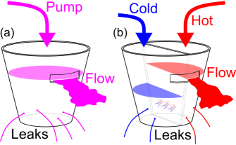
Figure 1: (Color online) Bucket model for (a) a conventional laser and (b) a spin laser.Lee2012:PRB Water added to the bucket represents the carriers, and the water coming out represents the emitted light. Small leaks depict spontaneous emission, and overflowing water reaching the large opening corresponds to the lasing threshold. In (b) the two halves represent two spin populations (hot and cold water in the analogy), and they are filled separately. The partition between them is not perfect: spin relaxation can cause the two populations to mix. The color code indicates conservation of angular momentum; an unpolarized pumping (violet) is an equal mixture of two polarized contributions (red and blue).

An intuitive picture for a spin laser is provided by a bucket model in Fig. 1.Lee2012:PRB ; Zutic2014:NN The uneven water levels represent the spin imbalance in the laser, which implies the following: (i) Lasing threshold reduction - in a partitioned bucket, less water needs to be pumped for it to overfill. There are also two thresholds (for cold and hot water).Gothgen2008:APL (ii) Gain asymmetry - an unequal amount of hot and cold water comes out. A small spin imbalance of pumped carriers can (the two water levels slightly above and below the opening, respectively) result in a complete imbalance in the polarization of the emitted light (here only hot water gushes out) and, consequently, spin-filtering. These effects are attained at room temperature with either optical or electrical injection. The latter experimental demonstrationCheng2014:NN is a breakthrough towards practical use of spin lasers.

Perhaps the most promising opportunity to overcome the limitations of conventional lasers lies in the dynamic operation of spin lasers, predicted to provide enhanced modulation bandwidth, improved switching properties, and reduced parasitic frequency modulation, i. e., chirp.Lee2014:APL ; Lee2012:PRB ; Lee2010:APL ; Boeris2012:APL Moreover, experiments have confirmed that in a given device a characteristic frequency of polarization oscillations of the emitted light can significantly exceed the corresponding frequency of the intensity oscillations.Jahme2010:APL ; Gerhardt2011:APL ; Hopfner2014:APL This behavior was attributed to birefringence - an anisotropy of the index of refraction, considered detrimental in conventional lasers.Chuang:2009

What should we then require to attain high-frequency operation in spin lasers? Can we provide guidance for the design of an active region and a choice of the resonant cavity? Unfortunately, to address similar questions, we cannot simply rely on the widely used rate-equation description of spin lasers,Rudolph2003:APL ; Holub2007:PRL ; Lee2012:PRB ; SanMiguel1995:PRA ; Gahl1999:IEEEJQE but instead we need to formulate a microscopic description. The crucial consideration is detailed knowledge of the spectral (energy-resolved) optical gain obtained from an accurate description of the electronic structure in the active region, already important to elucidate a steady-state operation of a spin laser.

A typical vertical geometry, the so-called vertical cavity surface emitting lasers (VCSELs),Chuang:2009 ; Coldren:2012 ; Fu:2003 ; Michalzik:2013 used in nearly all spin lasers, is illustrated in Fig. 2(a). Even among conventional lasers, VCSELs are recognized for their unique properties, making them particularly suitable for optical data transmission.Michalzik:2013 The resonant cavity is usually in the range of the emission wavelength, providing a longitudinal single-mode operation. It is formed by a pair of parallel highly reflective mirrors made of distributed Bragg reflectors (DBRs), a layered structure with varying refractive index. The gain active (gain) region, usually consists of III-V quantum wells (QWs) or quantum dots (QDs).Basu2008:APL ; Basu2009:PRL ; Saha2010:PRB ; Oszwaldowski2010:PRB ; Lee2012:PRB ; Adams2012:IEEEPJ ; Khaetskii2013:PRL

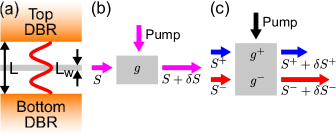
Figure 2: (a) (Color online) Geometry of a vertical cavity surface-emitting laser. The resonant cavity of length $L$ is formed between the two mirrors made of distributed Bragg reflectors (DBRs). The shaded region represents the active (gain) region of length $L_{W}$. The profile of a longitudinal optical mode is sketched. Schematic of the optical gain, $g$, in the active region for a conventional laser (b) and a spin laser (c). With external pumping/injection, a photon density $S$ increases by $\delta S$ as it passes across the gain region.note_expgain In the spin laser, this increase depends on the positive ($+$)/negative($-$) helicity of the light, $S=S^{+}+S^{-}$.

The key effect of the active region is producing a stimulated emission and coherent light that makes the laser such a unique light source. The corresponding optical gain that describes stimulated emission, under sufficiently strong pumping/injection of carriers, can be illustrated pictorially in Figs. 2(b) and  2(c) for both conventional and spin lasers, respectively. In the latter case, it is convenient to decompose the photon density into different circular polarizations and distinguish that the gain is generally polarization-dependent. If we neglect any losses in the resonant cavity, such a gain would provide an exponential growth rate with the distance across a small segment of gain material.Coldren:2012 Since both static and dynamic operations of spin lasers depend crucially on their corresponding optical gain, our focus will be to provide its microscopic description derived from an accurate electronic structure of an active region.

After this Introduction, in Sec. II we provide a theoretical framework to calculate the gain in quantum well-based lasers. In Sec. III, we describe the corresponding electronic structure and the carrier populations under spin injection, the key prerequisites to understanding the spin-dependent gain and its spectral dependence, discussed in Sec. IV. Our gain calculations in Sec. V explain how the steady-state properties of spin lasers can be modified by spin-polarized carriers, carrier density, and resonant cavity design. In Sec. VI, we analyze the influence of a uniaxial strain in the active region, which introduces a large birefringence with the resulting oscillation frequency that would significantly exceed the frequency range possible in conventional lasers. In Sec. VII, we describe various considerations for the optimized design of spin lasers and the prospect of their ultrahigh-frequency operation. A brief summary in Sec. VIII ends our paper.

II Theoretical framework

While both QWs and QDs,Basu2008:APL ; Basu2009:PRL ; Saha2010:PRB are used for the active region of spin lasers, we focus here on the QW implementation also found in most of the commercial VCSELs.Michalzik:2013 To obtain an accurate electronic structure in the active region, needed to calculate optical gain, we use the $8\times 8$ $\bm{k{\cdot}p}$ $\bm{k{\cdot}p}$ method.Holub2011:PRB The total Hamiltonian of the QW system, with the growth axis along the $z$ direction, is

$$H_{\textrm{QW}}(z)=H_{kp}(z)+H_{\textrm{st}}(z)+H_{\textrm{O}}(z),$$ (1)

where $H_{kp}(z)$ denotes the $\bm{k{\cdot}p}$ term, $H_{\textrm{st}}(z)$ describes the strain term, and $H_{\textrm{O}}(z)$ includes the band-offset at the interface that generates the QW energy profile. The explicit form of these different terms for zinc-blende crystals is given in Appendix A.

Because common nonmagnetic semiconductors are well characterized by the vacuum permeability, $\mu_{0}$, a complex dielectric function $\varepsilon(\omega)=\varepsilon_{r}(\omega)+\varepsilon_{i}(\omega)$, where $\omega$ is the photon (angular) frequency, can be used to simply express the dispersion and absorption of electromagnetic waves. The absorption coefficient describing gain or loss of the amplitude of an electromagnetic wave propagating in such a medium is the negative value of the gain coefficient (or gain spectrum),Haug:2004 ; Chuang:2009 ; note_gain

$$g^{a}(\omega)=-\frac{\omega}{cn_{r}}\epsilon^{a}_{i}(\omega)\,,$$ (2)

where $c$ is the speed of light, $n_{r}$ is the dominant real part of the refractive index of the material,Haug:2004 and $\varepsilon^{a}_{i}(\omega)$ is the imaginary part of the dielectric function which generally depends on the polarization of light, $a$, given by

$$\varepsilon^{a}_{i}(\omega)=C_{0}\underset{c,v,\vec{k}}{\sum}\left|p^{a}_{cv\vec{k}}\right|^{2}\left(f_{v\vec{k}}-f_{c\vec{k}}\right)\delta\left[\hbar\omega_{{cv}\vec{k}}-\hbar\omega\right],$$ (3)

where the indices $c$ (not to be confused with the speed of light) and $v$ label the conduction and valence subbands, respectively, $\vec{k}$ is the wave vector, $p^{a}_{cv\vec{k}}$ is the interband dipole transition amplitude, $f_{c(v)\vec{k}}$ is the Fermi-Dirac distribution for the electron occupancy in the conduction (valence) subbands, $\hbar$ is the Planck’s constant, $\omega_{{cv}\vec{k}}$ is the interband transition frequency, and $\delta$ is the Dirac delta-function, which is often replaced to include broadening effects for finite lifetimes.Chuang:2009 ; Chow:1999 The constant $C_{0}$ is $C_{0}=4\pi^{2}e^{2}/(\varepsilon_{0}m_{0}^{2}\omega^{2}\Omega)$, where $e$ is the electron charge, $m_{0}$ is the free electron mass, and $\Omega$ is the QW volume.

Analogously to expressing the total photon density in Fig. 2, as the sum of different circular polarizations, $S=S^{+}+S^{-}$, in spin-resolved quantities we use subscripts to describe different spin projections, i. e., eigenvalues of the $\sigma_{z}$ Pauli matrix. The total electron/hole density can be written as the sum of the spin up ($+$) and the spin down ($-$) electron/hole densities, $n=n_{+}+n_{-}$ and $p=p_{+}+p_{-}$. In this convention,Gothgen2008:APL ; Lee2010:APL ; Lee2014:APL using the conservation of angular momentum between carriers and photons, the recombination terms are $n_{+}p_{+}$, $n_{-}p_{-}$, while the corresponding polarization of the emitted light depends on the character of the valence band holes.note_rate_holes We can simply define the carrier spin polarization

$$P_{\alpha}=(\alpha_{+}-\alpha_{-})/(\alpha_{+}+\alpha_{-}),$$ (4)

where $\alpha=n$, $p$.note_polarizations

Using the dipole selection rules for the spin-conserving interband transitions, the gain spectrum,

$$g^{a}(\omega)=g^{a}_{+}(\omega)+g^{a}_{-}(\omega)$$ (5)

can be expressed in terms of the contributions of spin up and down carriers. To obtain $g^{a}_{+(-)}(\omega)$, the summation of conduction and valence subbands is restricted to only one spin: $\underset{c}{\sum}\rightarrow\underset{c+(-)}{\sum}$ and $\underset{v}{\sum}\rightarrow\underset{v+(-)}{\sum}$ in Eq. (3).

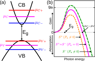
Figure 3: (Color online) (a) Energy band diagram with a bandgap $E_{g}$ and chemical potentials in conduction (valence) bands, $\mu_{C}$ ($\mu_{V}$) that in the presence of spin-polarized carriers become spin-dependent: $\mu_{C(V)+}\neq\mu_{C(V)-}$. Unlike the rest of our analysis, here holes are spin-polarized. (b) Gain spectrum for unpolarized (solid) and spin-polarized electrons (dashed curves). Positive gain corresponds to the emission and negative gain to the absorption of photons. The gain threshold $g_{th}$, required for lasing operation, is attained only for $S^{-}$ helicity of light.

To see how spin-polarized carriers could influence the gain, we show chemical potentials, $\mu_{C(V)}$, for a simplified conduction (valence) band in Fig. 3(a). The spin imbalance in the active region implies that $\mu_{C(V)}$ will also become spin-dependent. Such different chemical potentials lead to the dependence of gain on the polarization of light, described in Fig. 3(b). Without spin-polarized carriers, the gain is the same for $S^{+}$ and $S^{-}$ helicity of light. In an ideal semiconductor laser, $g>0$ requires a population inversion for photon energies, $E_{g}<\hbar\omega<(\mu_{C}-\mu_{V})$. However, a gain broadening is inherent to lasers and, as depicted in Fig. 3(b), $g>0$ even below the bandgap, $\hbar\omega<E_{g}$. If we assume $P_{n}\neq 0$ [recall Eq. (4)] and $P_{p}=0$ (accurately satisfied, as spins of holes relax much faster than electrons), we see different gain curves for $S^{+}$ and $S^{-}$. The crossover from emission to absorption is now in the range of ($\mu_{C-}-\mu_{V-}$) and ($\mu_{C+}-\mu_{V+}$).

Optical injection of spin-polarized electrons is the most frequently used method to introduce spin-imbalance in lasers. Some spin lasers are therefore readily available since they can be based on commercial semiconductor lasers to which a source of circularly polarized light is added subsequently.Rudolph2003:APL Such spin injection can be readily understood from dipole optical selection rules which apply for both excitation and radiative recombination.Meier:1984 ; Zutic2004:RMP

A simplified band diagram for a zinc-blende QW semiconductor with the corresponding interband transitions is depicted in Fig. 4. At the Brillouin zone center, the valence band degeneracy of heavy and light holes (HH, LH) in the bulk semiconductor is lifted for QWs due to quantum confinement along the growth direction. The angular momentum of absorbed circularly polarized light is transferred to the semiconductor. Electrons’ orbital momenta are directly oriented by light and, through spin-orbit interaction, their spins become polarized.Meier:1984 While initially holes are also polarized, their spin polarization is quickly lost.Zutic2004:RMP Thus, as in Fig. 3(b), we assume throughout this work $P_{p}=0$, unless stated otherwise.

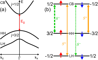
Figure 4: (Color online) Schematic band structure and optical selection rules in zinc-blende QWs. (a) Conduction band (CB) and valence band with heavy and light holes (HH, LH) labeled by their total angular momentum $j=1/2$ and $j=3/2$, representing the states of the orbital angular momentum $l=0$ and $1$, respectively (Appendix A). (b) Interband dipole transitions near the band edge of a QW for light with positive and negative helicity, $S^{\pm}$, between the sublevels labeled by $m_{j}$, the projection of the total angular momentum on the $+z$-axis (along the growth direction). The small arrows represent the projection of spin 1/2 of the orbital part that contributes to the transition, indicating that dipole transitions do not change spin (Appendix B).

The spin polarization of excited electrons depends on the photon energy for $S^{+}$ or $S^{-}$ light. From Fig. 4(b) we can infer that if only CB-HH are involved, $|P_{n}|\rightarrow 1$. At a larger $\hbar\omega$, involving also CB-LH transitions, $|P_{n}|$ is reduced. Expressing $S^{\pm}\propto Y_{1}^{\pm 1}$, where $Y_{l}^{m}$ is the spherical harmonic, provides a simple connection between dipole selection rules and the conservation of angular momentum in optical transitions (Appendix B).

III Electronic structure

For our microscopic description of spin lasers we focus, on a (Al,Ga)As/GaAs-based active region, a choice similar to many commercial VCSELs. We consider an $\textrm{Al}_{0.3}\textrm{Ga}_{0.7}\textrm{As}$ barrier and a single 8 nm thick GaAs QW.note_parameters The corresponding electronic structure of both the band dispersion and the density of states (DOS) is shown in Fig. 5. Our calculations, based on the $\bm{k{\cdot}p}$ method and the 8$\times$8 Hamiltonian from Eq. (1) (Appendix A), yield two confined CB subbands: CB1, CB2, and five VB subbands, labeled in Fig. 5(a) by the dominant component of the total envelope function at $\vec{k}=0$. The larger number of confined VB subbands stems from larger effective masses for holes than electrons.GaAs_masses These differences in the effective masses also appear in the DOS shown in in Fig. 5(b).

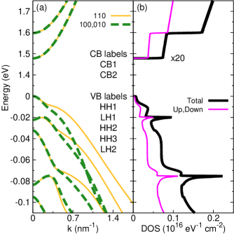
Figure 5: (Color online) (a) Band structure for the $\textrm{Al}_{0.3}\textrm{Ga}_{0.7}\textrm{As}$/GaAs QW for different $k$-directions along [100], [010], and [110]. (b) DOS calculated from (a). The conduction band DOS is multiplied by a factor of 20 to match the valence band scale. The bandgap is $E_{g}=1.479\;\textrm{eV}$ (CB1-HH1 energy difference).

As we seek to describe the gain spectrum in the active region, once we have the electronic structure, it is important to understand the effects associated with carrier occupancies though injection/pumping [recall Fig. 2, Eqs. (2) and (3)]. In Figs. 6 (a), (c), and (e) we show both examples of injected unpolarized ($P_{n}=0$) and spin-polarized ($P_{n}=0.5$) electrons as seen in the equal and spin-split CB chemical potentials, respectively. The carrier populationColdren:2012 is given in Figs. 6(b), (d), and (f) using the product of the Fermi-Dirac distribution and the DOS for CB and VB for both spin projections.

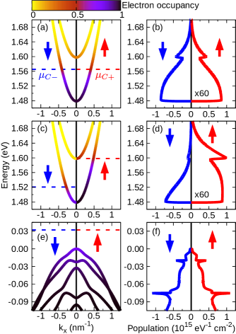
Figure 6: (Color online) Band structure of Fig. 5(a) with electron occupancy for (a) $P_{n}$=0, (c) $P_{n}=0.5$, and (e) $P_{p}=0$. Carrier population expressed as a product of DOS from Fig. 5(b) and the Fermi-Dirac distribution of electrons for (b) $P_{n}$=0, (d) $P_{n}=0.5$, and (f) $P_{p}=0$. The carrier density is fixed at $n=p=3\times 10^{12}\;\textrm{cm}^{-2}$ and $T=300\;\textrm{K}$. The negative (positive) side of the x-axis represents spin down (up) electrons, dashed lines denote chemical potentials. The CB population is multiplied by 60 and shown in the same scale as for the VB.

IV Understanding the spin-dependent gain

From the conservation of angular momentum and polarization-dependent optical transitions, we can understand that even in conventional lasers, carrier spin plays a role in determining the gain. However, in the absence of spin-polarized carriersnote_nonmagnetic the gain is identical for the two helicities: $g^{+}=g^{-}$, and we recover a simple description (spin- and polarization-independent) from Fig. 2(b). In our notation, $g^{\pm}_{\pm}$, the upper (lower) index refers to the circular polarization (carrier spin) [recall Eq. (5)].

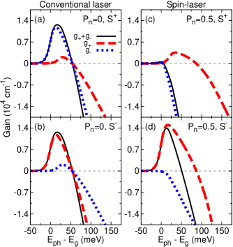
Figure 7: (Color online) Gain spectra shown as a function of photon energy measured with respect to the energy bandgap. Conventional laser, $P_{n}=0$ for (a) $S^{+}$ and (b) $S^{-}$ light polarization. spin lasers, $P_{n}=0.5$ for (c) $S^{+}$ and (d) $S^{-}$ light polarizations. The carrier density $n=p=3\times 10^{12}\;\textrm{cm}^{-2}$ and $T=300\;\textrm{K}$ are the same as in Fig. 6.

This behavior can be further understood from the gain spectrum in Figs. 7(a) and (b), where we recognize that $g^{+}=g^{-}$ requires: (i) $g^{+}_{-}=g^{-}_{+}$ and $g^{+}_{+}=g^{-}_{-}$, dominated by CB1-HH1 ($1.479\;\textrm{eV}=E_{g}$) and CB1-LH1 ($1.501\;\textrm{eV}$) transitions, respectively (recall Fig. 5). No spin-imbalance implies spin-independent $\mu_{C}$ and $\mu_{V}$ [Fig. 3(a)] and thus $g^{\pm}$, $g^{\pm}_{+}$, and $g^{\pm}_{-}$, all vanish the photon energy E${}_{\textrm{ph}}=\hbar\omega=\mu_{C}-\mu_{V}$. Throughout our calculations we choose a suitable $\cosh^{-1}$ broadeningChow:1999 with a full width at half-maximum (FWHM) of $19.75\;\textrm{meV}$, which accurately recovers the gain of conventional (Al,Ga)As/GaAs QW systems.

We next turn to the gain spectrum of spin lasers. Why is their output different for $S^{+}$ and $S^{-}$ light, as depicted in Fig. 2(b)? Changing only $P_{n}=0.5$ from Figs. 7(a) and (b), we see very different results for $S^{+}$ and $S^{-}$ light in Figs. 7(c) and (d). $P_{n}>0$ implies that $\mu_{C+}>\mu_{C-}$ [see Fig. 6(c)], leading to a larger recombination between the spin up carriers ($n_{+}p_{+}>n_{-}p_{-}$) and thus to a larger $g_{+}$ for $S^{+}$ and $S^{-}$ (red/dashed line) than $g_{-}$ (blue/dashed line). The combined effect of having spin-polarized carriers and different polarization-dependent optical transitions for spin up and down recombination is then responsible for $g^{+}\neq g^{-}$, given by solid lines in Figs. 7(c) and 7(d). For this case, the emitted light $S^{-}$ exceeds that with the opposite helicity, $S^{+}$, and there is a gain asymmetry, Holub2007:PRL ; Hovel2008:APL ; Basu2009:PRL another consequence of the polarization-dependent gain. The zero gain is attained at $\mu_{C+}-\mu_{V}$ for spin up (red curves) and $\mu_{C-}-\mu_{V}$ for spin down transitions (blue curves). The total gain, including both of these contributions, reaches zero at an intermediate value. Without any changes to the band structure, a simple reversal of the carrier spin-polarization, $P_{n}\rightarrow-P_{n}$, reverses the role of preferential light polarization.

V Steady-state gain properties

Within our framework, providing a spectral information for the gain, we can investigate how the carrier density and its spin polarization, which can be readily modified experimentally, can change the steady-state operation of spin lasers. Specific to VCSELs, it is important to examine how their laser operation is related to the choice of a resonant cavity which defines the photon energy at which the constructive interference takes place.

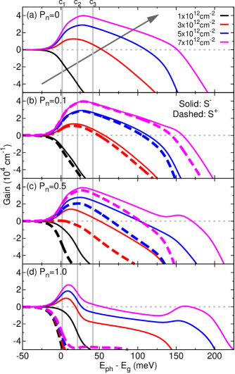
Figure 8: (Color online) Evolution of the gain spectra with carrier density for: (a) $P_{n}=0$, (b) $P_{n}=0.1$, (c) $P_{n}=0.5$, and (d) $P_{n}=1.0$. In order to achieve emission, a certain value of carrier density should be added to the system. The second peak at $\textrm{E}_{\textrm{ph}}-\textrm{E}_{\textrm{g}}\sim 150\;\textrm{meV}$ is related to transitions of CB2-HH2. Transitions of CB2-LH2 at $\textrm{E}_{\textrm{ph}}-\textrm{E}_{\textrm{g}}\sim 200\;\textrm{meV}$ can be seen in the broader second peak for $P_{n}=1.0$. The difference between $g^{+}$ and $g^{-}$ that arise due to spin-polarized carriers in the system increases with $P_{n}$. For $P_{n}=1.0$ there is no emission of $S^{+}$ polarized light, i. e., this component is totally absorbed by the system. The diagonal arrow in Fig. 8 indicates the increase of carrier density in the curves.

Most of the QW-based lasers do not have a doped active region, and they rely on a charge neutral carrier injection (electrical or optical).Coldren:2012 Here we choose $n=p=1,3,5,7\times 10^{12}\;\textrm{cm}^{-2}$, and spin polarizations $P_{n}=0,0.1,0.5,1$, respectively. Electrical injection in intrinsic III-V QWs using Fe or FeCo allows for $|P_{n}|\sim 0.3-0.7$,Hanbicki2002:APL ; Zega2006:PRL ; Salis2005:APL while $|P_{n}|\rightarrow 1$ is attainable optically at room temperature.Zutic2004:RMP In most of the spin lasers, $|P_{n}|\lesssim 0.2$ in the active region. We focus on three resonant cavity positions: $\textrm{c}_{1}$, $\textrm{c}_{2}$, $\textrm{c}_{3}$ (vertical lines), defining the corresponding energy of emitted photons $\textrm{c}_{1}=1.48\;\textrm{eV}\sim 1.479$ eV (CB1-HH1 transition), $\textrm{c}_{2}=1.5\;\textrm{eV}\sim 1.501$ eV (CB1-LH1 transition), and $\textrm{c}_{3}=1.52\;\textrm{eV}$ (at the high energy side of the gain spectrum).

The corresponding results are given in Fig. 8 showing gain spectra different for $S^{+}$ and $S^{-}$. This gain asymmetry, $g^{+}\neq g^{-}$, is more pronounced at larger $P_{n}$; at $P_{n}=1$, there is even no $S^{+}$ emission. While this trend is expected and could be intuitively understood, there is a more complicated dependence of the gain asymmetry, $g^{-}(\hbar\omega)-g^{+}(\hbar\omega)$ on the carrier density and the choice of the detuning,Haug:2004 the energy (frequency) difference between the gain peak and the resonant cavity position.

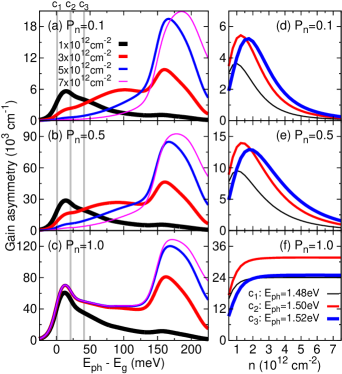
Figure 9: (Color online) Gain asymmetry obtained from Fig. 8 for: (a) $P_{n}=0.1$, (b) $P_{n}=0.5$, and (c) $P_{n}=1.0$. As more carriers are added to the system, the asymmetry peak shifts to higher energies, however, this energy region is not necessarily in the regime of a positive gain. Gain asymmetry as a function of carrier density for: (d) $P_{n}=0.1$, (e) $P_{n}=0.5$, and (f) $P_{n}=1.0$. Similar to the case of Figs. 9(a)-(c), the asymmetry peaks may not correspond to positive gain.

The gain asymmetry is one of the key figures of merit for spin lasers, and it can be viewed as crucial for their spin-selective properties, including robust spin-filtering or spin-amplification, in which even a small $P_{n}$ (few percent) in the active region leads to an almost complete polarization of the emitted light (of just one helicity).Iba2011:APL Unfortunately, how to enhance the gain asymmetry, beyond just increasing $P_{n}$, is largely unexplored.

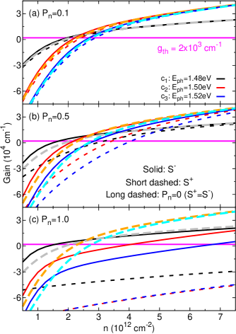
Figure 10: (Color online) Gain as a function of carrier density for: (a) $P_{n}=0.1$, (b) $P_{n}=0.5$, and (c) $P_{n}=1.0$, with the cavity choices $\textrm{c}_{1}$, $\textrm{c}_{2}$, and $\textrm{c}_{3}$. Comparing: (i) solid and short-dashed lines we can examine the spin-filtering effect, and (ii) solid and long-dashed curves, we can examine the threshold reduction. The solid horizontal line indicates the gain threshold, i.e., the losses in the cavity. To achieve the lasing, the value of gain must be greater than the gain threshold.

To establish a more systematic understanding of a gain asymmetry, we closely examine $g^{-}(\hbar\omega)-g^{+}(\hbar\omega)$ in Figs. 9(a)-9(c) for different $P_{n}$, carrier densities, and resonant cavities. Increasing $n$, the anisotropy peak shifts to higher $\hbar\omega$, indicating an occupation of higher energy subbands. However, the absolute anisotropy peak is not always in the emission region. For a desirable operation of a spin laser we should seek a large gain anisotropy with a positive (and a preferably large) gain. Complementary information is given by Figs. 9(d)-9(f) with a density evolution of $g^{-}-g^{+}$ for different cavity positions and $P_{n}$. Again, we see that the gain asymmetry peak can be attained outside of the lasing region.

The results in Fig. 9 have shown a complex evolution of the gain asymmetry with the cavity position and carrier density. We now repeat a similar analysis for the gain itself in Fig. 10. The gain calculated for two helicities and unpolarized light ($S^{+}=S^{-}$), provides a useful guidance for the threshold reduction and the spin-filtering effect, invoked in a simple bucket model from Fig. 1.

We first consider $P_{n}=0.1$ which shows a behavior with an increase in $n$ or, equivalently, an increase in injection, that could be expected from the bucket model. The threshold value of the gain (the onset of an overflowing bucket), $g_{\textrm{th}}$, is first reached for $S^{-}$, then for unpolarized light, a sign of threshold reduction, and finally for $S^{+}$ (a subdominant helicity from the conservation of angular momentum and $P_{n}>0$). Therefore there is a spin-filtering interval of $n$ (small, since $P_{n}$ itself is small) where we expect lasing with only one helicity. A similar behavior appears for all the cavity choices $\textrm{c}_{1}$, $\textrm{c}_{2}$, and $\textrm{c}_{3}$.

We next turn to $P_{n}=0.5$ where $\textrm{c}_{1}$ shows trends expected both from the bucket model and early work on spin lasers.Rudolph2003:APL ; Holub2007:PRL An increase from $P_{n}=0.1$ to $0.5$ enhances the threshold reduction and the spin-filtering interval. However, different cavity positions $\textrm{c}_{2}$ and $\textrm{c}_{3}$ reveal a different behavior. There is a region where unpolarized light $S^{+}=S^{-}$ (long dashed lines) yields a greater gain than for $S^{-}$ (solid lines). For $\textrm{c}_{3}$ the threshold is attained at smaller $n$ for unpolarized light than for negative helicity, i.e., there is no threshold reduction.note_Holub With $P_{n}=1.0$, the threshold reduction is only possible for $\textrm{c}_{1}$.

These results reinforce the possibility for a versatile spin-VCSEL design by a careful choice of the resonant cavity, but they also caution that, depending on the given resonant cavity, the usual intuition about the influence of carrier density and spin polarization on the laser operation may not be appropriate.

VI Strain-induced birefringence

An important implication of an anisotropic dielectric function is the phenomenon of birefringence in which the refractive index, and thus the phase velocity of light, depends on the polarization of light.Coldren:2012 Due to phase anisotropies in the laser cavity,note_phase the emitted frequencies of linearly polarized light in the x- and y-directions ($S^{x}$ and $S^{y}$) are usually different. Such birefringence is often undesired for the operation of conventional lasers since it is the origin for the typical complex polarization dynamics and chaotic polarization switching behavior in VCSELs.vanExter1997:PRB ; SanMiguel1995:PRA ; Sondermann2004:IEEE ; Al-Seyab2011:IEEEPJ ; Virte2013:NP While strong values of birefringence are usually considered to be an obstacle for the polarization control in spin-polarized lasers,Hovel2008:APL ; Frougier2015:OE the combination of a spin-induced gain asymmetry with birefringence in spin-VCSELs allows us to generate fast and controllable oscillations between $S^{+}$ and $S^{-}$ polarizations.Gerhardt2011:APL ; Hopfner2014:APL The frequency of these polarization oscillations is determined by the linear birefringence in the VCSEL cavity, and it can be much higher than the frequency of relaxation oscillations of the carrier-photon system in conventional VCSELs. This may pave the way towards ultrahigh bandwidth operation for optical communications.Gerhardt2011:APL ; Gerhardt2012:AOT ; Lee2014:APL

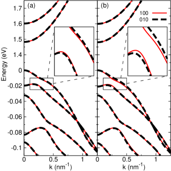
Figure 11: (Color online) Band structure with uniaxial strain in the active region for (a) $\varepsilon_{xx}\sim 0.019\%$ and (b) $\varepsilon_{xx}\sim 0.058\%$. The inset shows a zoom around the HH1 and LH1 interaction region, where the difference between [100] and [010] directions is more visible. The energy gap of the system is $E_{g}\sim 1.483\;\textrm{eV}$ for case (a) and $E_{g}\sim 1.481\;\textrm{eV}$ for case (b).

In order to investigate birefringence effects in the active region of a conventional laser, we consider uniaxial strain by extending the lattice constant in x-direction. For simplicity, we assume the barrier to have the same lattice constant as GaAs, $5.6533\;\textrm{\AA}$, in y-direction. Therefore, both barrier and well regions will have the same extension in x-direction. For $a_{x}=5.6544\;\textrm{\AA}$ we have the corresponding element of the strain tensor $\varepsilon_{xx}\sim 0.019\%$, while $a_{x}=5.6566\;\textrm{\AA}$ gives $\varepsilon_{xx}\sim 0.058\%$.

The effect of uniaxial strain in the band structure is presented in Fig. 11(a) and (b) for $\varepsilon_{xx}\sim 0.019\%$ and $\varepsilon_{xx}\sim 0.058\%$, respectively. The labeling and ordering of subbands follows the same as that in Fig. 5(a). Just this slight anisotropy in the x- and y-lattice constants creates a difference in subbands for the [100] and [010] directions. In the inset we show the region around the anti-crossing of HH1 and LH1 subbands, where the difference is more visible.

In addition to the differences induced in the band structure, the uniaxial strain also induces a change in the dipole selection rules between $S^{x}$ and $S^{y}$ light polarizations, which can be seen in the gain spectra we present in Fig. 12(a) and 12(b) for $\varepsilon_{xx}\sim 0.019\%$ and $\varepsilon_{xx}\sim 0.058\%$, respectively. Reflecting the features of the band structure, we notice for the emission region of the gain spectra that the largest difference between $g^{x}$ and $g^{y}$ is around the HH1 and LH1 energy regions (between $\textrm{c}_{1}$ and $\textrm{c}_{3}$ cavity positions, approximately). In the absorption regime (negative gain) we notice $g^{x}<g^{y}$, while in the emission regime (positive gain) we have $g^{x}>g^{y}$. This feature is more visible in Fig. 12(b).

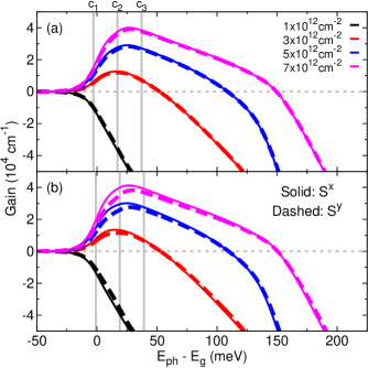
Figure 12: (Color online) Uniaxial strain modification of gain spectra for strain (a) $\varepsilon_{xx}\sim 0.019\%$ and (b) $\varepsilon_{xx}\sim 0.058\%$. The anisotropy in the lattice constants for x- and y-directions modifies the output light polarization of the laser. Since there are no spin-polarized carriers in the system, $g^{+}=g^{-}$.

To calculate the birefringence coefficient in the active region, we used the definition of Ref. Mulet2002:IEEEJQE, , given by

$$\gamma_{p}(\omega)=-\frac{\omega}{2n_{e}n_{g}}\delta\varepsilon_{r}(\omega)\;,$$ (6)

where $\omega$ is the frequency of the longitudinal mode in the cavity, $n_{e}$ is the effective index of refraction of the cavity, and $n_{g}$ is the group refractive index. For simplicity, we assume $n_{e}=n_{g}$. The real part of the dielectric function can be obtained from the imaginary part using the Kramers-Kronig relations.Haug:2004

We present the birefringence coefficient in Fig. 13(a) and 13(b) for $\varepsilon_{xx}\sim 0.019\%$ and $\varepsilon_{xx}\sim 0.058\%$, respectively. We notice that this strain in the active region, responsible for modest changes in the gain spectra, produces birefringence values of the order of $10^{11-12}$ Hz which may be exploited to generate fast polarization oscillations. Furthermore, when increasing the strain amount by $\sim 0.04\%$ from case (a) to case (b), the value of $\gamma_{p}$ increases approximately threefold.JansenvanDoorn1998:IEEEJQE We also included in our calculations spin-polarized electrons and notice that they have only a small influence in the birefringence coefficient. Although they change $|g^{x}|$ and $|g^{y}|$ slightly , the asymmetry is not affected at all for small spin polarizations of 10-20%, which are relevant values in real devices.

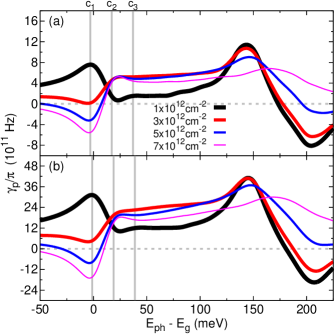
Figure 13: (Color online) Birefringence coefficient as a function of photon energy considering (a) $\varepsilon_{xx}\sim 0.019\%$ and (b) $\varepsilon_{xx}\sim 0.058\%$. Just an increase of $0.0022\;\textrm{\AA}$ in $a_{x}$ increases $\gamma_{p}$ by approximately 3 times. The two peaks, around $\textrm{E}_{\textrm{ph}}-\textrm{E}_{\textrm{g}}\sim 0$ meV and $\textrm{E}_{\textrm{ph}}-\textrm{E}_{\textrm{g}}\sim 150$ meV are related to transitions from CB1 and CB2. Transitions related to CB2 are in the absorption regime, not visible in Fig. 12.

Investigating the effect of different cavity designs, we present the values of $\gamma_{p}$ in Figs. 14(a) and 14(b) for $\varepsilon_{xx}\sim 0.019\%$ and $\varepsilon_{xx}\sim 0.058\%$, respectively. We chose the same photon energies as for the case without birefringence assuming that the different values for the strain-induced birefringence in the active region will not significantly affect the cavity resonance for reasons of simplicity. For the two different strain types the behavior of $\gamma_{p}$ is very similar for the same resonance energy. Comparing different cavity designs we observe that for $\textrm{c}_{1}$, the value of $\gamma_{p}$ strongly decreases and also changes sign with the carrier density, $n$. In contrast, for $\textrm{c}_{2}$ and $\textrm{c}_{3}$, $\gamma_{p}$ is always positive. After a slow increase with $n$, $\gamma_{p}$ becomes flat, and nearly independent of the carrier density.

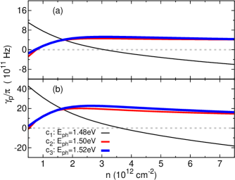
Figure 14: (Color online) Birefringence coefficient as function of the carrier density for (a) $\varepsilon_{xx}\sim 0.019\%$ and (b) $\varepsilon_{xx}\sim 0.058\%$. For different cavity designs the behavior of $\gamma_{p}$ can be completely different. The carrier density values where $\gamma_{p}$ changes sign in cavity $\textrm{c}_{1}$ and the flat region in cavities $\textrm{c}_{2}$ and $\textrm{c}_{3}$ are already in the lasing regime.

For consistency, we have also calculated the DBR contributions using the approach given by Mulet and Balle.Mulet2002:IEEEJQE For large anisotropies in the DBR, the birefringence coefficient is on the order of $10^{10}$ Hz, consistent with the measurements given by van Exter et al.vanExter1997:PRB Therefore, for the investigated strain conditions, the main contribution to $\gamma_{p}$ comes from the active region and it is a very versatile parameter that can be fine-tuned using both carrier density and cavity designs, possibly even changing its sign and reaching carrier density-independent regions.

VII Ultra high-frequency operation

Lasers could provide the next generation of parallel optical interconnects and optical information processing.Fu:2003 ; Coldren:2012 ; Michalzik:2013 ; Kaminow:2013 ; Agrawal:2002 ; Ciftcioglu2012:OE ; Miller2009:PIEEE The growth in communicationHilbert2011:S and massive data centersreport:2012 will pose further limitations on interconnects.itrs:2011 Conventional metallic interconnects used in multicore microprocessors are increasingly recognized as the bottleneck in maintaining Moore’s law scaling and the main source of power dissipation.Miller2009:PIEEE ; itrs:2011 Optical interconnects can effectively address the related limitations, such as the electromagnetic crosstalk and signal distortion, while providing a much larger bandwidth.Ciftcioglu2012:OE ; Miller2009:PIEEE VCSELs are considered particularly suitable for short-haul communication and on-chip interconnects.Michalzik:2013 However, to fully utilize their potential, it would be important to explore the paths for their high-frequency operation and achieve a higher modulation bandwidth, limited for conventional lasers to about $\sim 50$ GHz.Michalzik:2013 ; Westbergh2013:EL

How can we understand the frequency limitation of a laser? Why would a higher frequency modulation lead to a decrease in a signal-to-noise ratio and limit the effective bandwidth? An accurate analogy is provided by a driven and damped harmonic oscillator. The laser response, just like the harmonic oscillator, is unable to follow a high enough modulation frequency. A Lorenzian-like frequency-dependent displacement of a harmonic oscillator closely matches a modulation response of a laser, decreasing as $1/\omega$, above the corresponding resonance frequency, known as the relaxation oscillation frequency, $\omega_{R}$, representing a natural oscillation between the carriers and photons and often used to estimate the bandwidth of a laser.Coldren:2012 ; Michalzik:2013 ; Kapon:1999

To realize a high-speed operation in conventional lasers requires a careful design and optimization of many parameters. Attaining a high $\omega_{R}$ is closely related to optimizing the gain which increases with $n$,note_dope but decreases with photon density $S$, known as the gain compressionnote_compress which would be desirable to minimize. For a small-signal modulation $S(t)=S_{0}+\delta S(t)$, above the threshold,Coldren:2012

$$\omega^{2}_{R}\approx v_{g}(dg/dn)S_{0}/\tau_{\textrm{ph}},$$ (7)

where $v_{g}$ is the group velocity of the relevant mode, $dg/dn$ is the differential gain at the threshold, and $\tau_{\textrm{ph}}$ is the photon lifetime. While $\omega_{R}$ increases with $S_{0}$, a larger $S_{0}$, through gain compression, is detrimental by diminishing the differential gain. There are additional factors, beyond Eq. (7), required for a high $\omega_{R}$, such as minimizing the transport time for carriers to reach the active region, achieving a high carrier escape rate into the QW barriers, and minimizing extrinsic parasitic effects between the intrinsic laser and the driving circuit.Michalzik:2013 ; Kapon:1999

Introducing spin-polarized carriers offers additional possibilities to enhance $\omega_{R}$, corresponding to the modulation of the emitted $S$, beyond the frequencies attainable in conventional lasers. In the regime of small-signal modulation, both $\omega_{R}$ and the bandwidth have been shown to increase with an increase of the spin-polarization of the injected carriers, $P_{J}$,Lee2010:APL ; Lee2012:PRB associated with the threshold reduction [thus for a given injection $S_{0}$ is larger than in Eq. (7)]. Similar trends are predicted in the large-signal modulation, but the corresponding increase of $\omega_{R}$ (as compared to the conventional lasers) can exceed what would be expected based only on the threshold reduction due to $P_{J}\neq 0$.Lee2014:APL

Another approach to achieve a higher $\omega_{R}$ is to use the polarization dynamics, instead of the intensity dynamics of the emitted light. The coupling between spin-polarized carriers and the light polarization in birefringent microcavities corresponds to different resonant mechanisms than those that govern the light intensity and thus to potentially higher $\omega_{R}$. Early experiments on polarization dynamics in VCSELs of Oestreich and collaborators have demonstrated spin-carrier dynamics of 120 GHz.Oestreich:2001 However, their (Ga,In)As QW spin lasers operated at 10 K and required a large magnetic field for fast spin precession.

Could we attain similar ultrahigh frequencies at room temperature without an applied magnetic field? Our findings from Sec. VI suggest that indeed such an operation could be realized by a careful design of birefringent cavity properties providing frequency splitting of the two orthogonal linearly-polarized lasing modes. While in conventional VCSEL only one linearly-polarized mode is emitted, injecting spin-polarized carriers leads to the circularly-polarized emission and thus the operation of both linearly-polarized modes at the same time. The beating between the two frequency-split linearly-polarized modes creates polarization oscillations with frequency determined by the birefringence rate, $\gamma_{p}/\pi$.Gerhardt2011:APL ; Hopfner2014:APL

Strain-induced values of $\gamma_{p}$ in the active region shown in Figs. 13 and 14 are sufficiently high to exceed the highest available frequency operation of conventional VCSELs. A strong spectral dependence of $\gamma_{p}$, including a possible sign change, requires a careful analysis of the detuning behavior, but it also provides important opportunities for desirable operation of spin lasers. For example, a large $\gamma_{p}$ can be achieved with a very weak dependence on the carrier density. The feasibility of a high-birefringence rate is further corroborated by the experiments using mechanical strain attaining $\gamma_{p}/\pi\sim 80$ GHz,Panajotov2000:APL while theoretical calculations suggest even $\gamma_{p}/\pi\sim 400$ GHz with asymmetric photonic crystals.Dems2008:OC

VIII Conclusions

Our microscopic model of optical gain is based on a similar framework previously employed for conventional lasersChuang:2009 ; Coldren:2012 ; Chow:1999 to simply elucidate how introducing spin-imbalance could enable their improved dynamical operation. In contrast to the common understanding that the birefringence is detrimental for lasers, we focus on the regime of a large strain-induced birefringence to overcome frequency limitations in conventional lasers.

With a goal to maximize the birefringence-dominated bandwidth in a experimentally realized spin laser, we can use the guidance from the analysis of both high-speed conventional lasers and the steady-state operation of spin lasers to explore potential limiting factors. Future calculations should also examine the influence of a spin-dependent gain compression, Coulomb interactions,Chow:1999 ; Burak2000:PRA ; Sanders1996:PRB an active region with multiple QWs,Michalzik:2013 , spin relaxation Lee2014:APL ; Zutic2004:RMP ; Zutic2003:APL and a careful analysis of the optimal cavity position that would combine high (differential) gain, high-gain asymmetry,and high $\gamma_{p}$.

While currently the most promising path to demonstrate our predictions for ultrahigh frequency operation is provided by optically injected spin-polarized carriers to the existing VCSELs, there are encouraging developments for electrically injected spin-polarized carriers. A challenge is to overcome a relatively large separation between a ferromagnetic spin injector and an active region ($>\mu$m) implying that at 300 K recombining carriers would have only a negligible spin polarization.Soldat2012:APL However, room temperature electrical injection of spin-polarized carriers has already been realized through spin-filtering by integrating nanomagnets with the active region of a VCSEL.Cheng2014:NN Additional efforts focus on vertical external cavity surface emitting lasers (VECSELs),Frougier2015:OE ; Frougier2013:APL which could enable depositing a thin-film ferromagnet to be deposited just 100-200 nm away from the active region, sufficiently close to attain a considerable spin polarization of carriers in the active region at room temperature.

An independent progress in spintronics to store and sense information using magnets with a perpendicular anisotropynote_harddrive and to attain fast magnetization reversalGarzon2008:PRB could also be directly beneficial for spin lasers. Electrical spin injection usually relies on magnetic thin films with in-plane anisotropy requiring a large applied magnetic field to achieve an out-of-plane magnetization and the projection of injected spin compatible with the carrier recombination of circularly polarized light in a VCSEL geometry (along the z-axis, see Fig. 4). However, a perpendicular anisotropy could provide an elegant spin injection in remanence,Sinsarp2007:JJAP ; Hovel2008:APLa ; Zarpellon2012:PRB avoiding the technologically undesirable applied magnetic field. The progress in fast magnetization reversal could stimulate implementing all-electrical schemes for spin modulation in lasers that were shown to yield an enhanced bandwidth in lasers.Gerhardt2011:APL ; Hopfner2014:APL ; Lee2010:APL ; Lee2012:PRB ; Lee2014:APL ; Banerjee2011:JAP ; Nishizawa2014:APL

Note added in proof. After this work was completed and submitted, our predictions for high-frequency birefringence were experimentally demonstrated in similar GaAs/AlGaAs quantum well spin VCSELs revealing values of $\sim 250$ GHzPusch2015:EL .

Appendix A

The versatility of the $\bm{k{\cdot}p}$ method has been successfully used to obtain the gain spectra in conventional lasers,Chuang:2009 ; Coldren:2012 ; Fu:2003 ; Chow:1999 ; Haug:2004 as well as to elucidate a wealth of other phenomena, such as the spin Hall effect, topological insulators, and Zitterbewegung.Murakami2003:S ; Hasan2010:RMP ; Bernardes2007:PRL Our own implementation of the $\bm{k{\cdot}p}$ method in this work has been previously tested in calculating the luminescence spectra in $\delta$-doped GaAs,Sipahi1998:PRB confirming experimental and theoretical electronic structure for GaAs QWs,Lee2014:PRB and (Al,Ga)N/GaN superlattices,Rodrigues2000:APL identifying fully spin-polarized semiconductor heterostructures, based on (Zn,Co)O,Marin2006:APL and exploring polytypic systems consisting of zinc-blende and wurtzite crystal phases in the same nanostructure.FariaJunior2012:JAP ; FariaJunior2014:JAP

Before considering confined systems, it is important to investigate the corresponding bulk crystal structure and construct the functional form of the Hamiltonian. For zinc-blende crystals, the bulk basis set that describes the lower conduction and top valence bands isZutic2004:RMP ; Sipahi1996:PRB ; Enderlein:1997 ; Winkler:2003 ; Enderlein1997:PRL

$$\left|\text{CB}\Uparrow\right\rangle = \left|S\uparrow\right\rangle$$

$$\left|\text{CB}\Downarrow\right\rangle = \left|S\downarrow\right\rangle$$

$$\left|\text{HH}\Uparrow\right\rangle = \left|\left(X+iY\right)\uparrow\right\rangle/\sqrt{2}$$

$$\left|\text{LH}\Uparrow\right\rangle = i\left|\left(X+iY\right)\downarrow-2Z\uparrow\right\rangle/\sqrt{6}$$

$$\left|\text{LH}\Downarrow\right\rangle = \left|\left(X-iY\right)\uparrow+2Z\downarrow\right\rangle/\sqrt{6}$$

$$\left|\text{HH}\Downarrow\right\rangle = i\left|\left(X-iY\right)\downarrow\right\rangle/\sqrt{2}$$

$$\left|\text{SO}\Uparrow\right\rangle = \left|\left(X+iY\right)\downarrow+Z\uparrow\right\rangle/\sqrt{3}$$

$$\left|\text{SO}\Downarrow\right\rangle = i\left|-\left(X-iY\right)\uparrow+Z\downarrow\right\rangle/\sqrt{3}\,,$$ (A-1)

where, compared to Fig. 4(a), we also introduce the spin-orbit spin-split-off subbands $\left|\text{SO}\right\rangle$. Here $\left|S\right\rangle$ and $\left|X\right\rangle,\left|Y\right\rangle,\left|Z\right\rangle$ are the basis states for irreducible representations $\Gamma_{1}\sim x^{2}+y^{2}+z^{2}$ and $\Gamma_{15}\sim x,y,z$, having an orbital angular momentum $l=0$ and $l=1$, respectively. The single arrows ($\uparrow,\downarrow$) represent the projection of spin angular momentum $s=1/2$ on the $+z$-axis while the double arrows ($\Uparrow,\Downarrow$) represent the projection of total angular momentum on the $+z$-axis. Rewriting the basis set (A-1) in terms of the total angular momentum $j$ and its projection $m_{j}$, $\left|j,m_{j}\right\rangle$, we have

$$\left|\text{CB}\Uparrow\left(\Downarrow\right)\right\rangle = \left|1/2,\,1/2\,\left(-1/2\right)\right\rangle$$

$$\left|\text{HH}\Uparrow\left(\Downarrow\right)\right\rangle = \left|3/2,\,3/2\,\left(-3/2\right)\right\rangle$$

$$\left|\text{LH}\Uparrow\left(\Downarrow\right)\right\rangle = \left|3/2,\,1/2\,\left(-1/2\right)\right\rangle$$

$$\left|\text{SO}\Uparrow\left(\Downarrow\right)\right\rangle = \left|1/2,\,1/2\,\left(-1/2\right)\right\rangle\,.$$ (A-2)

In the basis set of Eq. (A-1), the $\bm{k{\cdot}p}$ term in Eq. (1) is

$$H_{kp}=\left[\begin{array}[]{cccccccc}U&0&iP_{+}&\sqrt{\frac{2}{3}}P_{z}&\frac{i}{\sqrt{3}}P_{-}&0&\frac{i}{\sqrt{3}}P_{z}&\sqrt{\frac{2}{3}}P_{-}\\ 0&U&0&-\frac{1}{\sqrt{3}}P_{+}&i\sqrt{\frac{2}{3}}P_{z}&-P_{-}&i\sqrt{\frac{2}{3}}P_{+}&-\frac{1}{\sqrt{3}}P_{z}\\ -iP_{-}&0&Q&S&R&0&\frac{i}{\sqrt{2}}S&-i\sqrt{2}R\\ \sqrt{\frac{2}{3}}P_{z}&-\frac{1}{\sqrt{3}}P_{-}&S^{\dagger}&T&0&R&-\frac{i}{\sqrt{2}}\left(Q-T\right)&i\sqrt{\frac{3}{2}}S\\ -\frac{i}{\sqrt{3}}P_{+}&-i\sqrt{\frac{2}{3}}P_{z}&R^{\dagger}&0&T&-S&-i\sqrt{\frac{3}{2}}S^{\dagger}&-\frac{i}{\sqrt{2}}\left(Q-T\right)\\ 0&-P_{+}&0&R^{\dagger}&-S^{\dagger}&Q&-i\sqrt{2}R^{\dagger}&-\frac{i}{\sqrt{2}}S^{\dagger}\\ -\frac{i}{\sqrt{3}}P_{z}&-i\sqrt{\frac{2}{3}}P_{-}&-\frac{i}{\sqrt{2}}S^{\dagger}&\frac{i}{\sqrt{2}}\left(Q-T\right)&i\sqrt{\frac{3}{2}}S&i\sqrt{2}R&\frac{1}{2}\left(Q+T\right)-\Delta_{SO}&0\\ \sqrt{\frac{2}{3}}P_{+}&-\frac{1}{\sqrt{3}}P_{z}&i\sqrt{2}R^{\dagger}&-i\sqrt{\frac{3}{2}}S^{\dagger}&\frac{i}{\sqrt{2}}\left(Q-T\right)&\frac{i}{\sqrt{2}}S&0&\frac{1}{2}\left(Q+T\right)-\Delta_{SO}\end{array}\right]\,,$$ (A-3)

with elements

$$Q = -k_{x}\left(\tilde{\gamma}_{1}+\tilde{\gamma}_{2}\right)k_{x}-k_{y}\left(\tilde{\gamma}_{1}+\tilde{\gamma}_{2}\right)k_{y}-k_{z}\left(\tilde{\gamma}_{1}-2\tilde{\gamma}_{2}\right)k_{z}$$

$$T = -k_{x}\left(\tilde{\gamma}_{1}-\tilde{\gamma}_{2}\right)k_{x}-k_{y}\left(\tilde{\gamma}_{1}-\tilde{\gamma}_{2}\right)k_{y}-k_{z}\left(\tilde{\gamma}_{1}+2\tilde{\gamma}_{2}\right)k_{z}$$

$$S = i\sqrt{3}\left[\left(k_{x}\tilde{\gamma}_{3}k_{z}+k_{z}\tilde{\gamma}_{3}k_{x}\right)-i\left(k_{y}\tilde{\gamma}_{3}k_{z}+k_{z}\tilde{\gamma}_{3}k_{y}\right)\right]$$

$$R = -\sqrt{3}\left[\left(k_{x}\tilde{\gamma}_{2}k_{x}-k_{y}\tilde{\gamma}_{2}k_{y}\right)-i\left(k_{x}\tilde{\gamma}_{3}k_{y}+k_{y}\tilde{\gamma}_{3}k_{x}\right)\right]$$

$$U = E_{g}+k_{x}Ak_{x}+k_{y}Ak_{y}+k_{z}Ak_{z}$$

$$P_{\pm} = (1/2\sqrt{2})\left[P\left(k_{x}\pm ik_{y}\right)+\left(k_{x}\pm ik_{y}\right)P\right]$$

$$P_{z} = (1/2)\left(Pk_{z}+k_{z}P\right)\,,$$ (A-4)

where $\tilde{\gamma}_{1}$, $\tilde{\gamma}_{2},\tilde{\gamma}_{3}$, and $A$, given in units of $\hbar^{2}/2m_{0}$, are the effective mass parameters of the valence and conduction bands, respectively, explicitly given below. The gap is $E_{g}$, the spin-orbit splitting at the $\Gamma$ point is $\Delta_{SO}$, and $P$ is the Kane parameter of the interband interaction, defined as

$$P=-i\frac{\hbar}{m_{0}}\left\langle\alpha\left|p_{l}\right|S\right\rangle\,,$$ (A-5)

with $\alpha=X,Y,Z$ and $l=x,y,z$.

The formulation of a bulk $\bm{k{\cdot}p}$ model can vary significantly in its complexity, the choice of the specific system, and the number of bands included. In the description of zinc-blende structures, usually either 6$\times$6 or 8$\times$8 models are employed.Winkler:2003 In the first case, the information of the valence and conduction band is decoupled, while in the second case their coupling is explicitly included. Their effective mass parameters are connected by

$$\tilde{\gamma}_{1} = \gamma_{1}-E_{P}/3E_{g}$$

$$\tilde{\gamma}_{2} = \gamma_{2}-E_{P}/6E_{g}$$

$$\tilde{\gamma}_{3} = \gamma_{3}-E_{P}/6E_{g}$$

$$A = \frac{1}{m_{e}^{*}}-\left(\frac{E_{g}+\frac{2}{3}\Delta_{SO}}{E_{g}+\Delta_{SO}}\right)\frac{E_{P}}{E_{g}}$$

$$E_{P} = 2m_{0}P^{2}/\hbar^{2}\,,$$ (A-6)

where $\tilde{\gamma}_{1,2,3}$ are used in the 8$\times$8 model and $\gamma_{1,2,3}$ in the 6$\times$6 model, which can also be related to the tight-binding parameters.Lee2014:PRB To recover the 6$\times$6 model from the 8$\times$8 model, we set $P=0$ in Eqs. (A-3), (A-4) and (A-6).

The strain term, $H_{\textrm{st}}$, takes a form similar to Eq. (A-3) but without the $E_{g}$, $\Delta_{SO}$ and $P$ parameters. The matrix elements can be written as

$$Q_{\textrm{st}} = -a_{v}\left(\varepsilon_{xx}+\varepsilon_{yy}+\varepsilon_{zz}\right)-\frac{b}{2}\left(\varepsilon_{xx}+\varepsilon_{yy}-2\varepsilon_{zz}\right)$$

$$T_{\textrm{st}} = -a_{v}\left(\varepsilon_{xx}+\varepsilon_{yy}+\varepsilon_{zz}\right)+\frac{b}{2}\left(\varepsilon_{xx}+\varepsilon_{yy}-2\varepsilon_{zz}\right)$$

$$S_{\textrm{st}} = d\left(\varepsilon_{yz}+i\varepsilon_{xz}\right)$$

$$R_{\textrm{st}} = -\frac{\sqrt{3}b}{2}\left(\varepsilon_{xx}-\varepsilon_{yy}\right)+id\varepsilon_{xy}$$

$$U_{\textrm{st}} = a_{c}\left(\varepsilon_{xx}+\varepsilon_{yy}+\varepsilon_{zz}\right)\,,$$ (A-7)

with $a_{v}$, $b$, and $d$ representing the deformation potentials for the valence band and $a_{c}$ for the conduction band. The strain tensor components are given by $\varepsilon_{ij}\;(i,j=x,y,z)$.

In order to treat a QW system, which now lacks translational symmetry along the growth direction, we can replace the exponential part of the Bloch’s theorem by a generic function. This procedure is called the envelope function approximationWinkler:2003 and it leads to the dependence along the growth direction of the $\bm{k{\cdot}p}$ and strain parameters in Hamiltonian terms $H_{kp}(z)$ and $H_{\textrm{st}}(z)$. Also, the band-offset at the interface of different materials is taken into account in the term $H_{\textrm{O}}(z)$

$$H_{\textrm{O}}(z)=\textrm{diag}\left[\delta_{V}(z),\,\cdots,\,\delta_{V}(z),\,\delta_{C}(z),\,\delta_{C}(z)\right]\,,$$ (A-8)

where $\delta_{V(C)}(z)$ describes the energy change in the valence (conduction) band.

Under the envelope function approximation, the QW Hamiltonian from Eq. (1) is now described by a system of 8 coupled differential equations that does not generally have analytical solutions. We solve these equations numerically using the plane-wave expansion for the $z$-dependent parameters and envelope functions. Details of the envelope function approximation and plane wave expansion for QW systems can be found in references Sipahi1996:PRB, ; FariaJunior2012:JAP, ; FariaJunior2014:JAP, .

Appendix B

The interband dipole transition amplitude that appears in Eq. (3) is given by

$$p_{cv\vec{k}}^{a}=\left\langle c,\vec{k}\left|\hat{a}\cdot\vec{p}\right|v,\vec{k}\right\rangle\,,$$ (B-1)

and for the light polarization $S^{\pm}$ we have

$$\hat{a}=\frac{1}{\sqrt{2}}\left(\hat{x}\pm i\hat{y}\right)\,,$$ (B-2)

and therefore

$$\hat{a}\cdot\vec{p}=\frac{p_{x}\pm ip_{y}}{\sqrt{2}}\,.$$ (B-3)

In the simplified QW of Fig. 4, we are showing the selection rules for $\vec{k}=0$ and assuming the conduction band as $\left|c,0\right\rangle=\left|\text{CB}\Uparrow\left(\Downarrow\right)\right\rangle$, and valence band as, $\left|v,0\right\rangle=\left|\text{HH}\Uparrow\left(\Downarrow\right)\right\rangle$ or $\left|v,0\right\rangle=\left|\text{LH}\Uparrow\left(\Downarrow\right)\right\rangle$. Calculating the matrix elements between these states, we obtain

$$\left\langle\textrm{CB}\Uparrow\left|p_{\pm}\right|\textrm{HH}\Uparrow\right\rangle = \left\langle S\uparrow\left|\frac{p_{x}\pm ip_{y}}{\sqrt{2}}\right|\frac{1}{\sqrt{2}}\left(X+iY\right)\uparrow\right\rangle=\frac{1}{2}\left\langle S\uparrow\left|p_{x}\right|X\uparrow\right\rangle\mp\frac{1}{2}\left\langle S\uparrow\left|p_{y}\right|Y\uparrow\right\rangle\,,$$ (B-4)

which is non-zero only for $p_{-}$,

$$\left\langle\textrm{CB}\Downarrow\left|p_{\pm}\right|\textrm{HH}\Downarrow\right\rangle = \left\langle S\downarrow\left|\frac{p_{x}\pm ip_{y}}{\sqrt{2}}\right|\frac{i}{\sqrt{2}}\left(X-iY\right)\downarrow\right\rangle=\frac{i}{2}\left\langle S\downarrow\left|p_{x}\right|X\downarrow\right\rangle\pm\frac{i}{2}\left\langle S\downarrow\left|p_{y}\right|Y\downarrow\right\rangle\,,$$ (B-5)

which is non-zero only for $p_{+}$,

$$\left\langle\textrm{CB}\Uparrow\left|p_{\pm}\right|\textrm{LH}\Downarrow\right\rangle = \left\langle S\uparrow\left|\frac{p_{x}\pm ip_{y}}{\sqrt{2}}\right|\frac{1}{\sqrt{6}}\left[\left(X-iY\right)\uparrow+2Z\downarrow\right]\right\rangle=\frac{1}{2\sqrt{3}}\left\langle S\uparrow\left|p_{x}\right|X\uparrow\right\rangle\pm\frac{1}{2\sqrt{3}}\left\langle S\uparrow\left|p_{y}\right|Y\uparrow\right\rangle\,,$$ (B-6)

which is non-zero only for $p_{+}$, and

$$\left\langle\textrm{CB}\Downarrow\left|p_{\pm}\right|\textrm{LH}\Uparrow\right\rangle = \left\langle S\downarrow\left|\frac{p_{x}\pm ip_{y}}{\sqrt{2}}\right|\frac{i}{\sqrt{6}}\left[\left(X+iY\right)\downarrow-2Z\uparrow\right]\right\rangle=\frac{1}{2\sqrt{3}}\left\langle S\downarrow\left|p_{x}\right|X\downarrow\right\rangle\mp\frac{1}{2\sqrt{3}}\left\langle S\downarrow\left|p_{y}\right|Y\downarrow\right\rangle\,,$$ (B-7)

which is non-zero only for $p_{-}$.

In addition to Eqs. (B-4)–(B-7), we can conclude that $\left\langle\textrm{CB}\Uparrow\left|p_{\pm}\right|\textrm{HH}\Downarrow\right\rangle=\left\langle\textrm{CB}\Downarrow\left|p_{\pm}\right|\textrm{HH}\Uparrow\right\rangle=0$ and $\left\langle\textrm{CB}\Uparrow\left|p_{\pm}\right|\textrm{LH}\Uparrow\right\rangle=\left\langle\textrm{CB}\Downarrow\left|p_{\pm}\right|\textrm{LH}\Downarrow\right\rangle=0$, independent of the light polarization.

References

- (1) Optical Orientation, edited by F. Meier and B. P. Zakharchenya (North-Holland, New York, 1984).
- (2) S. Hallstein, J. D. Berger, M. Hilpert, H. C. Schneider, W. W. Rühle, F. Jahnke, S. W. Koch, H. M. Gibbs, G. Khitrova, and M. Oestreich, Phys. Rev. B 56, R7076 (1997).
- (3) H. Ando, T. Sogawa, and H. Gotoh, Appl. Phys. Lett. 73, 566 (1998).
- (4) J. Rudolph, D. Hägele, H. M. Gibbs, G. Khitrova, and M. Oestreich, Appl. Phys. Lett. 82, 4516 (2003); J. Rudolph, S. Döhrmann, D. Hägele, M. Oestreich, and W. Stolz, Appl. Phys. Lett. 87, 241117 (2005).
- (5) M. Holub, J. Shin, D. Saha, and P. Bhattacharya, Phys. Rev. Lett. 98, 146603 (2007).
- (6) S. Hövel, A. Bischoff, and N. C. Gerhardt, M. R. Hofmann, and T. Ackemann, A. Kroner, and R. Michalzik, Appl. Phys. Lett. 92, 041118 (2008).
- (7) D. Basu, D. Saha, C. C.Wu, M. Holub, Z. Mi, and P. Bhattacharya, Appl. Phys. Lett. 92, 091119 (2008).
- (8) D. Basu, D. Saha, and P. Bhattacharya, Phys. Rev. Lett. 102, 093904 (2009).
- (9) D. Saha, D. Basu, and P. Bhattacharya, Phys. Rev. B 82, 205309 (2010).
- (10) H. Fujino, S. Koh, S. Iba, T. Fujimoto, and H. Kawaguchi, Appl. Phys. Lett. 94, 131108 (2009).
- (11) M. Li, H. Jähme, H. Soldat, N. C. Gerhardt, M. R. Hofmann, and T. Ackemann, A. Kroner, and R. Michalzik Appl. Phys. Lett. 97, 191114 (2010).
- (12) N. C. Gerhardt, M. Y. Li, H. Jähme, H. Höpfner, T. Ackemann, and M. R. Hofmann, Appl. Phys. Lett. 99, 151107 (2011).
- (13) S. Iba, S. Koh, K. Ikeda, and H. Kawaguchi, Appl. Phys. Lett. 98, 081113 (2011).
- (14) J. Frougier, G. Baili, M. Alouini, I. Sagnes, H. Jaffrès, A. Garnache, C. Deranlot, D. Dolfi, and J.-M. George, Appl. Phys. Lett. 103, 252402 (2013).
- (15) J. Frougier, G. Baili, I. Sagnes, D. Dolfi, J.-M. George, and M. Alouini, Opt. Expr. 23, 9573 (2015).
- (16) H. Höpfner, M. Lindemann, N. C. Gerhardt, and M. R. Hofmann, Appl. Phys. Lett. 104, 022409 (2014).
- (17) J.-Y. Cheng, T.-M. Wond, C.-W. Chang, C.-Y. Dong, and Y.-F Chen, Nat. Nanotech. 9, 845 (2014).
- (18) S. S. Alharthi, A. Hurtado, V.-M. Korpijarvi, M. Guina, I. D. Henning, and M. J. Adams, Appl. Phys. Lett. 106, 021117 (2015).
- (19) F.-k. Hsu, W. Xie, Yi-S. Lee, S.-Di Lin, and C.-W. Lai, Phys. Rev. B 91, 195312 (2015).
- (20) I. Žutić, J. Fabian, and S. Das Sarma, Rev. Mod. Phys. 76, 323 (2004).
- (21) J. Fabian, A. Mathos-Abiague, C. Ertler, P. Stano, and I. Žutić, Acta Phys. Slov. 57, 565 (2007).
- (22) Handbook of Spin Transport and Magnetism, edited by E. Y. Tsymbal and I. Žutić (Chapman and Hall/CRC Press, New York, 2011).
- (23) S. Maekawa, and T. Shinjo, eds., Spin Dependent Transport in Magnetic Nanostructures (Taylor & Francis, New York, 2002).
- (24) S. Das Sarma, J. Fabian, X. D. Hu, and I. Žutić, Superlattice Microst. 27, 289 (2000).
- (25) J. Lee, S. Bearden, E. Wasner, and I. Žutić, Appl. Phys. Lett. 105, 042411 (2014).
- (26) J. Lee, R. Oszwałdowski, C. Gøthgen, and I. Žutić, Phys. Rev. B 85, 045314 (2012).
- (27) I. Žutić and P. E. Faria Junior, Nat. Nanotech. 9, 750 (2014).
- (28) C. Gøthgen, R. Oszwałdowski, A. Petrou, and I. Žutić, Appl. Phys. Lett. 93, 042513 (2008).
- (29) J. Lee, W. Falls, R. Oszwałdowski, and I. Žutić, Appl. Phys. Lett. 97, 041116 (2010).
- (30) G. Boéris, J. Lee, K. Výborný, and I. Žutić, Appl. Phys. Lett. 100, 121111 (2012).
- (31) S. L. Chuang, Physics of Optoelectronic Devices, 2 Edition (Wiley, New York, 2009).
- (32) M. San Miguel, Q. Feng, and J.V. Moloney, Phys. Rev. A 52, 1728 (1995).
- (33) A. Gahl, S. Balle, and M. Miguel, IEEE J. Quantum Electron. 35, 342 (1999).
- (34) L. A. Coldren, S. W. Corzine, and M. L. Mašović, Diode Lasers and Photonic Integrated Circuits, 2 Edition (Wiley, Hoboken, 2012).
- (35) S. F. Yu, Analysis and Design of Vertical Cavity Surface Emitting Lasers (Wiley, New York, 2003).
- (36) VCSELs Fundamentals, Technology and Applications of Vertical-Cavity Surface-Emitting Lasers, edited by R. Michalzik (Springer, Berlin, 2013).
- (37) R. Oszwałdowski, C. Gøthgen, and I. Žutić, Phys. Rev. B 82, 085316 (2010).
- (38) M. J. Adams and D. Alexandropoulos, IEEE Photon. J. 4, 1124 (2012).
- (39) Spin injection in QDs can even lead to a phonon laser, A. Khaetskii, V. N. Golovach, X. Hu, and I. Žutić, Phys. Rev. Lett. 111, 186601 (2013).
- (40) In a simple picture, neglecting any losses, , where is the coordinate in a small segment of the gain region.Coldren:2012
- (41) Gain calculation for spin lasers were also performed using the 66 method which considers decoupled electronic structure of the conduction and valence bands by M. Holub and B. T. Jonker, Phys. Rev. B 83, 125309 (2011). The focus was on the steady-state performance of a laser, rather than on the high-frequency operation we consider here.
- (42) H. Haug and S. W. Koch, Quantum Theory of Optical and Electronic Properties of Semiconductors, 4 Edition (World Scientific Publishing, Singapore 2004).
- (43) This gain coefficient corresponds to the ratio of the number of photons emitted per second per unit volume and the number of injected photons per second per unit area, therefore having a dimension of 1/length.
- (44) W. W. Chow and S. W. Koch, Semiconductor-Laser Fundamentals: Physics of the Gain Materials, (Springer, New York, 1999).
- (45) Within the rate-equation description, including a widely-used spin-flip model, the recombination only gives helicity of the emitted light. From the consideration this means that there is only one type of holes within a four-band model (CB and VB with a two-fold spin degeneracy).
- (46) Analogous expressions can be introduced for the spin polarization of injection and polarization of photon density.
- (47) All bulk, strain, and band-offset parameters were extracted from I. Vurgaftman, J. R. Meyer and L. R. Ram-Mohan, J. Appl. Phys. 89, 5815 (2001).
- (48) For GaAs: , , and .
- (49) We assume that there is no intrinsic magnetic character of the laser due to an applied magnetic field or the presence of a magnetic region.
- (50) A. T. Hanbicki, B. T. Jonker, G. Itskos, G. Kioseoglou, and A. Petrou, Appl. Phys. Lett. 80, 1240 (2002).
- (51) T. J. Zega, A. T. Hanbicki, S. C. Erwin, I. Žutić, G. Kioseoglou, C. H. Li, B. T. Jonker, and R. M. Stroud, Phys. Rev. Lett. 96, 196101 (2006).
- (52) G. Salis, R. Wang, X. Jiang, R. M. Shelby, S. S. P. Parkin, S. R. Bank, and J. S. Harris, Appl. Phys. Lett. 87, 262503 (2005).
- (53) The possibility for an increase in threshold in spin lasers with has been predicted in Ref. Holub2011:PRB, . However, we show that such an increase is not universal and depends on the cavity choice, i. e., the detuning between the cavity mode and the gain peak.
- (54) A simple phase condition for the standing wave-pattern [recall Fig. 2(a)] can be written as ,Michalzik:2013 where is the cavity length, is the mode index, and is the wavelength of the emitted light. The polarization-dependence of the refractive index, , thus leads to the polarization-dependence of the emitted frequency.
- (55) M. P. van Exter, A. K. Jansen van Doorn, and J. P. Woerdman, Phys. Rev. A 56, 845 (1997).
- (56) M. Sondermann, M. Weinkath, and T. Ackemann, IEEE J. Quantum Electron. 40, 97 (2004).
- (57) M. Virte, K. Panajotov, H. Thienpont, and M. Sciamanna, Nat. Photonics 7, 60 (2012).
- (58) R. Al-Seyab, D. Alexandropoulos, I. D. Henning, and M. J. Adams, IEEE Photon. J. 3, 799 (2011).
- (59) N. C. Gerhardt and M. R. Hofmann, Adv. Opt. Techn. 2012, 268949 (2012).
- (60) J. Mulet and S. Balle, IEEE J. Quantum Electron. 38, 291 (2002).
- (61) The birefringence coefficient in a VCSEL can also be enhanced by local heating. A. K. Jansen van Doorn, M. P. van Exter, and J. P. Woerdman, IEEE J. Quantum Electron. 34, 700 (1998).
- (62) Optical Fiber Telecommunications VIA Components and Subsystems, 6 Edition, I. P. Kaminow, T. Li, and A. E. Willner (eds.) (Academic Press, New York, 2013).
- (63) G. P. Agrawal, Fiber-Optic Communication Systems, 3 Edition (Wiley, New York, 2002).
- (64) B. Ciftcioglu, R. Berman, S. Wang, J. Hu, I. Savidis, M. Jain, D. Moore, M. Huang, E. G. Friedman, G. Wicks, and H. Wu, Opt. Express 20, 4331 (2012).
- (65) D. A. B. Miller, Proc. IEEE 97, 1166 (2009).
- (66) M. Hilbert and P. López, Science 332, 60 (2011).
- (67) Scalable, Energy-Efficient Data Centers and Clouds, February 2012, Santa Barbara, California http://iee.ucsb.edu/files/Institute for Energy Efficiency Data Center Report.pdf
- (68) www.itrs.net/Links/2011ITRS/2011Chapters/2011 Interconnect.pdf
- (69) P. Westbergh, E. P. Haglund, E. Haglund, R. Safaisini, J. S. Gustavsson,. and A. Larsson, Electron. Lett. 49, 1021 (2013).
- (70) We assume a typical description of an active region which is usually undoped and has a charge neutrality, .
- (71) Semiconductor Lasers I, edited by E. Kapon (Academic Press, San Diego, 1999).
- (72) Attributed to the spectral hole burning and carrier heating effects in Ref. Kapon:1999, .
- (73) M. Oestreich, J. Hübner, D. Hägele, M. Bender, N. Gerhardt, M. Hofmann, W. W. Rühle, H. Kalt, T. Hartmann, P. Klar, W. Heimbrodt, and W. Stolz, Spintronics: Spin Electronics and Optoelectronics in Semiconductors, in Advances in Solid State Physics, edited by B. Kramer, Vol. 41 (Springer, Berlin 2001), pp. 173-186.
- (74) K. Panajotov, B. Nagler, G. Verschaffelt, A. Georgievski, H. Thienpont, J. Danckaert, and I. Veretennicoff, Appl. Phys. Lett. 77, 1590 (2000).
- (75) M. Dems, T. Czyszanowski, H. Thienpont, and K. Panajotov, Opt. Comm. 281, 3149 (2008).
- (76) D. Burak, J. V. Moloney, and R. Binder, Phys. Rev. A 61, 053809 (2000).
- (77) G. D. Sanders, C.-K. Sun, B. Golubovic and J. G. Fujimoto, and C. J. Stanton, Phys. Rev. B 54, 8005 (1996).
- (78) I. Žutić, J. Fabian, and S. Das Sarma, Appl. Phys. Lett. 82, 22 (2003).
- (79) H. Soldat, M. Y. Li, N. C. Gerhardt, M. R. Hofmann, A. Ludwig, A. Ebbing, D. Reuter, A. D. Wieck, F. Stromberg, W. Keune, and H. Wende, Appl. Phys. Lett. 99, 051102 (2011).
- (80) Commercial magnetic hard drives already employ ferromagnets with perpendicular anisotropy which provides storing a higher information density.
- (81) S. Garzon, L. Ye, R. A. Webb, T. M. Crawford, M. Covington, and S. Kaka, Phys. Rev. B 78, 180401R (2008).
- (82) A. Sinsarp, T. Manago, F. Takano, and H. Akinaga, Jpn. J. Appl. Phys. 46, L4 (2007).
- (83) S. Hövel, N.C. Gerhardt, M.R. Hofmann, F.-Y. Lo, A. Ludwig, D. Reuter, A.D. Wieck, E. Schuster, H. Wende, W. Keune, O. Petracic, and K. Westerholt, Appl. Phys. Lett. 93, 021117 (2008).
- (84) J. Zarpellon, H. Jaffres, J. Frougier, C. Deranlot, J. M. George, D. H. Mosca, A. Lenaitre, F. Freimuth, Q. H. Duong, P. Renucci, and X. Marie, Phys. Rev. B 86, 205314 (2012).
- (85) D. Banerjee, R. Adari, M. Murthy, P. Suggisetti, S. Ganguly, and D. Saha, J. Appl. Phys. 109, 07C317 (2011).
- (86) There is also an encouraging progress in light emitting diodes showing electrical helicity switching. N. Nishizawa, K. Nishibayashi, and H. Munekata, Appl. Phys. Lett. 104, 111102 (2014).
- (87) T. Pusch, M. Lindemann, N. C. Gerhardt, M. R. Hofmann, and R. Michalzik, Electron. Lett. (to be published).
- (88) S. Murakami, N. Nagaosa, and S.-C. Zhang, Science 301, 1348 (2003).
- (89) M. Z. Hasan and C. L. Kane, Rev. Mod. Phys. 82, 3045 (2010).
- (90) E. Bernardes, J. Schliemann, M. Lee, J. C. Egues, and D. Loss, Phys. Rev. Lett. 99, 076603 (2007).
- (91) G. M. Sipahi, R. Enderlein, L. M. R. Scolfaro, J. R. Leite, E. C. F. da Silva, and A. Levine Phys. Rev. B 57, 9168 (1998).
- (92) J. Lee, K. Výborný, J. Han, and I. Žutić, Phys. Rev. B 89, 045315 (2014).
- (93) S. C. P. Rodrigues, L. M. R. Scolfaro, J. R. Leite and G. M. Sipahi, Appl. Phys. Lett. 76, 1015 (2000).
- (94) I. S. P. Marin, G. M. Sipahi, M. A. Boselli and I. C. da Cunha Lima, Appl. Phys. Lett. 89, 192101 (2006).
- (95) P. E. Faria Junior and G. M. Sipahi, J. Appl. Phys. 112, 103716 (2012).
- (96) P. E. Faria Junior, T. Campos, and G. M. Sipahi, J. Appl. Phys. 116, 193501 (2014).
- (97) R. Enderlein and N. J. Horing, Fundamentals of Semiconductor Physics and Devices, 1 Edition (World Scientific Publishing, Singapore 1997).
- (98) R. Winkler, Spin-orbit Coupling Effects in Two-Dimensional Electron and Hole Systems, (Springer, New York, 2003).
- (99) G. M. Sipahi, R. Enderlein, L. M. R. Scolfaro and J. R. Leite, Phys. Rev. B 53, 9930 (1996).
- (100) R. Enderlein, G. M. Sipahi, L. M. R. Scolfaro, and J. R. Leite, Phys. Rev. Lett. 79, 3712 (1997).