Expansion of a spherical dust gas
– the cosmological conundrum

Abstract

The universe is viewed as a dust gas filling a sphere and floating in infinite empty space. Einstein´s gravitational equations are applied to this case together with appropriate boundary values. The equations are solved for initial conditions chosen so as to describe the observed Hubble diagram. We find that the solution is not unique so that more astronomical observations are needed. However, those solutions which were found do not exhibit an accelerated expansion of the universe, nor – obviously then – do they need the notion of a dark energy driving such an expansion.

We present this study as an alternative to the prevailing Robertson-Walker cosmology.

1 Introduction

The FRW model

The currently popular cosmology is much influenced by the need to understand or describe the observed relation between the apparent magnitude $\displaystyle m$ of Type Ia supernovae and the redshift $\displaystyle z$ of the light received from them. The observations, reported by Riess et al., [3], Amanullah et al. [4], Hicken et al. [5] and others, compiled in the Union 2.0 and 2.1 catalogues [6], are reproduced in the diagram of Fig. 1 as dots. The diagram is often called the Hubble diagram, because in some rough manner $\displaystyle m$ determines the distance of the light source and $\displaystyle z$ represents its speed; and Hubble [7] was first to conjecture a relation between speed and distance. That conjecture gave rise to the notion of an expanding universe. The need to understand the ($\displaystyle m$,$\displaystyle z$)-correlation has led cosmologists to a revival of the cosmological constant $\displaystyle\Lambda$, – interpreted as a hypothetical repulsive "dark energy" –, and the prediction of an accelerated expansion of the universe. These notions are embedded in the concept of a four-dimensional Euclidean space with a three-dimensional surface, either spherical or flat or hyperspherical, and endowed with a Robertson-Walker metric. The three-dimensional surface is supposed to be homogeneously filled with matter, a strongly simplifying assumption that reduces the Einstein equations of gravitation to a simple set of ordinary differential equations. Friedman [11, 12] has solved the equations and accordingly this theory is often called the FRW-cosmology. The study of the cosmic radiation background has led FRW-cosmologists to the assumption that the universe is in fact flat. And if this is the case, the Hubble diagram requires that the dark energy makes up ca. $\displaystyle 70\%$ of the mass of the universe (!) (see [1], p.48).

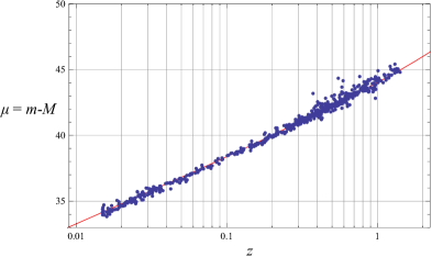
Figure 1: Dots: Observations of distance moduli $\displaystyle\mu=m-M$ and redshifts $\displaystyle z$ for Type Ia supernovae. $\displaystyle M$ is the absolute magnitude; it is the same for all Type Ia supernovae and it has the value -19.
Graph: The $\displaystyle(\mu,z)$-plot for our model of the universe fits well to observed values.

Present model

In the present paper we investigate a less arcane model: We view the universe as a sphere of the time- dependent radius $\displaystyle R(t)$ filled with matter and floating freely in infinite empty space. The matter is supposed to be distributed isotropically with respect to the center of the sphere and it is considered as a dust gas so that pressure and internal energy are negligible and temperature plays no role. Cosmic radiation is neglected as well and thus the only agent dictating the motion of the dust gas is the gravitational effect on it.

The motion is governed by the Einstein equations of gravitation, – without the cosmological constant $\displaystyle\Lambda$. We solve these equations for appropriate boundary conditions, – in the center, at infinity, and at $\displaystyle R(t)$ –, and for appropriate initial conditions at some time $\displaystyle t_{i}$ in the past, when the expansion observed by Hubble is already in progress. The initial conditions are choosen so as to provide a good fit between the calculated $\displaystyle\mu(z)$-curve and the observed data, see Fig. 1; the method is known in mathematics as the solution of an inverse problem. From the initial time onwards we follow the continued expansion for $\displaystyle t>t_{i}$ and, calculating backwards for $\displaystyle t<t_{i}$, we see that the universe has emerged from a sphere with the Schwarzschild radius.

We come to the conclusion that the observed $\displaystyle\mu(z)$-data are compatible with different solutions of the Einstein equations,– always without $\displaystyle\Lambda$. That is to say that different initial data lead to the same $\displaystyle\mu(z)$-curve. We exhibit two solutions explicitly and none of them shows an accelerated expansion nor do they require dark energy. The non-uniqeness of the solution of our inverse problem means that more astronomical observations are required to find a unique solution. Which additional observations are feasible? And which solutions of the Einstein equations describe them well? Those questions represent the cosmological conundrum.

In our paper we choose Schwarzschild coordinates $\displaystyle\left(t,r,\vartheta,\varphi\right)$ for calculations, i.e. for the formulation and reformulation and solution of the Einstein equations. In these coordinates we have a fairly simple diagonal metric tensor with only the radial and the temporal component as initially unknown functions of $\displaystyle t$ and $\displaystyle r$, while the angular components are like those in Euclidean space. For the interpretation of the results we replace the Schwarzschild coordinate time $\displaystyle t$ by the proper time of the observer in the center of the sphere.

It is true that in our model of the universe we, the observers of luminosities and redshifts, are situated in the center of the spherical dust gas or close to it. This violates the cosmological principle, according to which we should not occupy a privileged place in the cosmos. We do accept that violation because we believe that the privileged place is less counter-intuitive than is a hypothetical dark energy. Besides in Chapter 6 we conjecture that the position of our observer need not necessarily be restricted to the central point of the sphere, rather it may lie within a fairly extensive sphere.

2 Einstein equations

2.1 General form

The Einstein equations read (without cosmological constant)

$$G_{\alpha\beta}=8\pi\frac{\gamma}{c^{4}}T_{\alpha\beta},$$ (1)

where $\displaystyle G_{\alpha\beta}=R_{\alpha\beta}-\frac{1}{2}Rg_{\alpha\beta}$ is the Einstein tensor and $\displaystyle T_{\alpha\beta}$ is the energy-momentum tensor of the matter. $\displaystyle\gamma$ is the gravitational constant. $\displaystyle R_{\alpha\beta}$ is the Ricci tensor and $\displaystyle R=g^{\alpha\beta}R_{\alpha\beta}$ is the Ricci scalar. The Ricci tensor is related to the Christoffel symbols $\displaystyle\Gamma_{\delta\varepsilon}^{\gamma}$ which in turn are related to the metric tensor $\displaystyle g_{\mu\nu}$. We have

$$R_{\alpha\beta}=\frac{\partial\Gamma_{\alpha\lambda}^{\lambda}}{\partial x^{\beta}}-\frac{\partial\Gamma_{\alpha\beta}^{\lambda}}{\partial x^{\lambda}}+\Gamma_{\alpha\lambda}^{\gamma}\Gamma_{\beta\gamma}^{\lambda}-\Gamma_{\alpha\beta}^{\lambda}\Gamma_{\gamma\lambda}^{\gamma}\>\textrm{and}\>\Gamma_{\alpha\beta}^{\lambda}=\frac{1}{2}g^{\lambda\gamma}\left(\frac{\partial g_{\gamma\alpha}}{\partial x^{\beta}}+\frac{\partial g_{\gamma\beta}}{\partial x^{\alpha}}-\frac{\partial g_{\alpha\beta}}{\partial x^{\gamma}}\right).$$ (2)

2.2 Metric tensor. Speed and trajectory of light.

For the present purpose, – the consideration of a radially expanding sphere, isotropically filled with matter – we assume that the metric tensor has the form

$$g_{ij}=\left(\begin{array}[]{cccc}Z\\ &S\\ &&r^{2}\\ &&&r^{2}\sin^{2}\vartheta\end{array}\right).$$ (3)

Space-time coordinates $\displaystyle\left(t,r,\vartheta,\varphi\right)$ for which the metric tensor has this form are called Schwarzschild coordinates. Oppenheimer & Volkoff [14] and Oppenheimer & Snyder [15] have used Schwarzschild coordinates for the description of a neutron star. Here we use them for the description of the universe as a whole: A spherical dust gas in infinite empty space. A sphere of radius $\displaystyle r$ in Schwarzschild coordinates obviously has the surface area $\displaystyle 4\pi r^{2}$ just like in Euclidean space, see also Misner et al [13]. The components $\displaystyle Z$ and $\displaystyle S$ may be functions of $\displaystyle t$ and $\displaystyle r$, and we rely on the Einstein equations to find the dependence. $\displaystyle Z(t,r)$ must be negative, because without gravitation $\displaystyle Z$ must be equal to -1. $\displaystyle S$ must be equal to 1 in that case.

Since $\displaystyle Z(t,r)$ and $\displaystyle S(t,r)$ are components of the metric tensor, we feel justified to assume that they must be continuous and smooth functions, apart possibly from singular points.

It follows that the infinitesimal distance element $\displaystyle ds^{2}=g_{\alpha\beta}dx^{\alpha}dx^{\beta}$ in space-time is given in terms of the coordinate increments $\displaystyle dt$ and $\displaystyle dr$ by

$$ds^{2}=Zc^{2}dt^{2}+Sdr^{2}.$$ (4)

In a local and momentary Lorentz frame at rest with a particle of matter we denote the coordinate increments of time and radial distance by $\displaystyle d\theta$ and $\displaystyle d\varrho$ so that we have

$$ds^{2}=-c^{2}d\theta{}^{2}+d\varrho^{2}.$$ (5)

$\displaystyle d\theta$ and $\displaystyle d\varrho$ are called the increments of proper time and proper distance associated with the particle.

Hence follows a relation between $\displaystyle dt$ and $\displaystyle d\theta$ for fixed $\displaystyle\varrho$

$$d\theta=\sqrt{|Z|}\sqrt{1-\frac{V^{2}}{c^{2}}\frac{S}{|Z|}}dt,\>\textrm{where}\>V=\left(\frac{\partial r}{\partial t}\right)_{\varrho}$$ (6)

is the velocity of a material particle in the $\displaystyle(t,r)$-system. Similarly a relation between $\displaystyle dr$ and the increment $\displaystyle d\varrho$ of proper distance at fixed $\displaystyle\theta$ reads

$$d\varrho=\sqrt{S}\sqrt{1-\frac{V^{2}}{c^{2}}\frac{S}{|Z|}}dr.$$ (7)

The trajectory of a radial light ray in the $\displaystyle(t,r)$-system is governed by the equation $\displaystyle ds^{2}=0$ so that, by (4), we have for the velocity $\displaystyle c_{x}$ of light moving radially

$$\left(\frac{\partial r}{\partial t}\right)_{s}=c_{x}=\pm c\sqrt{\frac{|Z|}{S}}.$$ (8)

$\displaystyle|c_{x}|$ denotes the speed of light in the $\displaystyle(t,r)$-system. Obviously, from (6), (7) the speed $\displaystyle V$ of a material particle is bound by the speed of light in the $\displaystyle(t,r)$-system

$$|V|\leq c_{x}=c\sqrt{\frac{|Z|}{S}}.$$ (9)

Later we shall be interested in the trajectory of a light ray that reaches the observer of our spherical universe in the center of the sphere at the present time $\displaystyle t=0$, i.e. at the event $\displaystyle(t,r)=(0,0)$. That trajectory – denoted by $\displaystyle r_{T}(t)$ – must be obtained by integration from (8). Naturally we need explicit functions $\displaystyle Z(t,r)$ and $\displaystyle S(t,r)$ for the purpose. Therefore such a calculation has to be postponed until we have obtained those functions from the Einstein equations.

2.3 Specific form of the Einstein tensor

It is a cumbersome task to calculate the Christoffel symbols, hence the Ricci tensor, and hence the Einstein tensor from the specific form (3) of $\displaystyle g_{\alpha\beta}$. However, when the calculations are done, it turns out that the Einstein tensor contains only four essential non-zero components and they read

$$\begin{array}[]{ccl}G_{00}&=&\frac{1}{r^{2}}\frac{Z}{S}\left(1-S-r\frac{S^{\prime}}{S}\right)\\ G_{0r}&=&\frac{1}{r}\frac{1}{c^{2}}\frac{\dot{S}}{S}\\ G_{rr}&=&\frac{1}{r^{2}}\left(1-S+r\frac{Z^{\prime}}{Z}\right)\\ G_{\vartheta\vartheta}&=&r^{2}\frac{1}{4c^{2}}\frac{1}{ZS}\left(2\ddot{S}-\frac{1}{S}\dot{S}^{2}-\frac{1}{Z}\dot{Z}\dot{S}+2c^{2}Z^{\prime\prime}-c^{2}\frac{1}{Z}Z^{\prime 2}-\frac{1}{S}S^{\prime}Z^{\prime}-\frac{2c^{2}}{r}\left(Z^{\prime}-\frac{Z}{S}S^{\prime}\right)\right).\end{array}$$ (10)

$\displaystyle\left(\right)^{\prime}$ and $\displaystyle\left(\right)^{\bullet}$ denote partial derivatives with respect to $\displaystyle r$ and $\displaystyle t$ respectively. $\displaystyle G_{\varphi\varphi}$ is not zero, but it is equal to $\displaystyle G_{\vartheta\vartheta}$ to within a factor $\displaystyle r^{2}\sin^{2}\vartheta$ and may therefore be ignored, because the components $\displaystyle T_{\vartheta\vartheta}$ and $\displaystyle T_{\varphi\varphi}$ of the energy-momentum tensor both vanish in our case as we shall presently see.

2.4 Energy-momentum tensor for a dust gas

We assume that the matter in the sphere is a dust gas. This means that there are no viscosities and, in addition, that the pressure may be neglected. If that is true, the energy-momentum tensor is given by

$$T_{\alpha\beta}=\sigma U_{\alpha}U_{\beta},$$ (11)

where $\displaystyle\sigma$ is a scalar rest-mass density of the matter. The idea is, of course, that the matter in the universe is "smeared out" to form a continuum; each point is then occupied by a "particle" of matter in the sense of continuum mechanics.

$\displaystyle U_{\alpha}$ are the covariant components of the four-velocity and $\displaystyle U^{\alpha}=g^{\alpha\beta}U_{\beta}$ are its contravariant components. For radial expansion we have

$$U^{\alpha}=\frac{dx^{\alpha}}{d\theta}=\frac{dx^{\alpha}}{dt}\frac{dt}{d\theta}=\left(\begin{array}[]{c}c\\ V\\ 0\\ 0\end{array}\right)\frac{dt}{d\theta}.$$ (12)

$\displaystyle V=\left(\frac{\partial r}{\partial t}\right)_{\varrho}$ is the radial velocity of the gas as before, and $\displaystyle\theta$ is the proper-time. We use (6) and (8) to write (12) in the form

$$U^{\alpha}=\left(\begin{array}[]{c}c\\ V\\ 0\\ 0\end{array}\right)\frac{\frac{1}{\sqrt{|Z|}}}{\sqrt{1-\frac{V^{2}}{c_{x}^{2}}}}\>\textrm{and therefore}\>U_{\alpha}=\left(\begin{array}[]{c}-c|Z|\\ VS\\ 0\\ 0\end{array}\right)\frac{\frac{1}{\sqrt{|Z|}}}{\sqrt{1-\frac{V^{2}}{c_{x}^{2}}}}.$$ (13)

Note that the $\displaystyle r$-component $\displaystyle\left(\frac{\partial r}{\partial\theta}\right)_{\varrho}$ of the 4-velocity equals

$$\left(\frac{\partial r}{\partial\theta}\right)_{\varrho}=\frac{1}{\sqrt{|Z|}}\frac{V}{\sqrt{1-\frac{V^{2}}{c_{x}^{2}}}}$$

so that $\displaystyle|\left(\frac{\partial r}{\partial\theta}\right)_{\varrho}|$ varies between 0 and $\displaystyle\infty$ when $\displaystyle|V|$ varies between 0 and $\displaystyle|c_{x}|$, the speed of light.

By (11), (13) the energy-momentum tensor assumes the form

$$T_{\alpha\beta}=\left(\begin{array}[]{cccc}\frac{\sigma c^{2}|Z|}{1-\frac{V^{2}}{c_{x}^{2}}}&\frac{-\sigma cVS}{1-\frac{V^{2}}{c_{x}^{2}}}&0&0\\ \\ \frac{-\sigma cVS}{1-\frac{V^{2}}{c_{x}^{2}}}&\frac{\sigma V^{2}\frac{S^{2}}{|Z|}}{1-\frac{V^{2}}{c_{x}^{2}}}&0&0\\ 0&0&0&0\\ 0&0&0&0\end{array}\right).$$ (14)

2.5 Specific form of the Einstein equations

Elimination of $\displaystyle G_{\alpha\beta}$ and $\displaystyle T_{\alpha\beta}$ between (1), (10), and (14) gives the specific form of the Einstein equations for the radial expansion of an isotropic sphere filled by a dust gas. We obtain

$$\begin{array}[]{ccl}S^{\prime}&=&\frac{1}{r}S(1-S)+\frac{2}{r}\frac{\gamma}{c^{2}}m^{\prime}S^{2},\>\textrm{where}\>m^{\prime}\equiv\frac{\sigma 4\pi r^{2}}{1-\frac{V^{2}}{c_{x}^{2}}}\\ \dot{S}&=&-\frac{2}{r}\frac{\gamma}{c^{2}}m^{\prime}VS^{2}\\ Z^{\prime}&=&-\frac{1}{r}Z(1-S)-\frac{2}{r}\frac{\gamma}{c^{2}}m^{\prime}S^{2}\frac{V^{2}}{c^{2}}\\ 0&=&-2\ddot{S}+\frac{1}{S}\dot{S}^{2}+\frac{1}{Z}\dot{Z}\dot{S}-2c^{2}Z^{\prime\prime}-c^{2}\frac{1}{Z}Z^{\prime 2}+c^{2}\frac{1}{S}S^{\prime}Z^{\prime}-\frac{2c^{2}}{r}\left(Z^{\prime}-\frac{Z}{S}S^{\prime}\right).\end{array}$$ (15)

We rely on these four equations for the determination of the four fields $\displaystyle Z(t,r)$, $\displaystyle S(t,r)$, $\displaystyle\sigma(t,r)$, and $\displaystyle V(t,r)$. First, however, we rewrite these equations aiming for a set of equations that can be recognized as a relativistic generalization of the Newtonian – non relativistic – set appropriate for a self-gravitating dust gas.

First of all we note that (15)₁ may be written in the form

$$\left[r\left(\frac{1}{S}-1\right)\right]^{{}^{\prime}}=-2\frac{\gamma}{c^{2}}m^{\prime}$$

or, by integration from 0 to $\displaystyle r$ with $\displaystyle m(t,r)=\int_{0}^{r}m^{\prime}(t,\alpha)d\alpha$

$$S=\frac{1}{1-2\frac{\gamma}{c^{2}}\frac{m}{r}}.$$ (16)

$\displaystyle m$ is the mass within a sphere of radius $\displaystyle r$. Indeed, we observe that the integrability condition for $\displaystyle S$ implied by (15)_1,2 reads

$$\dot{m}^{\prime}+\left(m^{\prime}V\right)^{\prime}=0.$$ (17)

It follows that $\displaystyle m^{\prime}$ is the density of a conserved quantity. Therefore $\displaystyle m^{\prime}$ is the mass density of a spherical shell referred to the thickness $\displaystyle dr$ of the shell. [$\displaystyle m^{\prime}$ must not be confused with the scalar rest-mass density which is denoted by $\displaystyle\sigma$, cf. (15)₁.] Thus, by (16) the dependent field $\displaystyle S(t,r)$ may be replaced by the more intuitively appealing field $\displaystyle m(t,r)$. This field satisfies a very simple differential equation which we derive as follows. We observe that (15)₁ multiplied by $\displaystyle V$ and added to (15)₂ provides the relation

$$\left[\ln\frac{S}{S-1}\right]^{\centerdot}+V\left[\ln\frac{S}{S-1}\right]^{{}^{\prime}}=-\frac{V}{r},\>\textrm{or by (\ref{eq:S_from_m_r})}$$

$$\left[\ln\frac{m}{r}\right]^{\centerdot}+V\left[\ln\frac{m}{r}\right]^{{}^{\prime}}=-\frac{V}{r},\>\textrm{or, finally}$$

$$\dot{m}+Vm^{\prime}=0.$$

It follows that the mass inside a spherical surface of radius $\displaystyle r$ is constant for the observer moving with that surface. That result is eminently plausible, of course, and we write it as

$$\frac{dm}{dt}=0,\>\textrm{where}\>\frac{d\left(\right)}{dt}=\left(\right)^{\centerdot}+V\left(\right)^{\prime}.$$ (18)

The formidable equation (15)₄ may be given a somewhat more intuitively appealing form by elimination of $\displaystyle\ddot{S}$, $\displaystyle Z^{\prime\prime}$, $\displaystyle\dot{S}$, $\displaystyle S^{\prime}$ and by use of (16), (17). We obtain after some calculation

$$\frac{dV}{dt}-\frac{1}{2}\frac{V}{Z}\frac{dZ}{dt}=\gamma\frac{m}{r^{2}}\left(Z+2\frac{V^{2}}{c^{2}}\frac{1}{1-\frac{2\gamma}{c^{2}}\frac{m}{r}}\right).$$ (19)

This equation may be seen as the relativistic generalization of the equation of motion of a self-gravitating dust gas. Indeed, in the non-relativistic case, i.e. when $\displaystyle Z=-1$ and $\displaystyle V^{2}/c^{2}\approx 0$, we obtain from (19)

$$\frac{dV}{dt}=-\gamma\frac{m}{r^{2}},$$

which is the $\displaystyle r$-component of the non-relativistic equation of motion with the classical attractive gravitational acceleration on the right-hand-side. If an expansion is in progress, so that $\displaystyle V>0$ for all $\displaystyle r>0$ holds, that term decelerates the expansion. Note however, that in (19) the second term on the right-hand-side is positive, i.e. that term causes an accelerated expansion. In Section 5.5 the effect of that term is made explicit after the Einstein equations have been solved and the fields $\displaystyle Z(t,r)$, $\displaystyle m(t,r)$, $\displaystyle\sigma(t,r)$, and $\displaystyle V(t,r)$ have been determined. Note also that the second term on the right-hand-side of (19) becomes singular when the sphere has the radius $\displaystyle r_{S}=2\gamma M/c^{2}$ which is the Schwarzschild radius for the total mass $\displaystyle M$.

Finally we may eliminate the acceleration $\displaystyle dV/dt$ from (19) by use of (15)₁, the definition of $\displaystyle m^{\prime}$. Making use of (17), (18) we thus obtain

$$\frac{d\sigma}{dt}+\sigma V^{\prime}+2\sigma\frac{V}{r}=\frac{2\gamma}{c^{2}}\frac{m}{r^{2}}\frac{1}{1-\frac{2\gamma}{c^{2}}\frac{m}{r}}\sigma V$$ (20)

or

$$\left(\sigma r^{2}\right)^{\bullet}+\left(\sigma r^{2}V\right)^{{}^{\prime}}=\frac{2\gamma}{c^{2}}m\frac{1}{1-\frac{2\gamma}{c^{2}}\frac{m}{r}}\sigma V.$$ (21)

This is clearly the relativistic generalization of the non-relativistic law of mass-conservation, since the right-hand-side is negligible in that case. Note that non-relativistically there is no essential difference between $\displaystyle\sigma r^{2}$ and the mass density $\displaystyle m^{\prime}$.

In summary we may now say that so far the original four Einstein equations are replaced by the four equations

$$\begin{array}[]{lcl}\textrm{{From (\ref{eq:specific-form-Einstein-eqn}$\displaystyle)_{1}$with (\ref{eq:S_from_m_r}):}}&&\frac{V^{2}}{c^{2}}=Z\left(1-\frac{2\gamma}{c^{2}}\frac{m}{r}\right)\frac{\sigma 4\pi r^{2}-m^{\prime}}{m^{\prime}}\\ \textrm{From (\ref{eq:specific-form-Einstein-eqn}$\displaystyle)_{3}$with (\ref{eq:S_from_m_r}) and (\ref{eq:specific-form-Einstein-eqn}$\displaystyle)_{1}$:}&&\frac{Z^{\prime}}{Z}=\frac{\frac{2\gamma}{c^{2}}\frac{m}{r^{2}}}{1-\frac{2\gamma}{c^{2}}\frac{m}{r^{2}}}\left(1-\frac{\sigma 4\pi r^{2}-m^{\prime}}{\frac{m}{r}}\right)\\ \textrm{From (\ref{eq:specific-form-Einstein-eqn}$\displaystyle)_{1}$and (\ref{eq:specific-form-Einstein-eqn}$\displaystyle)_{2}$:}&&\frac{dm}{dt}=0\\ \textrm{From (\ref{eq:specific-form-Einstein-eqn}$\displaystyle)_{4}$:}&&\frac{dV}{dt}-\frac{1}{2}\frac{V}{Z}\frac{dZ}{dt}=\gamma\frac{m}{r^{2}}\left(Z+2\frac{V^{2}}{c^{2}}\frac{1}{1-\frac{2\gamma}{c^{2}}\frac{m}{r}}\right).\end{array}$$ (22)

Alternatively – replacing (22)₁ by its corollary (20) – we may write this set of equations as

$$\begin{array}[]{l}\frac{d\sigma}{dt}+\sigma V^{\prime}+2\sigma\frac{V}{r}=\frac{2\gamma}{c^{2}}\frac{m}{r^{2}}\frac{1}{1-\frac{2\gamma}{c^{2}}\frac{m}{r}}\sigma V\\ \frac{Z^{\prime}}{Z}=\frac{\frac{2\gamma}{c^{2}}\frac{m}{r^{2}}}{1-\frac{2\gamma}{c^{2}}\frac{m}{r^{2}}}\left(1-\frac{\sigma 4\pi r^{2}-m^{\prime}}{\frac{m}{r}}\right)\\ \frac{dm}{dt}=0\\ \frac{dV}{dt}-\frac{1}{2}\frac{V}{Z}\frac{dZ}{dt}=\gamma\frac{m}{r^{2}}\left(Z+2\frac{V^{2}}{c^{2}}\frac{1}{1-\frac{2\gamma}{c^{2}}\frac{m}{r}}\right).\end{array}$$ (23)

Yet another arrangement of these equations is as follows

$$\begin{array}[]{l}\frac{V^{2}}{c^{2}}=Z\left(1-\frac{2\gamma}{c^{2}}\frac{m}{r}\right)\frac{\sigma 4\pi r^{2}-m^{\prime}}{m^{\prime}}\\ \frac{Z^{\prime}}{Z}=\frac{\frac{2\gamma}{c^{2}}\frac{m}{r^{2}}}{1-\frac{2\gamma}{c^{2}}\frac{m}{r^{2}}}\left(1-\frac{\sigma 4\pi r^{2}-m^{\prime}}{\frac{m}{r}}\right)\\ \frac{dm}{dt}=0\\ \frac{d\sigma}{dt}+\sigma V^{\prime}+2\sigma\frac{V}{r}=\frac{2\gamma}{c^{2}}\frac{m}{r^{2}}\frac{1}{1-\frac{2\gamma}{c^{2}}\frac{m}{r}}\sigma V.\end{array}$$ (24)

This results from replacing (22)₄ by its corollary (20). The three sets (22) through (24) are equivalent; their different forms are needed here for arguments of interpretation and in the numerical solution of the set.

2.6 Non-dimensional variables

For the subsequent numerical calculations we introduce dimensionless dependent and independent variables based on the speed of light $\displaystyle c$, the total mass $\displaystyle M$ of the universe and its present radius $\displaystyle R(0)$. Note that both $\displaystyle M$ and $\displaystyle R(0)$ are a priori unknown; they must be chosen so as to be compatible with the $\displaystyle\mu(z)$-curve. We define

$$\hat{r}=\frac{r}{R(0)},\;\hat{t}=\frac{ct}{R(0)},\;\hat{R}=\frac{R}{R(0)},\;\hat{\sigma}=\frac{\sigma\frac{4\pi}{3}R^{3}(0)}{M},\;\hat{m}=\frac{m}{M},\;\hat{V}=\frac{V}{c},\;\hat{c}_{x}=\frac{c_{x}}{c}.$$ (25)

Also we introduce the dimensionless parameter

$$Q=\frac{2\gamma}{c^{2}}\frac{M}{R(0)},$$ (26)

which represents the Schwarzschild radius of the universe referred to its present radius $\displaystyle R(0)$.

3 External solution for S(t,r) and Z(t,r)

In the space outside the matter-filled sphere the rest mass density $\displaystyle\sigma$ is equal to zero so that (15)₁ may be integrated to give $\displaystyle S=K(t)/(1-K(t)/r)$. $\displaystyle K(t)$ is a constant of integration whose value is given by (16) as $\displaystyle\left(2\gamma/c^{2}\right)M$ , because at the surface of the sphere $\displaystyle S$ must be continuous and equal to the value given by (16) with $\displaystyle m=M\equiv m(t,R(t))$ which is the constant total mass. Thus we have for the external solution of $\displaystyle S$

$$S_{ext}=\frac{1}{1-\frac{2\gamma}{c^{2}}\frac{M}{r}}\>\textrm{for}\>r>R(t),\>\textrm{or}\>S_{ext}=\frac{1}{1-Q\frac{1}{\hat{r}}}\>\textrm{for}\>\hat{r}>\hat{R}(\hat{t}).$$ (27)

If we require $\displaystyle S(t,r)$ to be continuous and smooth at the surface, we must obviously have $\displaystyle m^{\prime}(t,R(t))=0$.

$\displaystyle Z_{ext}$, the outer solution of $\displaystyle Z(t,r)$, follows by insertion of (27) into (22)₂, and integration: $\displaystyle Z_{ext}=k(t)\left(1-\frac{2\gamma}{c^{2}}\frac{M}{r}\right)$, where $\displaystyle k(t)$ is a constant of integration whose value must be equal to $\displaystyle-1$, so that $\displaystyle Z\rightarrow-1$ for $\displaystyle r\rightarrow\infty$, where gravitation is negligible. Thus we have for the outer solution of $\displaystyle Z$

$$Z_{ext}=-1+\frac{2\gamma}{c^{2}}\frac{M}{r}\>\textrm{for}\>r>R(t)\;\textrm{or}\;Z_{ext}=-1+Q\frac{1}{\hat{r}}\>\textrm{for}\>\hat{r}>\hat{R}(\hat{t}).$$ (28)

Neither $\displaystyle S_{ext}$ nor $\displaystyle Z_{ext}$ depend on time. And obviously $\displaystyle S_{ext}$ is singular at

$$r=r_{S}\equiv\frac{2\gamma}{c^{2}}M,\;\textrm{or}\;\hat{r}=\hat{r}_{S}=Q,$$ (29)

and $\displaystyle Z$ is equal to zero at that radius which is known as the Schwarzschild radius. Therefore the metric (3) loses its meaning there.

4 Internal solutions

4.1 Distance modulus and redshift

The distance modulus $\displaystyle\mu$ and the redshift $\displaystyle z$ of Type Ia supernovae represent reliable information from which we may infer some knowledge about the structure and motion of the universe, see Fig 1. That information comes to us at the event $\displaystyle(t,r)=(0,0)$ through the light of stars which was emitted in the past at events $\displaystyle(t,r_{T}(t))$ with $\displaystyle t<0$ and with $\displaystyle 0<r_{T}(t)<R(t)$. $\displaystyle r_{T}(t)$ is the trajectory of light introduced in Section 2.2. $\displaystyle\mu$ and $\displaystyle z$ depend on the values of the fields $\displaystyle\sigma$, $\displaystyle m$, $\displaystyle Z$ and $\displaystyle V$ at the event $\displaystyle(t,r_{T}(t))$ of emission and for our model that dependence is given by the functions

$$\begin{array}[]{c}z(t)=z(t,r_{T}(t))=\sqrt{\frac{S(0,0)}{S(t,r_{T}(t))}}\sqrt{\frac{1+\frac{V(t,r_{T}(t))}{\underset{x}{c}(t,r_{T}(t))}}{1-\frac{V(t,r_{T}(t))}{\underset{x}{c}(t,r_{T}(t))}}}-1,\\ \mu(t)=\mu(t,r_{T}(t))=5\log_{10}\left[\frac{1}{10\textrm{pc}}r_{T}(t)\sqrt{\frac{S(t,r_{T}(t))}{S(0,0)}}(1+z)^{2}\right].\end{array}$$ (30)

These equations are derived in the Appendix, see (51) and (55)₂ respectively. Therefore our model of the universe – if it is valid – must have solutions $\displaystyle\sigma(t,r)$, $\displaystyle m(t,r)$ (or $\displaystyle S(t,r)$), $\displaystyle Z(t,r)$, and $\displaystyle V(t,r)$ which are consistent with the observed luminosities and redshifts. Such solutions will be found in this chapter.

4.2 Initial conditions $\displaystyle\hat{\sigma}(\hat{t}_{i},\hat{r})$ and $\displaystyle\hat{m}(\hat{t}_{i},\hat{r})$

We take the initial time as some $\displaystyle t_{i}<0$ and our plan is to calculate forward from there into the range $\displaystyle t>t_{i}$ and backwards into the range $\displaystyle t<t_{i}$. Inspection of (22)_1,2 shows that we need to impose initial conditions $\displaystyle\hat{\sigma}(\hat{t}_{i},\hat{r})$ and $\displaystyle\hat{m}(\hat{t}_{i},\hat{r})$ in order to determine $\displaystyle\hat{Z}(\hat{t}_{i},\hat{r})$ and $\displaystyle\hat{V}(\hat{t}_{i},\hat{r})$, the former by integration of (22)₂. The constant of integration may be found by the assumed continuity of $\displaystyle Z$ at the surface $\displaystyle R(t_{i})$ of the initial sphere. But smoothness of $\displaystyle Z$ – also assumed – needs restrictions on the initial functions $\displaystyle\hat{\sigma}(\hat{t}_{i},\hat{r})$ and $\displaystyle\hat{m}(\hat{t}_{i},\hat{r})$; by (22)_1,2 it requires that $\displaystyle\hat{\sigma}(\hat{t}_{i},\hat{R}(t_{i}))$ and $\displaystyle\left.\frac{\partial\hat{m}}{\partial\hat{r}}\right|_{\left(\hat{t}_{i},\hat{R}(t_{i})\right)}$ both vanish. Also, obviously, we must have $\displaystyle\hat{m}(\hat{t}_{i},0)=0$ and $\displaystyle\hat{m}(\hat{t}_{i},\hat{R}(t_{i}))=1$ and, for reasons of symmetry, $\displaystyle\left.\frac{\partial\hat{\sigma}}{\partial\hat{r}}\right|_{(\hat{t},0)}=0$ and $\displaystyle\hat{V}(\hat{t},0)=0$. Finally, by (22)₁, $\displaystyle\left.\frac{\partial\hat{m}}{\partial\hat{r}}\right|_{(\hat{t},\hat{r})}$ must be bigger than $\displaystyle 3\hat{\sigma}(\hat{t},\hat{r})4\pi\hat{r}^{2}$ for all times and all radii, lest $\displaystyle V^{2}$ be negative.

Apart from these conditions $\displaystyle\hat{\sigma}(\hat{t}_{i},\hat{r})$ and $\displaystyle\hat{m}(\hat{t}_{i},\hat{r})$ are arbitrary or, at least, there is nothing in the theory that would restrict their generality. Such a circumstance is commonplace in the solution of partial differential equations, the situation merely needs the input of observed – or otherwise given – initial data. Here, however, in an application of partial differential equations to the universe, there is a problem: Observations are either impossible or insufficient. For instance an observer at the event $\displaystyle(t_{i},0)$ cannot possibly measure $\displaystyle\sigma(t_{i},r)$, because light with its finite speed needs time to travel from $\displaystyle r$ to the center at $\displaystyle r=0$.

In this situation we have to determine the initial conditions $\displaystyle\hat{\sigma}(\hat{t}_{i},\hat{r})$ and $\displaystyle\hat{m}(\hat{t}_{i},\hat{r})$ in a complex argumentative loop as follows. We assume trial functions $\displaystyle\hat{\sigma}_{trial}(\hat{t}_{i},\hat{r})$, $\displaystyle\hat{m}_{trial}(\hat{t}_{i},\hat{r})$ and determine the corresponding solution $\displaystyle\hat{\sigma}(\hat{t},\hat{r})$, $\displaystyle\hat{m}(\hat{t},\hat{r})$, $\displaystyle\hat{Z}(\hat{t},\hat{r})$, $\displaystyle\hat{V}(\hat{t},\hat{r})$ of the Einstein equations, hence the trajectory $\displaystyle r_{T}(t)$ and hence the distance modulus $\displaystyle\mu(\hat{t},\hat{r}_{T}(\hat{t}))$ and the redshift $\displaystyle z(\hat{t},\hat{r}_{T}(\hat{t}))$ from (30) and finally $\displaystyle\mu(z)$ by elimination of $\displaystyle\hat{t}$. If the agreement with the observed $\displaystyle\mu(z)$-relation is good, so were the trial functions. If not, we have to change the trial functions and try again until we have a satisfactory agreement.

Such a procedure is known as the solution of an inverse problem, a complex variant of the simple shooting method. It is a cumbersome and time-consuming process. However, it can be automated to a certain extent. Also the process may be abbreviated by an intelligent choice of the trial functions and it may be directed by intermediate results. If well-conducted, the process in the end amounts to the adjustment of a few parameters to the observed data.

As specific trial functions for $\displaystyle\hat{\sigma}(\hat{t}_{i},\hat{r})$ and $\displaystyle\hat{m}(\hat{t}_{i},\hat{r})$ we choose

$$\begin{array}[]{l}\hat{\sigma}_{trial}(\hat{t}_{i},\hat{r})=\hat{\sigma}(\hat{t}_{i},0)\left(1-\left(\frac{\hat{r}}{\hat{R}(\hat{t}_{i})}\right)^{2n}\right)\left(1-a\left(\frac{\hat{r}}{\hat{R}(\hat{t}_{i})}\right)^{2}\right),\;\textrm{with}\;n\geq 2,\>a\leq 1\\ \left.\frac{\partial\hat{m}_{trial}}{\partial\hat{r}}\right|_{(\hat{t}_{i},\hat{r})}=3\hat{\sigma}_{trial}(\hat{t}_{i},\hat{r})\hat{r}^{2}B(\hat{r}),\;\textrm{where}\;B(\hat{r})=\frac{1}{1-\left(b_{1}\hat{r}+b_{3}\hat{r}^{3}+b_{5}\hat{r}^{5}\right)^{2}}.\end{array}$$ (31)

$\displaystyle\hat{m}_{trial}(\hat{t}_{i},\hat{r})$ itself follows by integration of (31)₂ over $\displaystyle\hat{r}$ between 0 and $\displaystyle\hat{r}$ , since $\displaystyle\hat{m}(\hat{t}_{i},0)=0$ holds. And $\displaystyle\hat{\sigma}(\hat{t}_{i},0)$ may be calculated from the requirement that $\displaystyle\hat{m}(\hat{t}_{i},\hat{R}(\hat{t}_{i}))$ be equal to 1. Fairly obviously the trial functions obey all the conditions we have required. In particular, the form of $\displaystyle B(\hat{r})$ ensures that $\displaystyle\hat{V}^{2}\geq 0$ holds. This leaves us with five parameters in (31) to be determined in the laborious adaptive process of solution of our inverse problem, namely $\displaystyle n$, $\displaystyle a$, $\displaystyle b_{1}$, $\displaystyle b_{3}$, $\displaystyle b_{5}$. Also $\displaystyle Q$, the dimensionless Schwarzschild radius, and $\displaystyle R(0)$, the present radius, enter into this problem. Two convenient choices of the outer radius $\displaystyle\hat{R}(\hat{t}_{i})$ of the sphere at two initial times $\displaystyle\hat{t}_{i}$ are $\displaystyle\hat{R}(\hat{t}_{i})=0.44$ and $\displaystyle\hat{R}(\hat{t}_{i})=0.25$. After the calculation the corresponding times $\displaystyle t_{i}$ may be read off from Fig. 4 as $\displaystyle t_{i}=-0.677$ and $\displaystyle t_{i}=-0.789$ respectively, because $\displaystyle\hat{R}(0)$ must be equal to 1.

We do not exhibit the adaptive process in detail. However, we anticipate its result in order to be able to discuss the subsequent steps: As it turns out, the triple $\displaystyle Q$, $\displaystyle n$, $\displaystyle a$ need not necessarily be involved in the adaptation in order to obtain good results, only the $\displaystyle b$´s, and $\displaystyle\hat{R}(0)$. We find that two choices of the parameters, denoted by A and B, give nearly perfect results in the sense that the calculated function $\displaystyle\mu(z)$ lies on the observed points in the fashion demonstrated in Fig. 1. These "good" choices are listed in Table 1. And the corresponding good initial functions $\displaystyle\hat{\sigma}(\hat{t}_{i},\hat{r})$ and $\displaystyle\hat{m}(\hat{t}_{i},\hat{r})$ are exhibited in Fig. 2.

Table 1: Two "good" parameter choices in the initial conditions for $\displaystyle\hat{\sigma}(\hat{t}_{i},\hat{r})$ and $\displaystyle\hat{m}(\hat{t}_{i},\hat{r})$ at time $\displaystyle\hat{t}_{i}$.

	Q	n	a	$\displaystyle b_{1}$	$\displaystyle b_{3}$	$\displaystyle b_{5}$	$\displaystyle R(0)$
A	0.11	2	1	1.77	-0.94	17.65	$\displaystyle 10.79*10^{9}$ly
B	0.015	3	0	3.9125	0	0	$\displaystyle 14.27*10^{9}$ly

Figure 2: Initial functions $\displaystyle\hat{\sigma}(\hat{t_{i}},\hat{r})$ and $\displaystyle\hat{m}(\hat{t}_{i},\hat{r})$ for the parameter choices A (solid) and B (dashed).

The fact that there are two "good" sets of trial functions emphasizes the non-uniqueness of the solution of our inverse problem. There are sure to be many more good solutions, meaning that more astronomical observations – in addition to $\displaystyle\mu$- and $\displaystyle z$-measurements – are needed to describe the universe properly.

4.3 Initial functions for $\displaystyle Z(\hat{t}_{i},\hat{r})$ and $\displaystyle\hat{V}(\hat{t}_{i},\hat{r})$

Given $\displaystyle\hat{\sigma}(\hat{t}_{i},\hat{r})$ and $\displaystyle\hat{m}(\hat{t}_{i},\hat{r})$ we may now calculate the initial functions $\displaystyle Z(\hat{t}_{i},\hat{r})$ and $\displaystyle\hat{V}(\hat{t}_{i},\hat{r})$ from the Einstein equations (22)_1,2. Integration of (22)₂ provides $\displaystyle Z(\hat{t}_{i},\hat{r})$ and subsequent insertion of this initial function into (22)₁ provides $\displaystyle\hat{V}(\hat{t}_{i},\hat{r})$. The graphs are shown in Fig. 3.

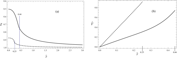
Figure 3: Initial functions for $\displaystyle Z(\hat{t}_{i},\hat{r})$ and $\displaystyle V(\hat{t}_{i},\hat{r})$ for parameter choices A (solid) and B (dashed). The graphs of $\displaystyle Z(\hat{t}_{i},\hat{r})$ combine the internal solution with the external solution (28)

4.4 Step-wise solution for $\displaystyle\hat{\sigma}(\hat{t},\hat{r})$, $\displaystyle\hat{m}(\hat{t},\hat{r})$ , $\displaystyle\hat{V}(\hat{t},\hat{r}),$ $\displaystyle\hat{Z}(\hat{t},\hat{r})$ and $\displaystyle\hat{R}(\hat{t})$

We proceed to find the solution of the Einstein equations (22), or (23), or (24). All functions depend on $\displaystyle(\hat{t},\hat{r})$.

The algebraic equation (24)₁ is only used to calculate the initial condition for $\displaystyle\hat{V}$. In order to avoid the indeterminate expression $\displaystyle(3\hat{\sigma}\hat{r}^{2}-\hat{m}^{\prime})/\hat{m}^{\prime}$ in (24)₁ at $\displaystyle\hat{r}=\hat{R}(\hat{t})$ we use the set (23) for the numerical solution instead of (24). This set represents a coupled system of three partial differential equations for $\displaystyle\hat{m}$, $\displaystyle\hat{\sigma}$, $\displaystyle\hat{V}$ and one ordinary differential equation for $\displaystyle Z$.

For a very small time step $\displaystyle\Delta\hat{t}$ we replace $\displaystyle\hat{V}$ in the equation (23)₃ by the initial condition. The result is the simple Burgers equation

$$\frac{\partial\hat{m}(\hat{t},\hat{r})}{\partial t}+\hat{V}(\hat{t}_{i},\hat{r})\frac{\partial\hat{m}(\hat{t},\hat{r})}{\partial\hat{r}}=0,$$

in which $\displaystyle\hat{m}(\hat{t},\hat{r})$ is the only unknown. For the initial condition of $\displaystyle\hat{m}$ we have $\displaystyle\hat{m}(\hat{t}_{i},\hat{r})$ by (31)₂ on the interval $\displaystyle 0\leq\hat{r}\leq\hat{R}(\hat{t}_{i})$. The solution follows by the numerical method of characteristics on the interval $\displaystyle 0\leq\hat{r}\leq\hat{R}(\hat{t}_{i}+\Delta\hat{t})$. The equation (23)₁ will also give a Burgers equation for $\displaystyle\hat{\sigma}$ by replacing $\displaystyle\hat{m}$ and $\displaystyle\hat{V}$ by their initial conditions. This equation is again solved by the numerical method of characteristics.

Now we have $\displaystyle\hat{m}(\hat{t},\hat{r})$ and $\displaystyle\hat{\sigma}(\hat{t},\hat{r})$ and these functions are inserted in the equation (23)₂ for $\displaystyle Z$, which may be solved by a standard method for ordinary differential equations.

At the end of the first time step we solve the partial differential equation (23)₄ for $\displaystyle\hat{V}$ in the same manner as the equation for $\displaystyle\hat{\sigma}$.

The solution $\displaystyle\hat{m}(\hat{t},\hat{r})$, $\displaystyle\hat{\sigma}(\hat{t},\hat{r})$, $\displaystyle Z(\hat{t},\hat{r})$, $\displaystyle\hat{V}(\hat{t}_{i},\hat{r})$ on $\displaystyle\hat{t}_{i}\leq\hat{t}\leq\hat{t}_{i}+\Delta\hat{t}$ and $\displaystyle 0\leq\hat{r}\leq\hat{R}(\hat{t}_{i}+\Delta\hat{t})$ is then used as initial condition for the next time step.

4.5 Summary of results

First and foremost the solution of the Einstein equations provides the radius of the universe as a function of time as shown in Fig. 4a. The present time $\displaystyle t=0$ is identified as the abscissa of the radius $\displaystyle\hat{R}=1$ . Thus we see that the time $\displaystyle t_{i}$, which we have arbitrarily chosen as the initial time with $\displaystyle\hat{R}(\hat{t}_{i})=0.44$ for choice A is equal to $\displaystyle\hat{t}_{i}=-0.677$, while for $\displaystyle\hat{R}(\hat{t_{i}})=0.25$ in choice B it is equal $\displaystyle\hat{t}_{i}=-0.789$. $\displaystyle\hat{R}(\hat{t})$ grows indefinitely in the future toward an asymptotic slope. Also inspection of the graph $\displaystyle\hat{R}(\hat{t})$ in the past reveals an asymptotic approach of $\displaystyle\hat{R}(\hat{t})$ toward the Schwarzschild radius $\displaystyle Q$ as $\displaystyle t$ tends to small values. Thus we conclude that the expanding universe has emerged as a sphere with that radius. Fig. 4b shows plots of $\displaystyle\hat{V}_{R}(\hat{t})$, the surface velocity of the expanding sphere which results from differentiation of $\displaystyle\hat{R}(\hat{t})$. It starts with zero velocity at small times and continues to grow asymptotically toward $\displaystyle\hat{V}_{R}=1$. The growth of $\displaystyle\hat{R}(\hat{t})$ and $\displaystyle\hat{V}_{R}(\hat{t})$ seems to be accelerating, since the slope of $\displaystyle\hat{V}_{R}(\hat{t})$ is positive and since the graph of $\displaystyle\hat{R}(\hat{t})$ is convex, i.e. it has a positive curvature; at least $\displaystyle\hat{V}_{R}(\hat{t})$ does not stop growing, as far as we can tell, even for large times. We come back to this point in Chapter 5.

Figure 4: $\displaystyle\hat{R}(\hat{t})$ and $\displaystyle\hat{V}_{R}(\hat{t})$ for parameter choices A (solid) and B (dashed)

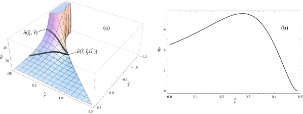
Figure 5: (a): $\displaystyle\hat{\sigma}(\hat{t},\hat{r})$. (b): $\displaystyle\hat{\sigma}(\hat{r})$ along the trajectory. Parameter choice A.

The main results of our calculation are the fields $\displaystyle\hat{\sigma}(\hat{t},\hat{r})$ , $\displaystyle\hat{m}(\hat{t},\hat{r})$ , $\displaystyle\hat{V}(\hat{t},\hat{r})$ and $\displaystyle\hat{Z}(\hat{t},\hat{r})$. Since they are fields on the $\displaystyle(t,r)$-plane, the best way to represent them is by 3-D plots. Such plots are shown in Fig. 5 through 8 for times $\displaystyle-1.5\leq\hat{t}\leq 0.5$ or $\displaystyle-2.0\leq\hat{t}\leq 0.5$ and in the interval $\displaystyle 0\leq\hat{r}\leq\hat{R}(\hat{t})$. The plots use different perspectives, depending on whatever seems most appropriate to us. All 3-D plots represent solutions for the parameter choice A.

Additional important information furnished by the Einstein equations are shown in Fig. 9, which represent the fields

$$S(t,r)\;\textrm{and}\;\left(\frac{\partial r}{\partial t}\right)_{s}=c_{x}=c\sqrt{\frac{\left|Z(t,r)\right|}{S(t,r)}},$$ (32)

$\displaystyle S(t,r)$ follows from $\displaystyle m(t,r)$ by (16) and $\displaystyle c_{x}$, the speed of light, is recalled from (8). The corresponding 3-D plots are shown in Fig. 9.

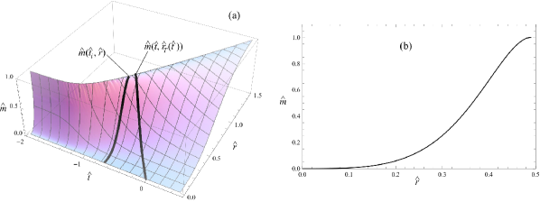
Figure 6: (a): $\displaystyle\hat{m}(\hat{t},\hat{r})$. (b): $\displaystyle\hat{m}(\hat{r})$ along the trajectory. Parameter choice A.

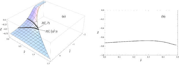
Figure 7: (a): $\displaystyle Z_{int}(\hat{t},\hat{r})$. (b): $\displaystyle Z(\hat{r})$ along the trajectory. Parameter choice A.

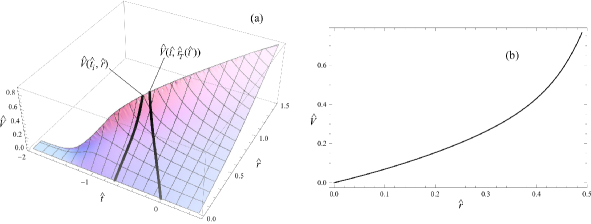
Figure 8: (a): $\displaystyle\hat{V}(\hat{t},\hat{r})$. (b): $\displaystyle\hat{V}(\hat{r})$ along the trajectory. Parameter choice A.

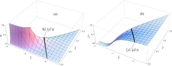
Figure 9: (a):$\displaystyle S(\hat{t},\hat{r})$. (b): $\displaystyle\hat{c}_{x}(\hat{t},\hat{r})$. Parameter choice A

Fig. 9b represents the speed of light at every event $\displaystyle(t,r)$. Starting from the event $\displaystyle(t,r)=(0,0)$ we may thus determine – by numerical integration – the past trajectory $\displaystyle r_{T}(t)$ of a light ray that reaches the center at the present time. That trajectory is shown in Fig. 10, see also Fig. 22 in the Appendix, Chapter 7. It is only from points on this trajectory that we, at $\displaystyle(0,0)$, can receive information about light-emitting stars.

The 3-D plots 5 through 9 exhibit the values of the fields $\displaystyle Z(t,r_{T}(t))$ through $\displaystyle\hat{c}_{x}(t,r_{T}(t))$ along the solid lines starting at $\displaystyle(t,r)=(0,0)$and ending on the surface of the sphere.

The initial values that start from $\displaystyle(\hat{t},\hat{r})=(-0.677,0)$ are also shown as solid lines in the 3-D plots 5 through 8. Note that those lines in the $\displaystyle(\hat{\sigma},\hat{t},\hat{r})$-plot and in the $\displaystyle(\hat{m},\hat{t},\hat{r})$-plot represent our trial functions (31) for the “good” parameter choice A.

The radius $\displaystyle R(t)$ and the trajectory $\displaystyle r_{T}(t)$ intersect for choice A at the event $\displaystyle(\hat{t}_{0},\hat{r}_{0})=(-0.612,0.489)$. That event is the farthest in time and space which we can observe. It occurred at a time when the size of the universe was roughly half its present size; indeed we have $\displaystyle r_{0}\approx 0.5R(0)$.

Naturally the values of our fields along the trajectory are most important for the astronomer. We denote them by $\displaystyle\hat{\sigma}(\hat{t})\equiv\hat{\sigma}(\hat{t},\hat{r}_{T}(\hat{t}))$ etc., if represented as functions of $\displaystyle\hat{t}$ with $\displaystyle\hat{t}_{0}\leq\hat{t}\leq 0$ , or as $\displaystyle\hat{\sigma}(\hat{r})$ etc., if represented as functions $\displaystyle r$ with $\displaystyle 0\leq r\leq r_{0}$.

Fig. 5b shows $\displaystyle\hat{\sigma}(\hat{r})$; it exhibits a non-monotone character due to the competing facts that $\displaystyle\sigma$ was larger in the past in an expanding universe but has to drop to zero at the surface of the universe. The starting value $\displaystyle\hat{\sigma}\approx 4$ means that the central density $\displaystyle\sigma(0,r_{T}(0))$ at the present time is four times bigger than the mean density at that time, see (25)₄.

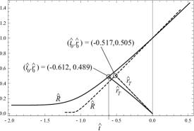
Figure 10: $\displaystyle\hat{r}_{T}(t)$ is the light trajectory. Parameter choice A (solid) and B (dashed). Note that $\displaystyle\hat{r}_{T}(t)$ is slightly concave, see also Fig. 22 in the Appendix, Chapter 7.

Note that the slope of the light trajectory in Fig. 10 is the speed of light $\displaystyle c_{x}$ at the event $\displaystyle(t,r_{T}(t))$. It is everywhere slightly smaller than $\displaystyle c$, but it grows as the central event $\displaystyle(0,0)$ is approached.

Although the 3-D plots of Figs. 5 through 9 represent the solution of the Einstein equations, it is best to postpone a discussion of its qualitative and quantitative features. Indeed, the solution is represented here in terms of Schwarzschild coordinates $\displaystyle(t,r)$. These coordinates have allowed us a fairly easy solution, but they are bad for interpretation in terms of intuitive notions of space and time, particularly time. A case in point is the asymptotic behavior of $\displaystyle R(t)$ at small times, where $\displaystyle R$ approaches the Schwarzschild radius asymptotically, whereas we expect an increasingly rapid decrease of $\displaystyle R$ toward $\displaystyle Q$ under the action of the gravitation. According to our solution, however, the derivative $\displaystyle dt/dR$ is singular for $\displaystyle R\rightarrow Q$ and that forces us to deliberate about the rates of clocks in a gravitational field as compared to their rates in a Lorentz frame. We postpone this topic because at the present stage we do not yet need it; see however Chapter 5.

What we do discuss next is the question whether our solution, – albeit in Schwarzschild coordinates –, does allow us to derive the observed $\displaystyle\mu(z)$-relation of Fig. 1 as we have anticipated. Since that relation does not explicitly contain $\displaystyle r$ and $\displaystyle t$, it is valid irrespective of our choice of space-time coordinates.

4.6 Cosmological conundrum

In the Appendix, Chapter 7, we have derived expressions for $\displaystyle z(t)$ and $\displaystyle\mu(t)$, see also (30). And now we have exhibited all functions on the right-hand-sides of these, – namely $\displaystyle r_{T}(t)$, $\displaystyle V(t,r_{T}(t))$, $\displaystyle c_{x}(t,r_{T}(t))$, $\displaystyle S(t,r_{T}(t))$ –, so that we may plot $\displaystyle z(t)$ and $\displaystyle\mu(t)$, or $\displaystyle z(r)$ and $\displaystyle\mu(r)$. Those plots are shown in Fig. 11 for choice A of the parameters. Elimination of $\displaystyle t$ or $\displaystyle r$ provides the graph $\displaystyle\mu(z)$ of Fig. 1 which fits the observed data well. This, of course, is a foregone conclusion since choice A represents a “good” choice in the sense of Table 1. And the criterion for “goodness” was a good fit of calculated values of the $\displaystyle\mu(z)$-curve with the measured data.

Figure 11: (a): $\displaystyle z(r)$. (b): and $\displaystyle\mu(r)$. Along the trajectory. Parameter choice A.

Choice B is another good choice and accordingly the $\displaystyle\mu(z)$ plot for choice B, shown in Fig. 12, is again good. In fact, to the naked eye there is no difference between Figs. 1 and 12.

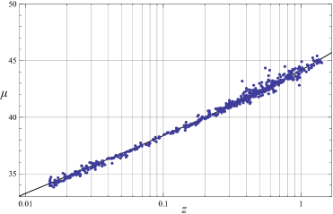
Figure 12: The $\displaystyle\mu(z)$ -plot for the parameter choice B of the universe.

We conclude that the $\displaystyle\mu(z)$ results of Figs. 1 and 12 do not call for a dark-energy-hypothesis nor do they require an accelerated expansion as we shall see in Chapter 5. That is satisfactory! But there is also non-uniqueness: Although the parameter choices A and B predict the same Hubble diagram, they do also predict different density functions $\displaystyle\sigma(t)$ or $\displaystyle\sigma(r)$ along the trajectories as is illustrated in Fig. 13. Other functions, like $\displaystyle m(r)$ or $\displaystyle Z(r)$ will differ as well between the choices A and B. This means that we need more observations; observations other than those of $\displaystyle\mu$ and $\displaystyle z$.

Figure 13: Density distribution along the trajectory. Choice A (solid), choice B (dashed).

For instance, suppose that astronomers had measured $\displaystyle\sigma(r)$ along the trajectory. We should then have to perform our inverse adjustment of initial conditions not only for the observed Hubble function $\displaystyle\mu(z)$ as the target function but also for the observed values $\displaystyle\sigma(r)$. However, $\displaystyle\sigma(r)$-observations do not seem to be available. What comes closest to them are galaxy counts.

Indeed, among the cosmological observations other than the $\displaystyle\mu(z)$-plot of Fig. 1 galaxy redshift surveys [16] have furnished a reliable histogram of the fraction of $\displaystyle 250.000$ galaxies over the redshift of the light emitted by them. The histogram has gelled into a simple smooth analytic approximation curve of the form (see [16] p. 1059ff)

$$fraction=z^{2}\exp(-49.3z^{1.55}).$$ (33)

This formula may be converted into a "smeared out" galaxy density, and there is the temptation to consider this galaxy density as proportional to the matter density $\displaystyle\sigma$. However, we are not certain whether far-away galaxies have the same mass as close ones. Therefore we have not incorporated galaxy counts – reliable as they may be – into our adaptive inverse scheme. That remains to be done in the future after more deliberation.

Moreover, it can hardly be expected that an eventual observation of $\displaystyle\sigma(r)$ would suffice to identify unique initial conditions. More observational evidence is likely to be needed and the question is: Which additional observations are feasible and what solutions do they entail? That question represents the cosmological conundrum.

5 Interpretation of results

5.1 Radius of the universe as a function of the proper time $\displaystyle\boldsymbol{\tau}\textbf{=}\boldsymbol{\theta}\textbf{(}\textbf{{t}}\textbf{,0)}$ at the center r=0.

As was mentioned before, – toward the end of Section 4.5 –, the use of Schwarzschild coordinates for the solution of the Einstein equations has made it difficult, or impossible, to interpret the results in terms of our intuitive notion of time. We believe that it is the proper time

$$\tau=\theta(t,0)$$

of the observer at the center of the universe that comes closest to our intuitive notion of time and that

$$V_{\tau}(t,r)=\left(\frac{\partial r}{\partial\tau}\right)_{\varrho}=\frac{V(t,r)}{\frac{d\tau}{dt}\left(t\right)}$$ (34)

corresponds to our intuitive notion of velocity. Therefore we proceed to replace $\displaystyle t$ by $\displaystyle\tau(t)$.

From (6) and the knowledge of $\displaystyle V(t,r)$, $\displaystyle Z(t,r)$, and $\displaystyle S(t,r)$, see Figs. 8,7,9, we obtain $\displaystyle\frac{d\theta}{dt}(t,r)$ and, in particular, the graph $\displaystyle\frac{d\tau}{dt}(t)=\frac{d\theta}{dt}(t,0)$ of Fig. 14. Integration over $\displaystyle t$ gives $\displaystyle\tau(t)$ to within a constant which we identify by requiring that $\displaystyle\tau=0$ holds for $\displaystyle t=0$. The resulting graph $\displaystyle\tau(t)$ is also shown in Fig. 14. Inspection shows that for large values of $\displaystyle t$ the proper time $\displaystyle\tau$ becomes asymptotically equal to $\displaystyle t$, while for small values of $\displaystyle t$ the proper time becomes independent of $\displaystyle t$.

Figure 14: The proper time as a function of $\displaystyle t$. Parameter choice A (solid) and B(dashed)

We conclude that sufficiently far in the past the tiniest increase of $\displaystyle\tau$ requires a large increase in $\displaystyle t$, or else: the rate of Schwarzschild coordinate clocks, which measure $\displaystyle t$, is much larger than the rate of a clock at rest in a Lorentz frame at the center. It is for this reason that the radius $\displaystyle R(t)$ in Figs. 10 and 15 does not seem to change at all with time $\displaystyle t$ as the radius approaches the Schwarzschild radius $\displaystyle Q$.

$\displaystyle R(\tau)$ on the other hand – obtained by elimination of $\displaystyle t$ between $\displaystyle R(t)$ and $\displaystyle\tau=\theta(t,0)$ – seems to grow linearly starting with $\displaystyle R=Q$, see Fig. 15a which shows both functions $\displaystyle R(t)$ and $\displaystyle R(\tau)$. Closer inspection, however, reveals that $\displaystyle R(\tau)$ is a slightly concave function so that the observer at $\displaystyle r=0$ sees a decelerating expansion in terms of his time $\displaystyle\tau$. Fig. 15b demonstrates this fact by focussing the attention on the neighborhood of the point where $\displaystyle R(\tau)$ emerges from the Schwarzschild radius; that happens at approximately $\displaystyle\tau=-0.85$. The fact is further illustrated in Fig. 16 where the velocity of expansion $\displaystyle dR(\tau)/d\tau$ is plotted. The figure shows that the velocity is a convex function and has not even developed into a straight line at $\displaystyle\tau=0$, i.e. at the present time. For large values of $\displaystyle\tau$ the surface velocity tends to a constant value $\displaystyle<1$. For choice B this is obvious from inspection of Fig. 16; for choice A we need to pursue the graph far to right in order to see it drop below the value 1.

Figure 15: Parameter choice A. Radii $\displaystyle R(t)$ and $\displaystyle R(\tau)$. Also trajectories $\displaystyle r_{T}(t)$ and $\displaystyle r_{T}(\tau)$.

Figure 16: Surface velocity $\displaystyle dR(\tau)/d\tau$ in the range $\displaystyle-0.6<\tau<0.4$ and $\displaystyle 8<\tau<11$. Choice A (solid), choice B (dashed).

The plots of Fig. 17 correspond to those of Fig. 15 except that they are calculated for the parameter choice B. For both choices, A and B, we see the same qualitative behaviour of the $\displaystyle R(\tau)$-curve. The concavity in that curve – as exhibited in Fig. 17b – is a little more pronounced for choice B than for choice A. From both figures we conclude that the expansion of the universe is decelerating, since $\displaystyle\hat{R}(\hat{\tau})$ is concave.

Figure 17: Parameter choice B. Radii $\displaystyle R(t)$ and $\displaystyle R(\tau)$. Also trajectories $\displaystyle r_{T}(t)$ and $\displaystyle r_{T}(\tau)$.

The significant difference between $\displaystyle R(t)$ and $\displaystyle R(\tau)$ in Figs. 15 and 17 – one convex and the other concave – is reminiscent of the case of a mass which drops into a black hole. That case is routinely treated in books on general relativity, e.g. see Shapiro and Teukolsky [17]. There too the distance $\displaystyle h(t)$ of the mass from the black hole tends to a finite value as the Schwarzschild radius of the mass is approached, while $\displaystyle h(\tau)$, where $\displaystyle\tau$ is the proper time of the mass, drops precipitously toward zero.

Our solution does not provide graphs for $\displaystyle R(\tau)<Q$ simply because we do not get values for $\displaystyle R(t)<Q$. What we do obtain is the proper time when the expanding sphere emerges from the Schwarzschild radius. That time may be read off from the figures as the abscissae of the end points of the $\displaystyle R(\tau)$-curve and maybe that time is appropriately called the "time of emergence." We know nothing about the period of time before that age, which was where the "big bang" happened – if it happened – and where the expansion began. Our cosmological model is not able to provide information about such phenomena, at least not in the present form.

5.2 Trajectories

The Figs. 15 and 17 also show graphs of the trajectories $\displaystyle r_{T}(t)$ and of $\displaystyle r_{T}(\tau)$; the latter results by elimination of $\displaystyle t$ between $\displaystyle r_{T}(t)$ and $\displaystyle\tau(t)$. It is only from events on these curves that we may receive information by light about the past. In analogy to Fig. 10 we denote the coordinates of the points of intersection of the graphs $\displaystyle r_{T}(\tau)$ and $\displaystyle R(\tau)$ by $\displaystyle(\tau_{0},r_{0})$. We cannot observe what happened before $\displaystyle\tau_{0}$ and at a greater distance than $\displaystyle r_{0}$. Therefore $\displaystyle\tau_{0}$ may be called a "look back time." Its value is given in Table 2 along with other interesting properties of our models.

While the trajectory $\displaystyle r_{T}(t)$ is very slightly concave, the graph $\displaystyle r_{T}(\tau)$ is straight and its slope is equal to 1 which, in dimensional terms, means that – of course – the light moving along $\displaystyle r_{T}(\tau)$ has the speed $\displaystyle c$ of light in the Lorentz frame at the center.

5.3 Some results in tabular form

We summarize some of our results in Table 2. We recall that $\displaystyle R(0)$ was also listed in Table 1 and that it was determined by adjusting our parameters to give a good agreement between theory and observation of the $\displaystyle\mu(z)$-curve. Given $\displaystyle R(0)$ the total mass follows from the definition (26) of the Schwarzschild radius.

Table 2: Some results for the parameter choice A and B

	$\displaystyle R(0)$	$\displaystyle M$	Time of emergence	$\displaystyle\tau_{0}$	$\displaystyle r_{0}$	$\displaystyle H_{0}$
A	10.79 Gly	$\displaystyle 1.514\cdot 10^{52}$kg	$\displaystyle\approx-0.85\cong-9.22$Gy	$\displaystyle\cong-5.311$Gy	$\displaystyle\cong 5.281$Gly	$\displaystyle 0.22\cdot 10^{-17}$s-1
B	14.27 Gly	$\displaystyle 0.273\cdot 10^{52}$kg	$\displaystyle\approx-1.00\cong-14.26$Gy	$\displaystyle\cong-7.212$Gy	$\displaystyle\cong 7.210$Gly	$\displaystyle 0.22\cdot 10^{-17}$s-1

The data given in the table for choices A and B differ widely. And, what is more, they differ considerably from the values provided by the currently popular FRW cosmology, where, for instance, the age of the universe is confidently given as $\displaystyle-13.7$Gy. Well, we can only say that that value is heavily dependent on the Robertson-Walker model along with the concept of a hypothetical dark energy which, moreover, makes up 70% (!) of all mass in the universe. We do not consider that notion convincing.

5.4 Hubble´s law

The very fact that the function $\displaystyle t=t(\tau)$, according to Fig. 14, has a singularity for $\displaystyle\tau\approx-0.85$ disqualifies $\displaystyle t$ as an appropriate measure for time. That fact makes it impossible to interpret $\displaystyle V(t,r)=\left(\frac{\partial r}{\partial t}\right)_{\varrho}(t,r)$ as a reasonable measurable velocity. Therefore we ought to reformulate the calculated field $\displaystyle V(t,r)$ in terms of the proper time of the observer in the center. As in (34), we consider

$$V_{\tau}(t,r)=\frac{V(t,r)}{\frac{d\tau}{dt}(t)}$$

as the proper measure of velocity. This is a function on the $\displaystyle(t,r$)-plane. From it the velocity $\displaystyle V_{\tau}(t,r_{T}(t))$ along the trajectory, i.e. the velocity of a star which has sent out light at a time $\displaystyle t<0$, may be calculated. Hence follows the velocity $\displaystyle V_{\tau}(r)$ of the star at the distance $\displaystyle r$ along the trajectory by elimination of $\displaystyle t$ between $\displaystyle V_{\tau}(t,r_{T}(t))$ and $\displaystyle r_{T}(t)$ . It is shown in Fig. 18 and we see that it increases with an increasing gradient as $\displaystyle r$ approaches the surface of the sphere so that on the surface – where $\displaystyle r=r_{0}$ – the velocity $\displaystyle V_{\tau}(r)$ is close to 1. This means that the surface moves away from us roughly with the speed of light.

Figure 18: Velocity as function of distance along the trajectory. Choice A (solid), B (dashed). The slope of the tangent may be identified with the Hubble constant.

Close to the center, where Hubble [7] made his observations, the convex curve $\displaystyle V_{\tau}(r)$ may be approximated by its tangent whose slope is the Hubble constant $\displaystyle\hat{H}_{0}=0.759$ for choice A, see Fig 18. In dimensional form this value is thus given by $\displaystyle H_{0}=\hat{H}_{0}\frac{c}{R(0)}=0.22\cdot 10^{-17}\textrm{s}^{-1}$; it is listed in Table 2. This value agrees well with the value $\displaystyle H_{0}=0.226\cdot 10^{-17}\textrm{s}^{-1}$ which is most often given in the astronomical literature, e.g. see [1].

For choice B the initial slope of the $\displaystyle V_{\tau}(r)$ curve is given by $\displaystyle\hat{H}_{0}=0.986$ which again implies $\displaystyle H_{0}=0.22\cdot 10^{-17}\textrm{s}^{-1}$ in dimensional form, see Table 2. We must not be surprised that the choices A and B agree as to the value of the Hubble constant despite their disagreement about all other values in Table 2. Because indeed, the models do agree on the $\displaystyle\mu(z$)-relation, see Figs. 1 and 12 and Hubble´s law is a corollary of that relation. We proceed to describe this point briefly.

Generally we have, by (55)₁ in the Appendix, Chapter 7

$$d_{L}=10\,\textrm{pc}\,10^{\frac{\mu(z)}{5}},$$

where $\displaystyle d_{L}$ is the luminosity distance defined in (54). For small values of $\displaystyle z$ we have from the observed data, see Figs. 1 and 12

$$\mu(z)\approx 33.38+5\log_{10}\frac{z}{0.01}.$$

Also, by (54)₁ and (51) we have for small $\displaystyle z$

$$d_{L}\approx r\;\textrm{and}\;z\approx\hat{V}_{\tau}.$$

Hence follows for the non-dimensional Hubble constant

$$\hat{H}_{0}=\frac{\hat{V}_{\tau}}{\hat{r}}=\frac{R(0)}{10\,\textrm{pc}}\frac{1}{10^{\frac{43.38}{5}}}.$$

For the dimensional Hubble constant $\displaystyle H{}_{0}=\frac{c}{R(0)}\hat{H}_{0}$ the choice-dependent factor $\displaystyle R(0)$ cancels and thus $\displaystyle H_{0}$ is the same for choices A and B: Hubble’s observations for small $\displaystyle z$ have no independent status vis-a-vis the $\displaystyle\mu(z)$ observations.

5.5 Accelerating and decelerating contributions to the expansion of the universe

We have argued that the Schwarzschild coordinate time $\displaystyle t$ is not a good measure of time and that the proper time $\displaystyle\tau=\theta(t,0)$ in the center of the sphere is better. The difference is not trivial; indeed $\displaystyle R(t)$ exhibits an accelerated growth while $\displaystyle R(\tau)$ exhibits a decelerated growth, see Section 5.1. To be sure, according to Figs. 15 and 17 both modes of growth eventually settle into a uniform expansion with a constant velocity close to that of light, see Fig. 16. This is strange in itself, quite apart from the question whether the radius in the past has been accelerated or decelerated toward that uniform value. Indeed, do we not expect – as more or less classical physicists – that there should be a continued deceleration under the effect of the gravitational attraction? In answer to this question let us discuss the role of gravity in our model; that role has so far been disguised by the unfamiliar form of the equations and by the fog raised through the numerical solution of our inverse problem.

We call the attention to (22)₄ which, after a little rearrangement and the insertion of dimensionless quantities reads

$$\frac{d\hat{V}}{d\hat{t}}=-\frac{1}{2}Q\frac{\hat{m}}{\hat{r}^{2}}+Q\frac{\hat{m}}{\hat{r}^{2}}\hat{V}^{2}\frac{1}{1-Q\frac{\hat{m}}{\hat{r}}}-\frac{1}{2}Q\frac{\hat{m}}{\hat{r}^{2}}(Z-1)+\frac{1}{2}\frac{\hat{V}}{Z}\frac{dZ}{d\hat{t}}$$ (35)

in terms of the Schwarzschild time and

$$\frac{d\tilde{V}_{\tau}}{d\tau}=-\frac{1}{2}Q\frac{\tilde{m}}{r^{2}}+Q\frac{\tilde{m}}{r^{2}}\tilde{V}_{\tau}^{2}\frac{1}{1-Q\frac{\tilde{m}}{r}}-\frac{1}{2}Q\frac{\tilde{m}}{r^{2}}\left(\frac{\tilde{Z}(\tau,r)}{\tilde{Z}(\tau,0)}-1\right)+\frac{1}{2}\tilde{V}_{\tau}\left(\frac{1}{\tilde{Z}(\tau,r)}\frac{d\tilde{Z}(\tau,r)}{d\tau}-\frac{1}{\tilde{Z}(\tau,0)}\frac{d\tilde{Z}(\tau,0)}{d\tau}\right)$$ (36)

in terms of the proper time $\displaystyle\tau(t)$.

It is clear that those equations must be identities when we insert the solution exhibited in Chapter 4, because the solution has been derived from them. However, (35) and (36) may be viewed as expressions for the accelerations $\displaystyle dV/dt$ or $\displaystyle d\tilde{V}_{\tau}/d\tau$. We concentrate on $\displaystyle d\tilde{V}_{\tau}/d\tau$, because that is the acceleration as seen by the observer in the center. The first term on the right-hand-side is the classical gravitational acceleration. It is clearly attractive because of the minus sign. But it is not alone!

Figure 19: (a) Newtonian deceleration. (b) Repulsive acceleration. (c) Terms with $\displaystyle Z$. (d) Overall deceleration along the trajectory.

Fig. 19 shows plots of the four contributions on the right hand side of (36) along the trajectory $\displaystyle r_{T}(t)$: In (a) we see the attractive classical (Newtonian) contribution, while (b) shows the repulsive second term which grows with growing velocity as the surface is approached. In (c) we have plotted the third and fourth terms, – the terms with $\displaystyle Z$ and its derivatives; those are negative and therefore attractive. Finally the fat graph (d) exhibits the entire right-hand-side of (36). We see that the classical attraction is diminished by the other terms throughout the whole spread of the universe but that it remains attractive, albeit weakly near the surface. We conclude that there is no accelerated expansion anywhere. Therefore there is no need to introduce a hypothetical dark energy to create the accelerated expansion.

Also we now understand why it is that the surface of the universe moves with a nearly constant speed for large times despite of what we are accustomed to consider as the gravitational pull. Indeed, the gravitational pull is quite small on the surface.

The parameters for which the graphs of Fig. 19 are drawn, are those of parameter choice A. For choice B we obtain smaller values – obviously reflecting the smaller mass $\displaystyle M$ of choice B – and the final value at $\displaystyle\hat{\tau}=-0.5$ remains negative: Apparently the deceleration has not come to an end yet at the surface of the sphere.

The various accelerations of Fig. 19 are all calculated for the present trajectory, i.e. the trajectory that passes through the event $\displaystyle(0,0)$. Surely the plots will look different for trajectories at earlier times. And it is even conceivable that for such earlier times the graph (d) may exhibit an overall acceleration instead of an overall deceleration. In that respect it seems worthy of note that for real early trajectories $\displaystyle Z=0$ holds and that the accelerating term (b) in Fig. 19 becomes singular, see Fig. 7a and eqn. (36). That aspect, which touches on the notion of an inflationary past period of the universe, will be the subject of a subsequent study, if the present one fares well.

In the present study the main conclusion is that there is no overall acceleration along the present trajectory and therefore there is no need for a hypothetical dark energy.

6 Remark on the cosmological principle

We are fully aware of the fact that our model of a sherical universe floating in infinite empty space violates the cosmological principle according to which we, the observers should not occupy a privileged place in the cosmos. In our model clearly the center of the sphere is privileged and yet that site is assumed to be the place of the observer.

In early cosmology the problem became urgent with Hubble’s observation that the galaxies in our neighbourhood move away from us with a speed proportional to their distance. The question was: Why are we thus privileged? That question lost some of its urgency when it was recognized that in an infinitely extended homogeneously dense matter distribution with an expansive velocity proportional to the distance from one point the matter is in fact moving away from all points in the same manner. So, in such a universe Hubble’s observation does not put us in a privileged spot.

Of course, if the universe is spherical with a finite radius and not homogeneously filled with matter – as in our case – the argument does not hold, or at least it does not hold exactly and everywhere. We may conjecture, however, that the argument does hold approximately in an inner sphere around the center where the density is nearly constant and where the matter moves away from the center in the Hubble way. Fig. 20 and 21 show that there is such an inner sphere, well pronounced for choice B and somewhat less well pronounced for choice A.

Figure 20: $\displaystyle\sigma(t,r)$ for $\displaystyle 0\leq r\leq R(t)$ at various times. (a): Choice A. (b): Choice B.

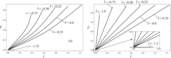
Figure 21: $\displaystyle V(t,r)$ for $\displaystyle 0\leq r\leq R(t)$ at various times. (a): Choice A. (b): Choice B.

Clearly that argument needs strengthening. It is offered here loosely so as to anticipate the objection that our model of the universe places the observer in the central point of the universe. We believe that the model is still good, if the observer is placed anywhere within the inner sphere of near-homogeneous density.

7 Appendix: Redshift of Type Ia supernovae and luminosities.

7.1 Scope

The study of redshifts requires an investigation of the Doppler shift and aberration and of the gravitational frequency shift. We discuss these phenomena in the subsequent Sections 7.2 through 7.4 with (51) and Fig. 11a as the result. Section 7.5 is given to a discussion of the apparent luminosity with (55)₂ and Fig. 11b as the result. Both results (51) and (55)₂ have been anticipated in Sections 4.1 and 4.6.

The formulae for redshifts and luminosities differ between different cosmological models, because the concepts of frequency and wave length are non-trivial in relativity. Etherington [19] has studied the problem as early as 1933. See also Ellis [20] who reviews Etherington´s work as a "Golden Oldie." Still, however, there are conflicting formulae used as relations between absolute and apparent luminosities in the modern literature. Thus the relevant results of the Friedmann-Robertson-Walker model are useless for our more mundane model; there is not even a clear-cut Doppler effect in the FRW-model, see [1]. Therefore we have rederived the relevant formula in this chapter and we hope and trust that we got things right.

7.2 Dopplershift and aberration

In this chapter we consider light emitted by a star or galaxy moving with the radial velocity $\displaystyle V$ with respect to the center of the sphere and absorbed in the center.

We look at the light from three different frames of reference: i.) the local and momentary Lorentz frames $\displaystyle{z^{\alpha}}$ and $\displaystyle{z_{0}^{\alpha}}$ – with coordinates $\displaystyle{\theta\,,z^{1},z^{2},z^{3}}$ and $\displaystyle{\theta_{0}\,,z_{0}^{1},z_{0}^{2},z_{0}^{3}}$ respectively – which accompany the star and the observer and ii.) the frame $\displaystyle{x^{\alpha}}$ – with coordinates $\displaystyle{t\,,x{}^{1},x{}^{2},x{}^{3}}$ – in which we have solved the Einstein equations. It is now appropriate to introduce rectangular Cartesian spatial coordinates $\displaystyle{z^{\alpha}}$ and $\displaystyle{x^{\alpha}}$, since the light does not necessarily move in the radial direction. However, we let $\displaystyle z^{1}$ and $\displaystyle x^{1}$ point into the radial direction so that the unit vectors of propagation of the light may be given in terms of the direction angles $\displaystyle\alpha$ and $\displaystyle\beta$ by

$$\underset{z}{n}^{a}=\left(\cos\underset{z}{\alpha},\sin\underset{z}{\alpha}\cos\underset{z}{\beta},\sin\underset{z}{\alpha}\sin\underset{z}{\beta}\right)\>\textrm{and}\>\underset{x}{n}^{a}=\left(\cos\underset{x}{\alpha},\sin\underset{x}{\alpha}\cos\underset{x}{\beta},\sin\underset{x}{\alpha}\sin\underset{z}{\beta}\right).$$ (37)

Let the light locally be described as a plane wave with frequency $\displaystyle\nu$ and wave length $\displaystyle\lambda$. The space-time wave vector $\displaystyle k_{\alpha}$ is then given by

$$\underset{z}{k_{\alpha}}=2\pi\left(\frac{\underset{z}{\nu}}{c},-\frac{1}{\underset{z}{\lambda}}\underset{z}{n}^{a}\right),\>\textrm{where}\>\underset{z}{\nu}\underset{z}{\lambda}=c$$

$$\underset{x}{k_{\alpha}}=2\pi\left(\frac{\underset{x}{\nu}}{c},-\frac{1}{\underset{x}{\lambda}}\underset{x}{n}^{a}\right),\>\textrm{where}\>\underset{x}{\nu}\underset{x}{\lambda}=\underset{x}{c}.$$ (38)

We consider $\displaystyle\underset{z}{k_{\alpha}}$ as given and calculate $\displaystyle\underset{x}{k_{\alpha}}$ using the transformation matrix between the frames $\displaystyle\left\{z^{\alpha}\right\}$ and $\displaystyle\left\{x{}^{\alpha}\right\}$

$$\underset{x}{k_{\alpha}}=\frac{\partial z^{\beta}}{\partial x^{\alpha}}\underset{z}{k_{\beta}}.$$ (39)

The transformation matrix may be calculated from the invariance of the infinitesimal distance element in space-time, see (4), (5)

$$ds^{2}=-c^{2}d\theta^{2}+dz^{12}+dz^{22}+dz^{32}=Zc^{2}dt^{2}+Sdx^{12}+Sdx^{22}+Sdx^{32}.$$ (40)

The calculation provides

$$\frac{\partial z^{\beta}}{\partial x^{\alpha}}=\left(\begin{array}[]{cccc}\frac{\sqrt{\left|Z\right|}}{\sqrt{1-\frac{V^{2}}{\underset{x}{c}^{2}}}}&-\frac{V}{\underset{x}{c}}\frac{\sqrt{\left|Z\right|}}{\sqrt{1-\frac{V^{2}}{\underset{x}{c}^{2}}}}&0&0\\ -\frac{V}{\underset{x}{c}}\frac{\sqrt{S}}{\sqrt{1-\frac{V^{2}}{\underset{x}{c}^{2}}}}&\frac{\sqrt{S}}{\sqrt{1-\frac{V^{2}}{\underset{x}{c}^{2}}}}&0&0\\ 0&0&\sqrt{S}&0\\ 0&0&0&\sqrt{S}\end{array}\right).$$ (41)

As before, $\displaystyle V=\left(\frac{\partial r}{\partial t}\right)_{\varrho}$ is the velocity of the star which emits the light; it is non-negative for the expanding sphere. Insertion of (41) into (39) gives

$$\frac{\underset{x}{\nu}}{\underset{z}{\nu}}=\sqrt{\left|Z\right|}\frac{1+\frac{V}{\underset{x}{c}}\underset{z}{n}^{1}}{\sqrt{1-\frac{V^{2}}{\underset{x}{c}^{2}}}},\;\frac{\underset{x}{\nu}}{\underset{z}{\nu}}\underset{x}{n}^{1}=\sqrt{\left|Z\right|}\frac{\underset{z}{n}^{1}+\frac{V}{\underset{x}{c}}}{\sqrt{1-\frac{V^{2}}{\underset{x}{c}^{2}}}},\;\frac{\underset{x}{\nu}}{\underset{z}{\nu}}\underset{x}{n}^{2}=\sqrt{\left|Z\right|}\underset{z}{n}^{2},\;\frac{\underset{x}{\nu}}{\underset{z}{\nu}}\underset{x}{n}^{3}=\sqrt{\left|Z\right|}\underset{z}{n}^{3}.$$ (42)

Hence follows in terms of the direction angles $\displaystyle\alpha$ and $\displaystyle\beta$ of the light

$$\frac{\underset{x}{\nu}}{\underset{z}{\nu}}=\sqrt{\left|Z\right|}\frac{1+\frac{V}{\underset{x}{c}}\cos\underset{z}{\alpha}}{\sqrt{1-\frac{V^{2}}{\underset{x}{c}^{2}}}},\>\cos\underset{x}{\alpha}=\frac{\cos\underset{z}{\alpha}+\frac{V}{\underset{x}{c}}}{1+\frac{V}{\underset{x}{c}}\cos\underset{z}{\alpha}},\>\underset{x}{\beta}=\underset{z}{\beta}.$$ (43)

These are the equations of Doppler shift and aberration, so called in analogy to similar effects in acoustics. The aberration equations (43)_2,3 imply for an element $\displaystyle d\Omega=\sin\alpha d\alpha d\beta$ covered by light rays of neighbouring directions

$$d\underset{x}{\Omega}=\frac{1}{1+\frac{V}{\underset{x}{c}}\cos\underset{z}{\alpha}}\left(1-\frac{\cos\underset{z}{\alpha}+\frac{V}{\underset{x}{c}}}{1+\frac{V}{\underset{x}{c}}\cos\underset{z}{\alpha}}\frac{V}{\underset{x}{c}}\right)d\underset{z}{\Omega}.$$ (44)

In particular, when the light moves radially inwards, i.e. for $\displaystyle\underset{z}{\alpha}=\pi$, we obtain

$$\frac{\underset{x}{\nu}}{\underset{z}{\nu}}=\sqrt{\left|Z\right|}\sqrt{\frac{1-\frac{V}{\underset{x}{c}}}{1+\frac{V}{\underset{x}{c}}}}\>\textrm{and}\>d\underset{x}{\Omega}=\frac{1+\frac{V}{\underset{x}{c}}}{1-\frac{V}{\underset{x}{c}}}d\underset{z}{\Omega}$$ (45)

so that the Doppler shift is a red shift in this case and the solid angle element is bigger in frame $\displaystyle\left\{x{}^{\alpha}\right\}$ than in the Lorentz frame $\displaystyle\left\{z^{\alpha}\right\}$.

7.3 Gravitational shift

The Doppler redshift is not the only phenomenon that affects the frequency of the light emitted by a star at $\displaystyle\left(t,r\right)$ and received by an observer at $\displaystyle\left(0,0\right)$. There is also a blueshift due to gravitation, because, after all, the light gains energy by "falling" toward the center. In order to describe that additional frequency shift, let us look at the trajectory $\displaystyle r_{T}(t)$ again, the curve exhibited in previous figures and reproduced again in Fig. 22. The light – already redshifted from $\displaystyle\underset{z}{\nu}$ to $\displaystyle\underset{x}{\nu}$ according to (45)₁ – starts at $\displaystyle\left(t,r\right)$ and proceeds along the lower graph in Fig. 22 to the origin at $\displaystyle r=0$. Now let there be a second trajectory of a light ray emitted at the same point but at the later time $\displaystyle t+\Delta t^{e}$ and absorbed at the origin at time $\displaystyle\Delta t^{a}$.

Obviously, since the trajectories are concave and roughly "parallel", we have $\displaystyle\Delta t^{a}<\Delta t^{e}$. The short solid bars in Fig. 22 illustrate and emphasize the situation. A moment´s reflection shows that the ratio $\displaystyle\frac{\Delta t^{e}}{\Delta t^{a}}$ tends to the inverse of the slopes of the trajectories as $\displaystyle\Delta t^{e}$ tends to zero:

$$\frac{\Delta t^{e}}{\Delta t^{a}}\underset{\Delta t^{e}\rightarrow 0}{\longrightarrow}\frac{\left.\frac{dr_{T}}{dt}\right|_{0}}{\left.\frac{dr_{T}}{dt}\right|_{t}}=\frac{\underset{x}{c}(0,0)}{\underset{x}{c}(t,r_{T}(t))}.$$ (46)

Now, let the two emissions be consecutive emissions of the maxima of a harmonic light wave so that $\displaystyle\Delta t^{e}=\frac{1}{\underset{x}{\nu}}$ and $\displaystyle\Delta t^{a}=\frac{1}{\underset{x0}{\nu}}$ hold, where $\displaystyle\underset{x0}{\nu}$ is the frequency of the light at $\displaystyle\left(0,0\right)$. In that case we have

$$\frac{\underset{x0}{\nu}}{\underset{x}{\nu}}=\frac{\underset{x}{c}(0,0)}{\underset{x}{c}(t,r_{T}(t))}.$$ (47)

Figure 22: Two trajectories of light emitted at $\displaystyle(t,r)$ (solid) and $\displaystyle(t+\Delta t^{e},r)$ (dashed) respectively and absorbed at $\displaystyle(0,0)$ and $\displaystyle(\Delta t^{a},0)$. The black bars demonstrate that the horizontal distance of the graphs has become smaller when the light reaches the origin at $\displaystyle r=0$.Parameter choice A.

This means that the light arriving at the origin has been blueshifted, since the right hand side of (47) is bigger than 1, see Fig. 22.

In a final step we ask for the frequency $\displaystyle\underset{z0}{\nu}$ of the light in the Lorentz frame at the event $\displaystyle\left(0,0\right)$ where the velocity is zero. In analogy to (45)₁ we have

$$\frac{\underset{x0}{\nu}}{\underset{z0}{\nu}}=\sqrt{\left|Z(0,0)\right|},\quad\frac{\underset{x0}{\lambda}}{\underset{z0}{\lambda}}=\frac{1}{\sqrt{S(0,0)}}.$$ (48)

7.4 Summary on redshift

Elimination of $\displaystyle\underset{x0}{\nu}$ and $\displaystyle\underset{x}{\nu}$ between (45), (47), (48)₁ provides the overall redshift formula

$$\frac{\underset{z0}{\nu}}{\underset{z}{\nu}}=\underset{\frac{1}{1+z_{G}}}{\underbrace{\frac{\underset{x}{c}(0,0)}{\underset{x}{c}(t,r_{T}(0))}}}\underset{\frac{1}{1+z_{D}}}{\underbrace{\sqrt{\frac{\left|Z(t,r_{T}(t))\right|}{\left|Z(0,0)\right|}}\sqrt{\frac{1-\frac{V(t,r_{T}(t))}{\underset{x}{c}(t,r_{T}(t))}}{1+\frac{V(t,r_{T}(t))}{\underset{x}{c}(t,r_{T}(t))}}}}}.$$ (49)

It is customary to introduce a shift factor $\displaystyle z$ to replace the frequency quotients such that $\displaystyle z$ is positive for a redshift and negative for a blueshift. The definition of $\displaystyle z$ is indicated in (49) both for the gravitational shift and for the Doppler shift. The overall shift factor $\displaystyle z$ follows from

$$\frac{1}{1+z}=\frac{1}{1+z_{G}}\frac{1}{1+z_{D}}.$$ (50)

Hence follows $\displaystyle z(t,r_{T}(t))$ for stars on the trajectory as a function of $\displaystyle t$. Fig. 23 shows graphs of the two contributions to frequency shift and the overall effect which for our choice of parameters is a redshift.

Figure 23: The contributions of Doppler shift and gravitational shift and the overall red shift. Note that the gravitational contribution is small compared to the Doppler contribution; the graphs refer to choice A.

Combining (49), (50) and the definition of $\displaystyle c_{x}$ from (8) we obtain

$$z(t)=\sqrt{\frac{S(0,0)}{S(t,r_{T}(t))}}\sqrt{\frac{1+\frac{V(t,r_{T}(t))}{\underset{x}{c}(t,r_{T}(t))}}{1-\frac{V(t,r_{T}(t))}{\underset{x}{c}(t,r_{T}(t))}}}-1.$$ (51)

It follows that the measurement of the shift factor $\displaystyle z$ is not equivalent to the measurement of the velocity of the emitting star. Indeed, since $\displaystyle c_{x}$ depends on the metric components $\displaystyle S(t,r_{T}(t))$ and $\displaystyle Z(t,r_{T}(t))$, those fields influence the relation.

7.5 Type Ia supernovae, their luminosities and distances.

Astrophysicists believe that Type Ia supernovae represent the collapse of white dwarfs when they have accumulated more mass from their neighbourhood than they can carry according to the Chandrasekhar limit. It is then plausible to assume that these supernovae all have the same absolute luminosity $\displaystyle L$, i.e. rate of energy emission. And from observations of supernovae of known distance that absolute luminosity has the value $\displaystyle L=7.5*10^{20}\>\textrm{J/s}$ corresponding to an absolute magnitude of -19. Let the emission occur at time $\displaystyle t$ at the distance $\displaystyle r_{T}(t)$ on the trajectory of the light. We proceed to calculate the apparent luminosity $\displaystyle l$, i.e. the transmission rate of energy per unit area at $\displaystyle(t,r)=(0,0)$, i.e. in the center of the sphere which represents the universe in our model.

Let $\displaystyle dN$ be a number of photons of energy $\displaystyle h\underset{z}{\nu}$ emitted by the star at the distance $\displaystyle r_{T}(t)$ from the center into the element of solid angle $\displaystyle d\underset{z}{\Omega}$. Because of the isotropy of the emission in the Lorentz frame $\displaystyle{z^{\alpha}}$, we have $\displaystyle dN=\frac{E}{h\underset{z}{\nu}}\frac{d\underset{z}{\Omega}}{4\pi}$, where $\displaystyle E$ is the total energy emission. The same number of photons – now with energy $\displaystyle h\underset{zo}{\nu}$ – must pass through the area $\displaystyle r^{2}d\underset{x}{\Omega}$ in the center of the sphere so that $\displaystyle dN=\frac{er^{2}d\underset{x}{\Omega}}{h\underset{zo}{\nu}}$ holds, where $\displaystyle e$ is the energy transmission per unit area. Hence follows

$$\frac{E}{h\underset{z}{\nu}}\frac{d\underset{z}{\Omega}}{4\pi}=\frac{er^{2}d\underset{x}{\Omega}}{h\underset{zo}{\nu}}.$$ (52)

The corresponding rates of emission and transmission are

$$L=\frac{E}{\Delta t_{z}}\>\textrm{and}\>l=\frac{e}{\Delta t_{zo}}.$$

Elimination of $\displaystyle E$ and $\displaystyle e$ gives

$$l=\frac{L}{4\pi r^{2}}\frac{\Delta t_{z}}{\Delta t_{zo}}\frac{\underset{zo}{\nu}}{\underset{z}{\nu}}\frac{d\underset{z}{\Omega}}{d\underset{x}{\Omega}}\>\textrm{or with}\>\frac{\Delta t_{z}}{\Delta t_{zo}}=\frac{\underset{zo}{\nu}}{\underset{z}{\nu}}$$

$$l=\frac{L}{4\pi r^{2}}\left(\frac{\underset{zo}{\nu}}{\underset{z}{\nu}}\right)^{2}\frac{d\underset{z}{\Omega}}{d\underset{x}{\Omega}}.$$ (53)

This is the desired relation between the apparent luminosity $\displaystyle l$ which is measurable and the absolute luminosity $\displaystyle L$ which is known, see above.

We reformulate the right hand side of (53) in terms of the redshift factor $\displaystyle z$:

By (45) and (49) through (51) we have

$$l=\frac{L}{4\pi r_{T}(t)^{2}}\frac{S(0,0)}{S(t,r_{T}(t))}\frac{1}{(1+z)^{4}},$$

or, in abbreviated form

$$l=\frac{L}{4\pi d_{L}^{2}},\>\textrm{where}\>d_{L}=r_{T}(t)\sqrt{\frac{S(t,r_{T}(t))}{S(0,0)}}(1+z)^{2}.$$ (54)

$\displaystyle d_{L}$, defined in (54)₂ will be called the luminosity distance appropriate for our model.

In terms of apparent magnitude $\displaystyle m$ and absolute magnitude $\displaystyle M$ – the luminosity measures preferred by astronomers – we have

$$\begin{array}[]{c}\mu=m-M=5\log_{10}\left[\frac{d_{L}}{10\textrm{pc}}\right]\>\;\textrm{or}\;\>\mu(t)=5\log_{10}\left[\frac{1}{10\textrm{pc}}r_{T}(t)\sqrt{\frac{S(t,r_{T}(t))}{S(0,0)}}(1+z)^{2}\right].\end{array}$$ (55)

References

• [1] Weinberg, S. Cosmology. Oxford University Press (2008)
• [2] Chavez, R. Constraining the Parameter Space of the Dark Energy Equation pf State Using alternative Cosmic Tracers. Doctoral Dissertation. Instituto Nacional de Astrofísica, Óptica y Electrónica, Tonantzintla, Puebla, México (2014)
• [3] Riess et al. New Hubble Space Telescope Discoveries of Type Ia Supernovae at z>1: Narrowing Constraints on the early Behaviour of Dark Energy. The Astrophysical Journal 659:98Y121, (2007)
• [4] Amanullah et al. Spectra and HST Light curves of six Type Ia supernovae at 0.511<z<1.12 and the Union2 Compilation. ApJ. 716, (2010)
• [5] Hicken, M. Improved Dark Energy Constraints from ~ 100 new CfA Supernova Type Ia Light curves. The Astrophysical Journal, 700, (2009)
• [6] Suzuki et al. The Hubble Space Telescope Cluster Supernova Survey. V. Improving the Dark-energy Constraints above z > 1 and Building an Early-type-hosted Supernova Sample, ApJ 746, 85 (2012)
• [7] Hubble, E.P. A Relation between Distance and Radial Velocity among extra-galactic Nebulae. Proc.Nat.Acad.Sci. USA 15 (1929)
• [8] Kirshner, R.P. Hubble´s Diagram and Cosmic Expansion. Proc.Nat.Acad.Sci. 101, (2004)
• [9] Einstein, A. The General Theory of Relativity (Continued). In: The Meaning of Relativity. Princeton University Press (1922)
• [10] Einstein, A. Appendix for the Second Edition. On the cosmologic problem. In: The Meaning of Relativity. 2nd ed. Princeton University Press (1945)
• [11] A. Friedmann, Über die Krümmung des Raumes. Z. Phys. 10, S. 377, (1922)
• [12] A. Friedmann, Über die Möglichkeit einer Welt mit konstanter negativer Krümmung des Raumes. Zeitschrift für Physik. 21, 1, 326 (1924)
• [13] Misner, K. Thorne, S. Wheeler, J. Gravitation. W.H.Freeman&Co. San Francisco (1973)
• [14] Oppenheimer, J.R., Volkoff, G.M. On Massive Neutron Cores. Phys.Rev.55 (1939)
• [15] J. R. Oppenheimer and H. Snyder, On Continued Gravitational Contraction, Phys. Rev. 56, 455 (1939)
• [16] Colless et al. The 2dF Galaxy Redshift Survey: spectra and redshifts, Mon. Not. R. Astron. Soc. 328, 1039–1063 (2001)
• [17] Shapiro, S.L., Teukolsky, S.A. Black Holes, White Dwarfs, and Neutron Stars. The Physics of compact Objects. Johns Wiley and Sons, New York (1983)
• [18] Perlmutter, S. Supernovae, Dark Energy, and the Accelerating Universe. Physics Today, (2003)
• [19] Etherington, I.M.H. On the definiton of distance in general relativity. Phil. Mag. 15 (1933)
• [20] Ellis, G.F.R. On the definiton of distance in general relativity: I.M.H. Etherington (Philosphical Magazine ser.7, vol.15, 761 (1933)) Gen Relativ. Grav. 39 (2007)