Fluctuation-dissipation relation between shear stress relaxation
modulus and shear stress autocorrelation function revisited

Abstract

The shear stress relaxation modulus $G(t)$ may be determined from the shear stress $\hat{\tau}(t)$ after switching on a tiny step strain $\gamma$ or by inverse Fourier transformation of the storage modulus $G^{\prime}(\omega)$ or the loss modulus $G^{\prime\prime}(\omega)$ obtained in a standard oscillatory shear experiment at angular frequency $\omega$. It is widely assumed that $G(t)$ is equivalent in general to the equilibrium stress autocorrelation function $C(t)=\beta V\langle\delta\hat{\tau}(t)\delta\hat{\tau}(0)\rangle$ which may be readily computed in computer simulations ($\beta$ being the inverse temperature and $V$ the volume). Focusing on isotropic solids formed by permanent spring networks we show theoretically by means of the fluctuation-dissipation theorem and computationally by molecular dynamics simulation that in general $G(t)=G_{\mathrm{eq}}+C(t)$ for $t>0$ with $G_{\mathrm{eq}}$ being the static equilibrium shear modulus. A similar relation holds for $G^{\prime}(\omega)$. $G(t)$ and $C(t)$ must thus become different for a solid body and it is impossible to obtain $G_{\mathrm{eq}}$ directly from $C(t)$.

I Introduction

Figure 1: Sketch of notations and addressed problem: (a) experimental setup, (b) plain shear with periodic boundary conditions, (c) sketch of key equation, Eq. (2), with $\sigma_{\mathrm{F}}=\beta V\langle\delta\hat{\tau}^{2}\rangle$ characterizing the stress fluctuations at $\gamma=0$, (d) imposed sinusoidal shear strain $\gamma(t)$ (solid line) and measured shear stress $\hat{\tau}(t)$ (dashed line), (e) comparison of $C^{\prime}(\omega)$ (dash-dotted line) and storage modulus $G^{\prime}(\omega)$, Eq. (3).

Background.

A central rheological property characterizing the linear response of liquids and solid elastic bodies is the shear relaxation modulus $G(t)$ Rubinstein and Colby (2003); Witten and Pincus (2004); Doi and Edwards (1986). Assuming for simplicity an isotropic system, the shear relaxation modulus $G(t)=\delta\tau(t)/\gamma$ may be obtained from the stress increment $\delta\tau(t)=\left<\hat{\tau}(t)-\hat{\tau}(0^{-})\right>$ for $t>0$ after a small step strain with $|\gamma|\ll 1$ has been imposed at time $t=0$ as sketched in panel (a) of Fig. 1. The instantaneous shear stress $\hat{\tau}(t)$ at time $t$ may be determined experimentally by probing the forces acting on the walls of the shear cell and in a numerical study, as shown in panel (b) for a sheared periodic simulation box, from the imposed model Hamiltonian and the particle positions and momenta Allen and Tildesley (1994); Frenkel and Smit (2002); Thijssen (1999); Landau and Binder (2000). It is well known that the components of the Fourier transformed relaxation modulus $G(t)$, the storage modulus $G^{\prime}(\omega)$ and the loss modulus $G^{\prime\prime}(\omega)$, are directly measurable in an oscillatory shear strain experiment Rubinstein and Colby (2003) as shown in panel (d) and panel (e). Using either $G(t)$ or $G^{\prime}(\omega)$ one obtains in the static limit (bold horizontal solid lines) the shear modulus Rubinstein and Colby (2003); Landau and Lifshitz (1959)

$$G_{\mathrm{eq}}=\lim_{t\to\infty}G(t)=\lim_{\omega\to 0}G^{\prime}(\omega).$$ (1)

The shear modulus is an important order parameter characterizing the transition from the liquid/sol ($G_{\mathrm{eq}}=0$) to the solid/gel state ($G_{\mathrm{eq}}>0)$ where the particle permutation symmetry of the liquid state is lost on the time window probed Witten and Pincus (2004); Alexander (1998). Examples of current interest for the determination of $G_{\mathrm{eq}}$ include crystalline solids Sausset et al. (2010), glass forming liquids and amorphous solids Götze (2009); Barrat et al. (1988); Wittmer et al. (2002); Tanguy et al. (2002); Berthier et al. (2005, 2007); Yoshino and Mézard (2010); Szamel and Flenner (2011); Yoshino (2012); Klix et al. (2012); Wittmer et al. (2013a); Zaccone and Terentjev (2013); Wittmer et al. (2013b); Mizuno et al. (2013); Flenner and Szamel (2015); Wittmer et al. (2015), colloidal gels del Gado and Kob (2008), polymeric networks Rubinstein and Colby (2003); Duering et al. (1991, 1994); Ulrich et al. (2006), hyperbranched polymer chains with sticky end-groups Tonhauser et al. (2010) or bridged equilibrium networks of telechelic polymers Zilman et al. (2003).

Key issue.

Surprisingly, it is widely assumed Götze (2009); Duering et al. (1991, 1994); Klix et al. (2012); Flenner and Szamel (2015) that in the linear response limit ($\gamma\to 0$) the stress relaxation modulus $G(t)$ must become equivalent to the stress autocorrelation function Allen and Tildesley (1994) $C(t)\equiv\beta V\left<\delta\hat{\tau}(t)\delta\hat{\tau}(0)\right>$ computed in the $\text{NV}\gamma\text{T}$-ensemble at imposed particle number $N$, volume $V$, shear strain $\gamma$ and temperature $T$ ($\beta=1/\mbox{$k_{\rm B}T$}$ denoting the inverse temperature) foo (a). Since $G(t)=C(t)$ is assumed to hold, $G_{\mathrm{eq}}$ is supposed to be measurable from some transient “finite frozen-in amplitude” of $C(t)$ Klix et al. (2012). We call this belief “surprising” since, obviously, $C(t)\to 0$ in the thermodynamic limit Hansen and McDonald (2006) for large times $t\gg\theta$ with $\theta$ characterizing the typical relaxation time of a shear stress fluctuation (properly defined in Sec. V.2). At variance to this belief we shall show by inspection of the fluctuation-dissipation theorem (FDT) Hansen and McDonald (2006) that more generally

$$G(t)-G_{\mathrm{eq}}=C(t)\ \mbox{ for }t\geq 0$$ (2)

and $G(t)=0$ for $t<0$ as sketched in panel (c). Two immediate consequences of Eq. (2) are

1. that $G(t)$ only becomes equivalent to $C(t)$ for $t>0$ in the liquid limit where (trivially) $G_{\mathrm{eq}}=0$ and

2. that the shear modulus $G_{\mathrm{eq}}$ is only probed by $G(t)$ on time scales $t\gg\theta$ where $C(t)$ must vanish.

In principle, it is thus impossible to obtain the static shear modulus $G_{\mathrm{eq}}$ of an elastic body only from $C(t)$. We shall show that a similar relation

$$G^{\prime}(\omega)-G_{\mathrm{eq}} = C^{\prime}(\omega)\equiv\int_{0}^{\infty}C(t)\sin(\omega t)\text{d}(\omega t)$$ (3)

$$G^{\prime\prime}(\omega) = C^{\prime\prime}(\omega)\equiv\int_{0}^{\infty}C(t)\cos(\omega t)\text{d}(\omega t)$$ (4)

holds in the angular frequency domain as sketched in panel (e) of Fig. 1 for $G^{\prime}(\omega)$. We refer below to Eqs. (2-4) as the “key relations”.

Outline.

The presented work is closely related to the recent paper Wittmer et al. (2015) where we focus on the difference of static fluctuations and autocorrelation functions in conjugated ensembles and where we also discuss briefly transient self-assembled networks. The present paper provides complementary informations focusing on permanent elastic networks in the $\text{NV}\gamma\text{T}$-ensemble and on the response to an oscillatory shear strain $\gamma(t)=\gamma_{0}\sin(\omega t)$. We begin by reminding in Sec. II.1 the “affine” and “stress fluctuation” contributions $\mu_{\mathrm{A}}$ and $\sigma_{\mathrm{F}}$ to the equilibrium shear modulus $G_{\mathrm{eq}}=\mu_{\mathrm{A}}-\sigma_{\mathrm{F}}$ and demonstrate then the key relations theoretically. In Sec. III we define our two-dimensional spring model and give some algorithmic details. The construction of the network and some properties of its athermal ground state are presented in Sec. IV. Our computational results for one finite temperature are given in Sec. V. Some static properties are summarized in Sec. V.1. We illustrate numerically in Sec. V.2 that Eq. (2) holds. We focus in Sec. V.3 on the storage and loss moduli $G^{\prime}(\omega)$ and $G^{\prime\prime}(\omega)$ computed directly by applying a sinusoidal shear strain and compare this result to the Fourier transformations of $G(t)$ and $C(t)$. We summarize our work in Sec. VI where we briefly comment on the generalization of the key relations to linear response functions of other intensive variables.

II Theoretical considerations

II.1 Reminder of some static properties

Affine canonical displacements.

Let us consider first an infinitessimal pure shear strain $\gamma$ of the periodic simulation box in the $(x,y)$-plane as sketched in panel (b) of Fig. 1. We assume that not only the box shape is changed but that the particle positions $\underline{r}$ (using the principal box convention) follow the macroscopic constraint in an affine manner according to

$$r_{x}\to r_{x}+\gamma r_{y}\ \mbox{ for }|\gamma|\ll 1.$$ (5)

Albeit not strictly necessary for the demonstration of the key relations we focus on, we shall assume, moreover, that this shear transformation is also canonical Goldstein et al. (2001); Frenkel and Smit (2002). This implies that the momenta must transform as

$$p_{x}\to p_{x}-\gamma p_{y}\ \mbox{ for }|\gamma|\ll 1.$$ (6)

All other coordinates of the positions and momenta remain unchanged in the presented case foo (b). We emphasize the negative sign in Eq. (6) which assures that Liouville’s theorem is obeyed Goldstein et al. (2001).

Instantaneous shear stress and affine shear elasticity.

Let $\hat{\cal H}(\gamma)$ denote the system Hamiltonian of a given state $s$ written as a function of the shear strain $\gamma$. The instantaneous shear stress $\hat{\tau}$ and the instantaneous affine shear elasticity $\hat{\mu}_{\mathrm{A}}$ may be defined as the expansion coefficients associated to the energy change

$$\delta\hat{\cal H}(\gamma)/V=\hat{\tau}\gamma+\hat{\mu}_{\mathrm{A}}\gamma^{2}/2\mbox{ for }|\gamma|\ll 1$$ (7)

with $\gamma=0$ being the reference, i.e. foo (c)

$$\hat{\tau} \equiv \hat{\cal H}^{\prime}(\gamma)/V|_{\gamma=0}\mbox{ and }$$ (8)

$$\hat{\mu}_{\mathrm{A}} \equiv \hat{\cal H}^{\prime\prime}(\gamma)/V|_{\gamma=0}.$$ (9)

With $\hat{\cal H}_{\mathrm{id}}(\gamma)$ and $\hat{\cal H}_{\mathrm{ex}}(\gamma)$ being the standard ideal kinetic and the (conservative) excess interaction contributions to the total Hamiltonian $\hat{\cal H}(\gamma)=\hat{\cal H}_{\mathrm{id}}(\gamma)+\hat{\cal H}_{\mathrm{ex}}(\gamma)$, this implies similar relations for the corresponding contributions $\hat{\tau}_{\mathrm{id}}$ and $\hat{\tau}_{\mathrm{ex}}$ to $\hat{\tau}=\hat{\tau}_{\mathrm{id}}+\hat{\tau}_{\mathrm{ex}}$ and for the contributions $\hat{\mu}_{\mathrm{A,id}}$ and $\hat{\mu}_{\mathrm{A,ex}}$ to $\hat{\mu}_{\mathrm{A}}=\hat{\mu}_{\mathrm{A,id}}+\hat{\mu}_{\mathrm{A,ex}}$. The ideal contributions $\hat{\tau}_{\mathrm{id}}$ and $\hat{\mu}_{\mathrm{A,id}}$ are then due to the change of $\hat{\cal H}_{\mathrm{id}}(\gamma)$ imposed by the momentum transform Eq. (6), the excess contributions $\hat{\tau}_{\mathrm{ex}}$ and $\hat{\mu}_{\mathrm{A,ex}}$ due the change of the $\hat{\cal H}_{\mathrm{ex}}(\gamma)$ imposed by the strained particle positions, Eq. (5).

Ideal contributions.

Using Eq. (6) and $\underline{p}_{i}=m_{i}\underline{v}_{i}$ with $m_{i}$ being the mass of particle $i$ and $\underline{v}_{i}$ its velocity, the kinetic energy of the strained system becomes $\hat{\cal H}_{\mathrm{id}}(\gamma)=\sum_{i}m_{i}[(v_{i,x}-\gamma v_{i,y})^{2}+v_{i,y}^{2}\ldots]/2$. This implies that

$$\hat{\tau}_{\mathrm{id}} = -\frac{1}{V}\sum_{i=1}^{N}m_{i}v_{i,x}v_{i,y}\mbox{ and }$$ (10)

$$\hat{\mu}_{\mathrm{A,id}} = \frac{1}{V}\sum_{i=1}^{N}m_{i}v_{i,y}^{2}$$ (11)

for the ideal contributions to the shear stress and the affine shear elastiticy. Note that the minus sign for the shear stress is due to the minus sign in Eq. (6) required for a canonical transformation.

Excess contributions.

We focus below on pairwise additive excess energies $\hat{\cal H}_{\mathrm{ex}}=\sum_{l}u(r_{l})$ with $u(r)$ being a pair potential and where the running index $l$ labels the interaction between two particles $i<j$. (The potential $u(r)$ may in addition explicitly depend on the interaction $l$.) Due to Eq. (5) a squared particle distance $r^{2}=x^{2}+y^{2}+\ldots$ becomes $r(\gamma)^{2}=(x+\gamma y)^{2}+y^{2}+\ldots$ Straightforward application of the chain rule Wittmer et al. (2013a) shows for the excess contributions to $\hat{\tau}$ and $\mu_{\mathrm{A}}$ that

$$\hat{\tau}_{\mathrm{ex}} = \frac{1}{V}\sum_{l}r_{l}u^{\prime}(r_{l})\ n_{l,x}n_{l,y}\ \mbox{ and }$$ (12)

$$\hat{\mu}_{\mathrm{A,ex}} = \frac{1}{V}\sum_{l}\left(r_{l}^{2}u^{\prime\prime}(r_{l})-r_{l}u^{\prime}(r_{l})\right)n_{l,x}^{2}n_{l,y}^{2}$$ (13)

$$+ \frac{1}{V}\sum_{l}r_{l}u^{\prime}(r_{l})\ n_{l,y}^{2}$$

with $\underline{n}_{l}=\underline{r}_{l}/r_{l}$ being the normalized distance vector $\underline{r}=\underline{r}_{j}-\underline{r}_{i}$ between the particles $i$ and $j$. Interestingly, Eq. (12) is strictly identical to the corresponding off-diagonal term of the Kirkwood stress tensor Allen and Tildesley (1994).

Thermodynamic averages.

Let us assume an isotropic elastic body at imposed particle number $N$, constant volume $V$, shear strain $\gamma$ and mean temperature $T$ ($\text{NV}\gamma\text{T}$-ensemble). Note that the (intensive) shear strain $\gamma$ corresponds thermodynamically to an extensive variable $X=\gamma V$. We write $F(\gamma)$ for the free energy and

$$Z(\gamma)=\exp(-\beta F(\gamma))=\sum_{s}\exp(-\beta\hat{\cal H}(\gamma))$$ (14)

for the corresponding partition function with $\sum_{s}$ being the sum over all accessible system states. Thermal averages are given by $\langle\ldots\rangle=\sum_{s}\ldots\exp(-\beta\hat{\cal H}(\gamma))/Z(\gamma)$. Interestingly, the definition of the instantaneous shear stress $\hat{\tau}$ given above, Eq. (7), is consistent with the thermodynamic mean shear stress $\tau\equiv\langle\hat{\tau}\rangle$, while the average affine shear elasticity $\mu_{\mathrm{A}}\equiv\langle\hat{\mu}_{\mathrm{A}}\rangle$ only corresponds to an upper bound to the shear modulus $G_{\mathrm{eq}}$. To see this let us first note for convenience that foo (c)

$$\frac{\partial\log(Z(\gamma))}{\partial\gamma} = \frac{Z^{\prime}(\gamma)}{Z(\gamma)}$$ (15)

$$\frac{\partial^{2}\log(Z(\gamma))}{\partial\gamma^{2}} = \frac{Z^{\prime\prime}(\gamma)}{Z(\gamma)}-\left(\frac{Z^{\prime}(\gamma)}{Z(\gamma)}\right)^{2}$$ (16)

and

$$Z^{\prime}(\gamma) = -\sum_{s}\beta\hat{\cal H}^{\prime}(\gamma)e^{-\beta\hat{\cal H}(\gamma)}$$ (17)

$$Z^{\prime\prime}(\gamma) = \sum_{s}\left((\beta\hat{\cal H}^{\prime}(\gamma))^{2}-\beta\hat{\cal H}^{\prime\prime}(\gamma)\right)e^{-\beta\hat{\cal H}(\gamma)}.$$ (18)

It then follows using Eq. (15) and Eq. (17) that the mean shear stress is indeed Wittmer et al. (2013a)

$$\tau = \left.\frac{\partial F(X)}{\partial X}\right|_{X=0}$$ (19)

$$= \sum_{s}\hat{\cal H}^{\prime}(\gamma)/V|_{\gamma=0}\frac{\exp(-\beta\hat{\cal H})}{Z}=\left<\hat{\tau}\right>.$$ (20)

Using Eq. (16) and Eq. (18) one verifies also that Callen (1985)

$$G_{\mathrm{eq}} = V\ \left.\frac{\partial^{2}F(X)}{\partial X^{2}}\right|_{X=0}$$ (21)

$$= \mu_{\mathrm{A}}-\sigma_{\mathrm{F}}\mbox{ with }\sigma_{\mathrm{F}}\equiv\beta V\left<\delta\hat{\tau}^{2}\right>$$ (22)

characterizing the shear-stress fluctuations at $\gamma=0$. Since $\sigma_{\mathrm{F}}\geq 0$, $\mu_{\mathrm{A}}$ is only an upper bound to $G_{\mathrm{eq}}$. We emphasize that Eq. (22) is a special case of the general stress-fluctuation relations for elastic moduli Squire et al. (1969); Barrat et al. (1988); Lutsko (1989); Mizuno et al. (2013). It provides a computational convenient method to obtain $G_{\mathrm{eq}}$ for systems in the $\text{NV}\gamma\text{T}$-ensemble used in many recent numerical studies Barrat et al. (1988); Wittmer et al. (2002); Tanguy et al. (2002); Wittmer et al. (2013a); Flenner and Szamel (2015); Wittmer et al. (2015). We have demonstrated Eq. (22) without introducing a local displacement field as in Ref. Squire et al. (1969). We note en passant that the averages $\tau$ and $\mu_{\mathrm{A}}$ are “simple averages”, i.e. no fluctuations, and are thus identical for any ensemble given that the same state point is sampled Allen and Tildesley (1994); Wittmer et al. (2013a).

Lebowitz-Percus-Verlet transform.

Equation (22) can alternatively be obtained from the general transformation relation for a fluctuation $\langle\delta\hat{A}\delta\hat{B}\rangle$ of two observables ${\cal A}$ and ${\cal B}$ due to Lebowitz, Percus and Verlet Lebowitz et al. (1967)

$$\left.\left<\delta\hat{A}\delta\hat{B}\right>\right|_{I}=\left.\left<\delta\hat{A}\delta\hat{B}\right>\right|_{X}+\frac{\partial(\beta I)}{\partial X}\frac{\partial\langle\hat{A}\rangle}{\partial(\beta I)}\frac{\partial\langle\hat{B}\rangle}{\partial(\beta I)}$$ (23)

with $X=V\gamma$ denoting again the extensive variable and $I=\tau$ the conjugated intensive variable foo (d). This gives

$$\left.\sigma_{\mathrm{F}}\right|_{\tau}=\left.\sigma_{\mathrm{F}}\right|_{\gamma}+G_{\mathrm{eq}}$$ (24)

i.e. the thermodynamic shear modulus $G_{\mathrm{eq}}$ compares the shear stress fluctuations in the conjugated ensembles at constant mean shear stress $\tau$ and imposed shear strain $\gamma$. The latter formula can be made more useful for computational studies by rewriting the shear stress fluctuations $\left.\sigma_{\mathrm{F}}\right|_{\tau}$ at constant shear stress $\tau$. Note that the normalized weight of a state $s$ in the $\text{NV}\tau\text{T}$-ensemble is given by $p(\gamma)\sim\exp[-\beta(\hat{\cal H}(\gamma)-V\gamma\tau)]$. Using the instantaneous shear stress $\hat{\tau}$ defined in Eq. (8) we thus have

$$p^{\prime}(\gamma)=-\beta V[\hat{\tau}(\gamma)-\tau)]p(\gamma).$$ (25)

Using integration by parts it is then readily seen Wittmer et al. (2013a) that this leads to $\left.\sigma_{\mathrm{F}}\right|_{\tau}=\langle\hat{\cal H}^{\prime\prime}(\gamma)/V\rangle|_{\tau}=\langle\hat{\cal H}^{\prime\prime}(\gamma)/V\rangle|_{\gamma}=\mu_{\mathrm{A}}$ in agreement with Eq. (9). This confirms Eq. (22) foo (a).

Simplifications.

Thermal averaging of Eq. (10) and Eq. (11) implies $\tau_{\mathrm{id}}=\mu_{\mathrm{A,id}}=P_{\mathrm{id}}$ with $P_{\mathrm{id}}$ being the ideal normal pressure. We note further that $\sigma_{\mathrm{F}}=\sigma_{\mathrm{F,id}}+\sigma_{\mathrm{F,ex}}$ may again be rewritten as the sum of an ideal contribution $\sigma_{\mathrm{F,id}}\equiv\beta V\langle\delta\hat{\tau}_{\mathrm{id}}^{2}\rangle=P_{\mathrm{id}}$ and an excess term $\sigma_{\mathrm{F,ex}}\equiv\beta V\langle\delta\hat{\tau}_{\mathrm{ex}}^{2}\rangle$. All ideal contributions to $G_{\mathrm{eq}}$ thus cancel and one may rewrite Eq. (22) as

$$G_{\mathrm{eq}}=\mu_{\mathrm{A,ex}}-\sigma_{\mathrm{F,ex}}.$$ (26)

Since an ideal gas must have a vanishing shear modulus, this simplification is, of course, expected and could have been used from the start Wittmer et al. (2013a). Using Eq. (10) and the fact that in an isotropic system all coordinates are equivalent it is seen that the average shear elasticity reduces to Wittmer et al. (2013a)

$$\mu_{\mathrm{A,ex}} = \mu_{\mathrm{B}}-P_{\mathrm{ex}}\mbox{ with }$$

$$\mu_{\mathrm{B}} = \frac{1}{V}\sum_{l}\left<\left(r_{l}^{2}u^{\prime\prime}(r_{l})-r_{l}u^{\prime}(r_{l})\right)n_{l,x}^{2}n_{l,y}^{2}\right>$$ (27)

being the Born-Lamé term Born and Huang (1954); Lutsko (1989) and $P_{\mathrm{ex}}$ the excess contribution to the normal pressure $P=P_{\mathrm{id}}+P_{\mathrm{ex}}$.

II.2 Demonstration of Eq. (2)

Static limits.

As shown by the dash-dotted line in panel (c) of Fig. 1, by definition $C(t)\to\sigma_{\mathrm{F}}$ for $t\to 0$ and $C(t)\to 0$ for $t\to\infty$ Hansen and McDonald (2006). Equation (2) thus implies that the relaxation modulus becomes

$$G(t)\to\sigma_{\mathrm{F}}+(\mu_{\mathrm{A}}-\sigma_{\mathrm{F}})=\mu_{\mathrm{A}}\mbox{ for }t\to 0^{+},$$ (28)

which is consistent with an affine canonical shear strain imposed at $t=0$, Eq. (7), and $G(t)\to G_{\mathrm{eq}}$ for $t\to\infty$ as expected from Eq. (1).

Fluctuation Dissipation Theorem.

We show next that Eq. (2) must hold for all times. Using Boltzmann’s superposition principle for an arbitrary strain history $\gamma(t)$ Rubinstein and Colby (2003) the shear stress becomes Doi and Edwards (1986)

$$\tau(t) = \int_{-\infty}^{t}\text{d}s\ G(t-s)\frac{d\gamma(s)}{ds}$$

$$= \left.G(t-s)\gamma(s)\right|_{-\infty}^{t}-\int_{-\infty}^{t}\text{d}s\frac{dG(t-s)}{ds}\gamma(s)$$

using integration by parts in the second step. Introducing the “after-effect function” or “dynamic response function” foo (c) $\chi(t)\equiv-G^{\prime}(t)=G^{\prime}(-t)$ this may be rewritten for a step strain imposed at $t=0$ as

$$G(t)=G_{\mathrm{eq}}+\int_{t}^{\infty}\chi(s)\ \text{d}s\$$ (30)

being consistent with the expected $G(t)\to G_{\mathrm{eq}}$ for $t\to\infty$. Since according to the FDT as formulated by Eq. (7.6.13) of Ref. Hansen and McDonald (2006), the after-effect function is $\chi(t)=-C^{\prime}(t)$, this yields the claimed relation Eq. (2).

Alternative demonstration.

It is of some importance that Eq. (2) may be also obtained from the general transformation relation Eq. (23) with $A=\tau(t)$ and $B=\tau(0)$. It is assumed here that the shear-barostat imposing a mean shear stress $\tau=0$ is sufficiently slow such that the system trajectory is not altered over the time scales used for the determination of the correlation functions Lebowitz et al. (1967); Allen and Tildesley (1994); foo (e). Generalizing the relation between the static fluctuations Eq. (24) into the time domain, this yields immediately

$$\left.C(t)\right|_{\tau}=\left.C(t)\right|_{\gamma}+G_{\mathrm{eq}}.$$ (31)

As before for the static shear stress fluctuations $\left.\sigma_{\mathrm{F}}\right|_{\tau}$ one can show that

$$\left.C(t)\right|_{\tau}=\left.\left<\frac{\partial\hat{\tau}(t;\gamma)}{\partial\gamma}\right>\right|_{\tau}=G(t)\mbox{ for }t>0$$ (32)

where we have reexpressed in the first step $[\hat{\tau}(t;\gamma)-\tau][\hat{\tau}(0;\gamma)-\tau]p(\gamma)$ using Eq. (25). In the second step we have used that within linear response $G(t)$ does not depend on $\gamma$. Using Eq. (32) and $C(t)\equiv\left.C(t)\right|_{\gamma}$, Eq. (31) implies again Eq. (2) foo (a).

II.3 Oscillatory shear

Experimentally, the relaxation modulus $G(t)$ is, of course, commonly sampled in a linear viscoelastic measurement Witten and Pincus (2004); Rubinstein and Colby (2003) using an oscillatory shear imposing, e.g., a sinusoidal shear strain $\gamma(t)=\gamma_{0}\sin(\omega t)$ of amplitude $\gamma_{0}$ and angular frequency $\omega$ as shown in panel (d) of Fig. 1. This implies an average shear stress

$$\tau(t)=\tau_{\text{ref}}+\gamma_{0}\left(G^{\prime}(\omega)\sin(\omega t)+G^{\prime\prime}(\omega)\cos(\omega t)\right)$$ (33)

with $\tau_{\text{ref}}$ being the (not necessarily vanishing) reference shear stress at $\gamma=0$. The storage modulus $G^{\prime}(\omega)$ and the loss modulus $G^{\prime\prime}(\omega)$ may thus be determined as the Fourier coefficients

$$G^{\prime}(\omega) = \frac{2}{pT_{\mathrm{\omega}}}\int_{0}^{pT_{\mathrm{\omega}}}\sin(\omega t)\frac{\tau(t)}{\gamma_{0}}\text{d}t$$ (34)

$$G^{\prime\prime}(\omega) = \frac{2}{pT_{\mathrm{\omega}}}\int_{0}^{pT_{\mathrm{\omega}}}\cos(\omega t)\frac{\tau(t)}{\gamma_{0}}\text{d}t$$ (35)

with $T_{\mathrm{\omega}}=1/2\pi\omega$ being the period of the oscillation. Averages over instantaneous shear stresses $\hat{\tau}(t)$ are performed over all periods $p$ sampled. As stated, e.g., by Eq. (7.149) and Eq. (7.150) of Ref. Rubinstein and Colby (2003) both moduli are on the other side quite generally given by the Fourier-Sine and Fourier-Cosine transforms of $G(t)$

$$G^{\prime}(\omega)-G_{\mathrm{eq}} = \omega\int_{0}^{\infty}(G(t)-G_{\mathrm{eq}})\sin(\omega t)\text{d}t,$$ (36)

$$G^{\prime\prime}(\omega) = \omega\int_{0}^{\infty}(G(t)-G_{\mathrm{eq}})\cos(\omega t)\text{d}t.$$ (37)

The latter two relations together with Eq. (2) imply the key relations Eq. (3) and Eq. (4) announced in the Introduction. We shall pay special attention to the low-$\omega$ and high-$\omega$ limits of $G^{\prime}(\omega)$ and $G^{\prime\prime}(\omega)$ at the end of Sec. V.3.

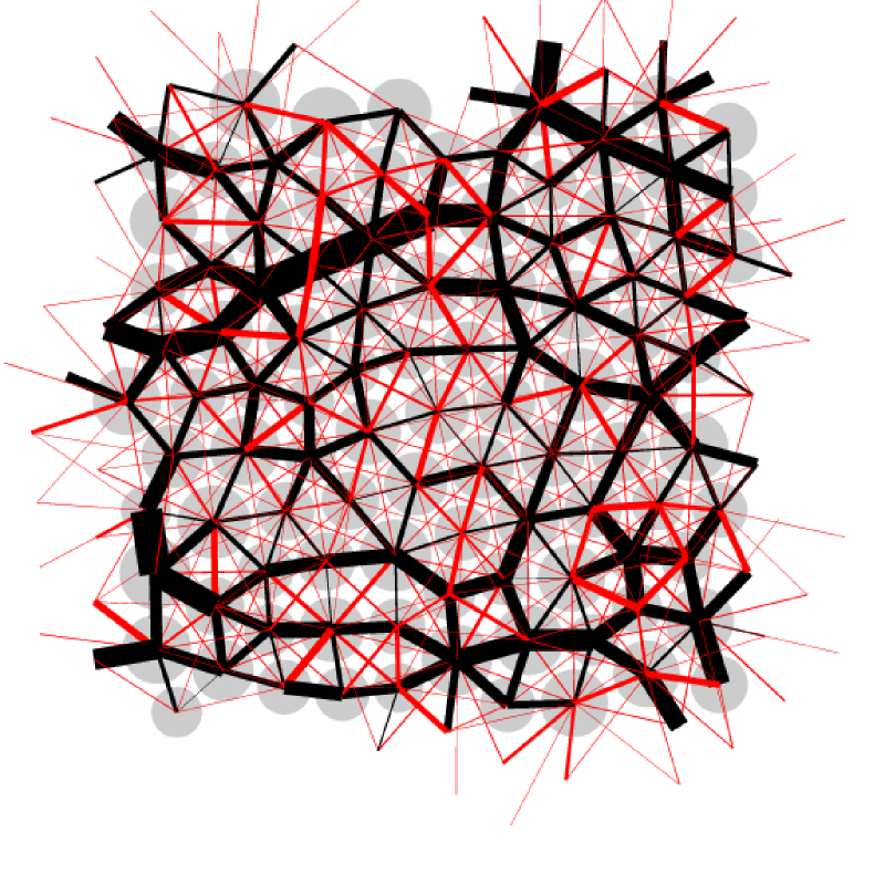
Figure 2: Snapshot of a small subvolume of linear length $10$ containing about $100$ verticies of the elastic network considered in this work assuming Eq. (38). The total periodic box of linear length $L\approx 102.3$ contains $N=10^{4}$ verticies and $9956$ harmonic springs. The light grey circles indicate the positions and diameters of the quenched polydisperse LJ bead system which was used for the construction of the elastic network as described in Sec. IV. The lines represent the quenched forces of the athermal ($T=0$) reference configuration. The dark (black) lines indicate repulsive forces between the verticies, while the light (red) lines represent tensile forces. The line width is proportional to the tension/repulsion.

III Model and algorithmic details

Hamiltonian.

To illustrate our key relations we present in Sec. V numerical data obtained using a periodic two-dimensional ($d=2$) network of harmonic springs. The model Hamiltonian is given by the sum $\hat{\cal H}=\hat{\cal H}_{\mathrm{id}}+\hat{\cal H}_{\mathrm{ex}}$ of a kinetic energy contribution $\hat{\cal H}_{\mathrm{id}}=m\sum_{i}\underline{v}_{i}^{2}/2$ (assuming a monodisperse mass $m$) and an excess potential

$$\hat{\cal H}_{\mathrm{ex}}=\sum_{l}u_{l}(r_{l})\mbox{ with }u_{l}(r)=\frac{1}{2}K_{l}\left(r-R_{l}\right)^{2}$$ (38)

where $K_{l}$ denotes the spring constant, $R_{l}$ the reference length and $r_{l}=|\underline{r}_{i}-\underline{r}_{j}|$ the length of spring $l$. The sum runs over all springs $l$ connecting pairs of beads $i$ and $j$ at positions $\underline{r}_{i}$ and $\underline{r}_{j}$. A small subvolume of the network considered is represented in Fig. 2. An experimentally relevant example for such a permanent network is provided by endlinked or vulcanized polymer networks Rubinstein and Colby (2003); Duering et al. (1991, 1994). Since the network topology is by construction permanently fixed, the shear response $G(t)$ must become finite for $t\to\infty$ for all temperatures at variance to systems with plastic rearrangements as considered, e.g., in Ref. Sausset et al. (2010). Note that the particle mass $m$ and Boltzmann’s constant $k_{\rm B}$ are set to unity. Lennard-Jones (LJ) units Allen and Tildesley (1994) are assumed throughout this paper.

Computational methods, parameters and observables.

The construction and the characterization of the reference network at zero temperature is presented in Sec. IV. As discussed in Sec. V, this network is then investigated numerically by means of standard molecular dynamics (MD) simulation Allen and Tildesley (1994); Frenkel and Smit (2002) at constant particle number $N=10^{4}$, box volume $V\approx 102.3^{2}$ and a small, but finite mean temperature $T=0.001$. Newton’s equations are integrated using a velocity-Verlet algorithm with a tiny time step $\delta t_{\mathrm{MD}}=10^{-4}$. The temperature $T$ is fixed using a Langevin thermostat with a friction constant $\zeta$ ranging from $\zeta=0.01$ up to $\zeta=5$ as specified below. An important property sampled in this study is the instantaneous stress tensor Allen and Tildesley (1994); foo (c)

$$\hat{\sigma}_{\alpha\beta}=-\frac{m}{V}\sum_{i=1}^{N}v_{i,\alpha}v_{i,\beta}+\frac{1}{V}\sum_{l}r_{l}u_{l}^{\prime}(r_{l})\ n_{l,\alpha}n_{l,\beta}$$ (39)

where the Greek indices $\alpha$ and $\beta$ denote the $d=2$ spatial directions $x$ and $y$, $v_{i,\alpha}$ the $\alpha$-component of the velocity of particle $i$ and $n_{l,\alpha}$ the $\alpha$-component of the normalized vector $\underline{r}_{l}$. The first term in Eq. (39) gives the ideal gas contribution, the second term corresponds to the Kirkwood excess stress for pair interactions. The trace of the stress tensor yields the instantaneous normal pressure $\hat{P}=-(\hat{\sigma}_{xx}+\hat{\sigma}_{yy})/d$, the off-diagonal elements $\hat{\sigma}_{xy}=\hat{\sigma}_{yx}$ are consistent with the shear stress $\hat{\tau}=\hat{\tau}_{\mathrm{id}}+\hat{\tau}_{\mathrm{ex}}$, Eqs. (10,12), obtained in Sec. II.1. The shear strain $\gamma$ is set to zero for the computation of the autocorrelation function $C(t)=\beta V\left(\langle\hat{\tau}(t)^{2}\rangle-\langle\hat{\tau}\rangle^{2}\right)$. A tiny step strain $\gamma\ll 1$ is imposed at $t=0$ in order to compute $G(t)$, as discussed in Sec. V.2, and a sinusoidal strain $\gamma(t)=\gamma_{0}\sin(\omega t)$ to measure directly the storage and loss moduli $G^{\prime}(\omega)$ and $G^{\prime\prime}(\omega)$ from the sine and cosine transforms of the instantaneous shear stress $\hat{\tau}(t)$, Eqs. (34,35). As already described in the first paragraph of Sec. II.1 we perform in both cases affine, canonical Goldstein et al. (2001) and (essentially) infinitessimal strain transformations of the box shape and the particle positions and momenta, Eqs. (5,6). Note that the transformation of the momenta is, however, not important for the simulations presented here where we focus on low temperatures and mainly on high values of the Langevin friction constant. Moreover, as shown in Ref. Wittmer et al. (2015), similar results, especially concerning Eq. (2), are also obtained using Brownian dynamics or Monte Carlo simulations Allen and Tildesley (1994); Frenkel and Smit (2002).

IV Reference configuration

Construction of network.

As explained in detail in Ref. Wittmer et al. (2013a), our network has been constructed using the dynamical matrix $\underline{\underline{M}}$ of a polydisperse LJ bead glass comprising $N=10^{4}$ particles. Prior to forming the network a LJ bead system has been quenched to $T=0$ using a constant quenching rate and imposing a normal pressure $P=2$. The original LJ beads are represented in Fig. 2 by grey polydisperse circles, the permanent spring network created from the quenched bead system by lines between verticies. The network has a number density $\rho\approx 0.96$ corresponding to a linear periodic box length $L\approx 102.3$. Using Eq. (39) one determines a normal pressure $P\approx 2$ and a small, but finite shear stress $\tau\approx 0.011614$ (determined to high precision for reasons given below). Using Eq. (27) one obtains the affine shear elasticity $\mu_{\mathrm{A}}\approx 34.3$. By construction the total force acting on each vertex of the reference network vanishes albeit the repulsive and tensile forces transmitted along each spring do in general not as shown in Fig. 2. Due to the periodic boundary conditions the finite residual (normal and shear) stress does not relax. Albeit being small, it is important to properly account for the finite, quenched shear stress $\tau$ of the reference for all the correlation functions considered. We also note that the force network, Fig. 2, is strongly inhomogeneous with zones of weak attractive links embedded within a strong repulsive skeleton as discussed in Refs. Wittmer et al. (2002); Tanguy et al. (2002).

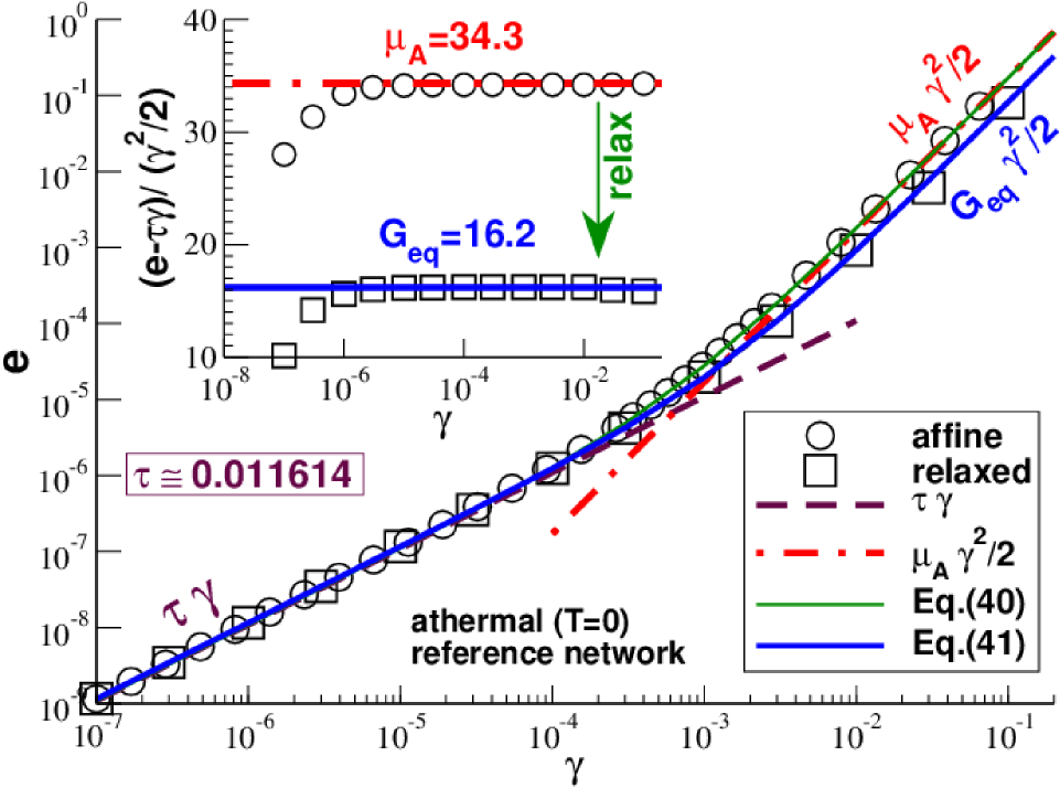
Figure 3: Energy difference per volume $e$ after an affine strain $\gamma$ is applied (circles) and after the network has relaxed to the new ground state (squares). Main panel: Double-logarithmic representation of $e$ vs. $\gamma$. The thin solid line indicates Eq. (40), the bold solid line Eq. (41). Inset: Half-logarithmic representation of reduced energy increment $(e-\tau\gamma)/(\gamma^{2}/2)$ vs. $\gamma$ where the residual shear stress $\tau=0.011614$ has been taken off. The shear modulus $G_{\mathrm{eq}}\approx 16.2$ is obtained from the rescaled groundstate energy (squares).

Affine displacements.

As shown in Fig. 3, it is possible to obtain numerically the shear stress $\tau$ and the affine shear elasticity $\mu_{\mathrm{A}}$ from the energy increment per volume $e\equiv(\hat{\cal H}_{\mathrm{ex}}(\gamma)-\hat{\cal H}_{\mathrm{ex}}(0))/V$ caused by an affine shear strain $\gamma$ (spheres). In agreement with Eq. (7), the energy increases as

$$e=\tau\gamma+\mu_{\mathrm{A}}\gamma^{2}/2$$ (40)

as shown by the thin solid line in the main panel of Fig. 3. The asymptotic limits for small and large $\gamma$ are indicated by, respectively, the dashed line and the dash-dotted line. We have used for the coefficients $\tau$ and $\mu_{\mathrm{A}}$ in Eq. (40) the values obtained using Eq. (12) and Eq. (13). This is merely a self-consistency check since both properties are actually defined assuming a virtual affine strain transformation as reminded in Sec. II.1 Wittmer et al. (2013a); Doi and Edwards (1986). As shown in the inset, an accurate verification of $\mu_{\mathrm{A}}$ over essentially the full $\gamma$-range is obtained by plotting in half-logarithmic coordinates the reduced energy $(e-\tau\gamma)/(\gamma^{2}/2)$. For the smallest $\gamma$ an even more precise value of the substracted residual shear stress $\tau$ is required to collapse even these data points on the dash-dotted horizontal line.

Figure 4: Snapshot of non-affine displacement field after an affine shear strain with $\gamma=0.01$ is applied and the system is allowed to relax. The arrow length is proportionel to the non-affine particle displacements. The displacement field is correlated over distances much larger than the typical particle distance. All displacements are strictly linear in $\gamma$.

Non-affine displacements.

The forces $\underline{f}_{i}$ acting on the verticies $i$ of an affinely strained network do not vanish in general. Following Ref. Tanguy et al. (2002) the network is first relaxed by steepest descend, i.e. imposing displacements proportional to the force, and then by means of the conjugate gradient method Thijssen (1999). These non-affine displacements lower the final energy of the strained system as indicated by the squares in Fig. 3. As shown by the bold solid line in the main panel, these final energies scale as

$$e=\tau\gamma+G_{\mathrm{eq}}\gamma^{2}/2.$$ (41)

This scaling is similar to the affine strain energy, Eq. (40), having the same linear term but with $\mu_{\mathrm{A}}$ being replaced by the shear modulus $G_{\mathrm{eq}}$. As shown in the inset, these energies can thus be used to determine $G_{\mathrm{eq}}\approx 16.2$ by taking again into account the quenched shear stress at $\gamma=0$. It follows from Eq. (40) and Eq. (41) that due to the non-affine displacements a substantial fraction $1-G_{\mathrm{eq}}/\mu_{\mathrm{A}}\approx 1/2$ of the affine strain energy is relaxed for large $\gamma$ in agreement with Ref. Tanguy et al. (2002). A snapshot of these non-affine displacements is given in Fig. 4. Note that the non-affine displacements are correlated over distances much larger than the typical particle distance and one thus expects deviations from standard continuum mechanics if similar length scales are probed.

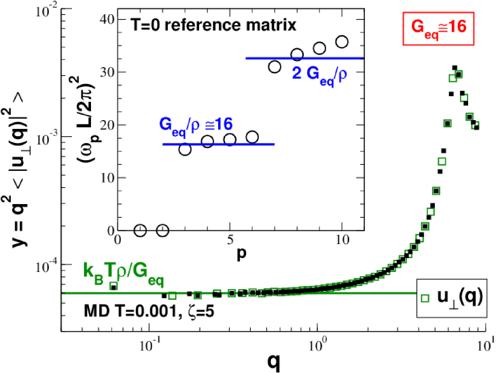
Figure 5: Determination of shear modulus $G_{\mathrm{eq}}$. Inset: Lowest eigenfrequencies $\omega_{p}$ obtained by diagonalization of the dynamical matrix. The bold horizontal lines correspond to $G_{\mathrm{eq}}/\rho\approx 16$ according to Eq. (43) fitting the eigenvalues for $p=3,4,5,6$. Main panel: Fourier transformed transverse displacement field for a temperature $T=0.001$ as a function of wavevector $q$. The horizontal line corresponds again to $G_{\mathrm{eq}}\approx 16$. The open symbols indicate data obtained using the ground state positions as reference, the filled symbols assume the average vertex position as reference.

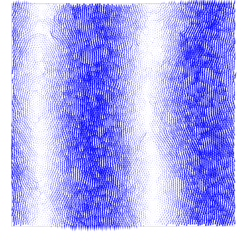
Figure 6: Eigenvector for $p=4$ ($n=1,m=0$) corresponding to a transverse planewave with wavector $\underline{q}$ pointing in the horizontal direction, i.e. with displacements essentially in the vertical direction, and wavelength $\lambda=L$. Interestingly, heterogeneous deviations from the planewave solution of continuum mechanics are even visible for this low eigenmode.

Eigenstates of the reference.

Following Refs. Wittmer et al. (2002); Tanguy et al. (2002) the shear modulus $G_{\mathrm{eq}}$ of the network at $T=0$ may alternatively be computed from the lowest non-trivial eigenfrequencies $\omega_{p}$. (The running index $p$ increases with frequency.) This is shown in the inset of Fig. 5. The eigenfrequencies $\omega_{p}^{2}$ have been determined by diagonalization of the dynamical matrix $\underline{\underline{M}}$ by means of Lanczos’ method Thijssen (1999). It follows from continuum elasticity Landau and Lifshitz (1959) that the eigenfunctions must be planewaves with wavevectors $\underline{q}$ quantified by the boundary conditions, i.e. $(q_{x},q_{y})=(2\pi/L)\ (n,m)$ with $n,m=0,\pm 1,\ldots$ being two quantum numbers. An example for such a planewave is given in Fig. 6 for $p=4$ and the pair of quantum numbers $(n,m)=(1,0)$. For the wavelength this implies

$$\lambda_{p}=2\pi/|\underline{q}|=L/\sqrt{n^{2}+m^{2}}$$ (42)

and for the eigenfrequencies of the transverse modes

$$\omega_{p}=\frac{2\pi c_{\bot}}{L}\sqrt{n^{2}+m^{2}}\mbox{ with }c_{\bot}=\sqrt{G_{\mathrm{eq}}/\rho}$$ (43)

being the transverse wavevelocity. As shown by the horizontal lines, we obtain by fitting Eq. (43) to the frequencies for $p=3,4,5,6$ (corresponding to $n^{2}+m^{2}=1$) that $G_{\mathrm{eq}}\approx 16$ and $c_{\bot}\approx 4$. Interestingly, the degeneracy of the eigenvalues expected from continuity elasticity is already lifted for $p=7,8,9,10$ ($n^{2}+m^{2}=2$), i.e. the box size $L$ does not allow a precise determination of $G_{\mathrm{eq}}$ using these eigenvalues. Deviations from the planewave solution are even visible from the eigenvector for $p=4$ presented in Fig. 6. Continuum elasticity must break down in any case if wavelengths of order of about the particle distance are probed, $\lambda\approx 1$. This implies that Eq. (43) can at best hold up to a frequency $\omega=2\pi c_{\bot}/\lambda\approx 25$. We come back to this issue in Sec. V.1 and Sec. V.3.

V Finite-temperature computational results

V.1 Some static properties

Introduction.

Since the temperature $T=0.001$ is rather small, one expects all static properties such as the pressure $P$ or the elastic modulus $G_{\mathrm{eq}}$ to be similar to their ground state values. As we have checked comparing various methods one confirms indeed that $P\approx P_{\mathrm{ex}}\approx 2$, $\tau\approx\tau_{\mathrm{ex}}\approx 0.011$, $\mu_{\mathrm{A}}\approx\mu_{\mathrm{A,ex}}\approx 34$, $\sigma_{\mathrm{F}}\approx\sigma_{\mathrm{F,ex}}\approx 18$ and $G_{\mathrm{eq}}\approx 16$. The same applies in fact to all small temperatures $T\ll 1$.

Displacement correlations.

A finite-$T$ method for computing $G_{\mathrm{eq}}$, which is also of experimental relevance Klix et al. (2012), is presented in the main panel of Fig. 5. Using an ensemble of $10^{4}$ configurations sampled over a total time interval $10^{6}$ with $\zeta=5$ we obtain first the displacements $\underline{u}_{i}$ for each vertex particle $i$ of the network either by taking the position of the ground state network as reference for defining the displacement (open squares) or alternatively the average particle position in the ensemble (filled squares). The displacement field $\underline{u}(\underline{r})=\sum_{i}\underline{u}_{i}\delta(\underline{r}-\underline{r}_{i})$ is then Fourier transformed according to $\underline{u}(\underline{q})=\sum_{i=1}^{N}\exp(i\underline{q}\cdot\underline{r})\ \underline{u}(\underline{r})/\sqrt{N}$ Klix et al. (2012). Note that the wavevector $\underline{q}$ must be commensurate to the square simulation box of linear length $L$, Eq. (42). The component of $\underline{u}(\underline{q})$ perpendicular to $\underline{q}$ corresponds to the transverse component $\underline{u}_{\bot}(\underline{q})$ of the Fourier transformed displacement field. Using that according to the equipartition theorem every independent elastic mode corresponds to an average kinetic or potential energy $\mbox{$k_{\rm B}T$}/2$, continuum mechanics implies that Landau and Lifshitz (1959); Klix et al. (2012)

$$y\equiv q^{2}\left<|\underline{u}_{\bot}(\underline{q})|^{2}\right>\to\mbox{$k_{\rm B}T$}\rho/G_{\mathrm{eq}}\ \mbox{ for }q\to 0$$ (44)

where the average $\langle\ldots\rangle$ is taken over the ensemble of stored configurations. As can be seen from Fig. 5, $y$ becomes rapidly constant below $q\approx 1$ confirming $G_{\mathrm{eq}}\approx 16$ as indicated by the bold horizontal line. Incidentally, both definitions of the displacement field yield identical results. Since only the second definition using the average particle position can normally be used in experimental studies, this is rather reassuring. Note also that the first peak for large wavevectors corresponds to a wavelength $\lambda=2\pi/q\approx 1$ of order of the typical particle distance where continuum mechanics should break down.

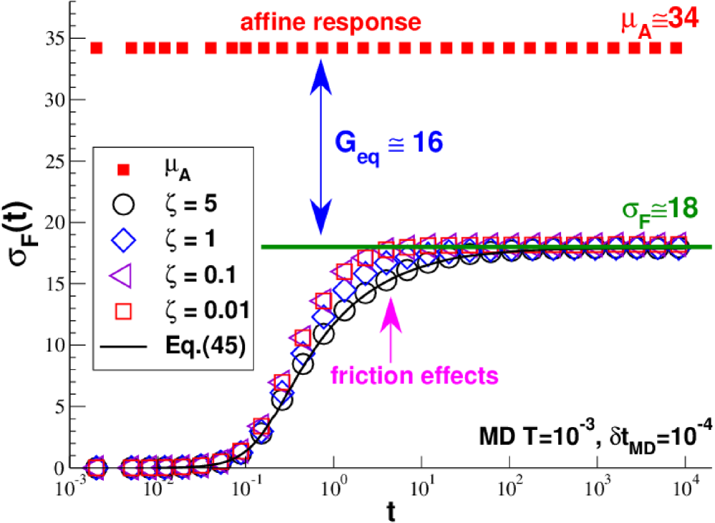
Figure 7: Determination of $G_{\mathrm{eq}}\approx 16$ using Eq. (22) as a function of the sampling time $t$ at $T=0.001$. While the simple average $\mu_{\mathrm{A}}\approx 34$ converges immediately (small filled squares), the stress fluctuations $\sigma_{\mathrm{F}}(t)$ are seen to increase monotonously to the large-$t$ limit $\sigma_{\mathrm{F}}\approx 18$ (bold solid line). This is shown for four different friction constants $\zeta=5,1,0.1$ and $0.01$. The thin solid line compares the data for $\zeta=5$ with the integrated correlation function $C(t)$ using Eq. (45).

Stress fluctuations.

While it is thus possible to get $G_{\mathrm{eq}}$ from the displacement correlations, it is from the computational point of view more convenient to determine the modulus using the stress-fluctuation formula, Eq. (22). This is shown in Fig. 7 where the affine shear elasticity $\mu_{\mathrm{A}}$ (small filled squares) and the stress-fluctuation term $\sigma_{\mathrm{F}}(t)$ are presented as functions of the sampling time $t$. (The notation $\sigma_{\mathrm{F}}$ without time argument refers to the static thermodynamic large-$t$ limit, while $\sigma_{\mathrm{F}}(t)$ indicates that this property has been determined using a finite time window $t$.) While the simple average $\mu_{\mathrm{A}}$ is obtained immediately, $\sigma_{\mathrm{F}}(t)$ is seen to increase monotonously from zero to the large-$t$ plateau $\sigma_{\mathrm{F}}\approx 18$ (horizontal bold solid line). Friction effects are important only in the intermediate sampling time window between $t\approx 0.1$ and $10$ where the stress fluctuations strongly increase. The data obtained for Langevin friction constants $\zeta=0.1$ and $0.01$ are essentially identical. The time dependence of $\sigma_{\mathrm{F}}(t)$ for different friction constants is further analysed at the end of Sec. V.2.

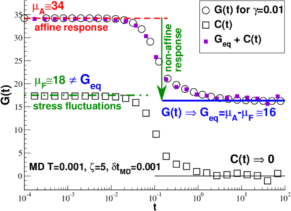
Figure 8: Stress relaxation modulus $G(t)$ and autocorrelation function $C(t)$ sampled by means of a Langevin thermostat of friction constant $\zeta=5$. An affine step strain $\gamma=0.01$ is applied at $t=0$ to determine $G(t)$.

V.2 Time domain of key relations

High friction limit.

We turn now to the numerical verification of the key relations stated in the Introduction focusing first on results obtained in the time domain which have already been reported in Ref. Wittmer et al. (2015). The data presented in Fig. 8 have been computed using a Langevin thermostat with one high friction constant $\zeta=5$. This is done merely for presentational reasons since in this limit the kinetic degrees of freedom can be disregarded and oscillations are suppressed. The stress relaxation modulus $G(t)$ given has been computed as indicated in panel (b) of Fig. 1 by applying an affine canonical shear strain $\gamma=0.01$ and by averaging over 1000 runs starting from independent configurations at $t=0^{-}$. Due to the strong damping $G(t)$ decreases monotonously from $G(0^{+})=\mu_{\mathrm{A}}$ to $G_{\mathrm{eq}}$ while $C(t)$ decays from $C(0)=\sigma_{\mathrm{F}}$ to zero. Confirming Eq. (2), only after vertically shifting $C(t)\rightarrow C(t)+G_{\mathrm{eq}}$ one obtains a collapse on the directly computed modulus $G(t)$. This is the most important numerical result of the present work.

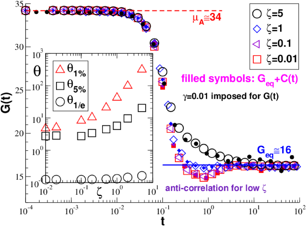
Figure 9: Stress relaxation modulus $G(t)$ obtained using a step strain (open symbols) and the rescaled autocorrelation function $G_{\mathrm{eq}}+C(t)$ at $\gamma=0$ (filled symbols) for several friction constants $\zeta$. Inset: Shear stress relaxation time $\theta(\zeta)$ measured using $\theta_{1/e}$, $\theta_{5\%}$ and $\theta_{1\%}$ defined in the main text.

Friction effects and stress relaxation time.

A similar scaling collapse of $G(t)$ and $C(t)+G_{\mathrm{eq}}$ has been also obtained for different friction constants $\zeta$ as may be seen from Fig. 9. As one expects, the MD data decays more rapidly with decreasing $\zeta$ and reveals anti-correlations for the lowest $\zeta$ probed. The effect of the friction constant may be compactly described using the stress relaxation time $\theta$ shown in the inset of Fig. 9. We compare here three different definitions. The definition $C(t=\theta_{1/e})=\sigma_{\mathrm{F}}/e$, indicated by spheres, describes the time where the correlation functions first becomes small. This simple definition underestimates correlations at larger times. Alternatively, one may attempt to define $\theta$ by the ratio $c_{1}/c_{0}$ of the first to the zeroth moment of $C(t)$ with $c_{n}\equiv\int_{0}^{\infty}t^{n}C(t)\text{d}t$ (not shown). Unfortunately, $c_{1}$ is found to converge badly and we have not been able to obtain reliable values over the full $\zeta$-range. A numerically well-behaved alternative is based on an exact relation between the autocorrelation function $C(t)$ and the monotoneously increasing fluctuation term $\sigma_{\mathrm{F}}(t)$ determined as a function of the sampling time $t$. Assuming time-translational invariance it can be shown Wittmer et al. (2015) that

$$y(t)\equiv 1-\frac{\sigma_{\mathrm{F}}(t)}{\sigma_{\mathrm{F}}}=\frac{2}{t}\int_{0}^{t}\text{d}s\ (1-s/t)\ \frac{C(s)}{\sigma_{\mathrm{F}}},$$ (45)

i.e. the dimensionless ratio $y(t)$ characterizes the difference of the zeroth and the first moment of the autocorrelation function integrated up to $t$. That this relation holds can be seen from the thin line presented in Fig. 7. We note en passant that $y(t)$ must ultimately vanish slowly as $1/t$ since the integral over $C(s)$ in Eq. (45) becomes constant Wittmer et al. (2015). (This $1/t$-decay is consistent with the general finite-sampling time corrections for fluctuations Landau and Binder (2000).) Since $\sigma_{\mathrm{F}}(t)$ can be determined directly, one may define $\theta(\zeta)$ using a fixed ratio $y(\theta)$. We have presented in Fig. 9 the constants $y(\theta_{5\%})=5\%$ (squares) and $y(\theta_{1\%})=1\%$ (triangles). Note that $\theta_{5\%}$ corresponds to the time where $\sigma_{\mathrm{F}}(t)$ begins to saturate, while $\theta_{1\%}$ indicates the time where the stress-correlations become neglible and $\sigma_{\mathrm{F}}(t)$ thus allows a good estimation of $G_{\mathrm{eq}}$ using the stress-fluctuation formula.

V.3 Oscillatory shear

Direct determination of $G^{\prime}(\omega)$ and $G^{\prime\prime}(\omega)$.

As already stressed in Sec. II.3, the relaxation modulus $G(t)$ is commonly determined experimentally by inverse Fourier transformation of the storage modulus $G^{\prime}(\omega)$ and/or the loss modulus $G^{\prime\prime}(\omega)$ obtained in a linear viscoelastic measurement imposing an oscillatory shear Witten and Pincus (2004); Rubinstein and Colby (2003). Motivated by this we perform non-equilibrium MD simulations in the linear response limit by imposing a sinusoidal shear strain of frequency $\omega$ with an amplitude $\gamma_{0}=0.001$. (By varying $\gamma_{0}$ it has been checked that all reported values are in the linear regime.) This is done by performing every time step $\delta t_{\mathrm{MD}}=10^{-4}$ an affine canonical strain, Sec. II.1. We use production runs of total length $pT_{\mathrm{\omega}}$ with $T_{\mathrm{\omega}}=2\pi/\omega$ and at least $p=100$ oscillation periods, i.e. the computational load increases as $p/\omega$ with decreasing frequency. This sets a lower limit $\omega\approx 10^{-3}$ for the angular frequencies we have been able to sample. Two production runs are compared to rule out transient behavior. The instantaneous shear stress $\hat{\tau}(t)$ is sampled each $\delta t_{\mathrm{MD}}$. Using Eq. (34) and Eq. (35) one obtains $G^{\prime}(\omega)$ and $G^{\prime\prime}(\omega)$ as indicated by open triangles in Fig. 10, where we focus for simplicity on one value $\zeta=5$ of the friction constant, and large open symbols in Fig. 11, where data for different $\zeta$ are presented.

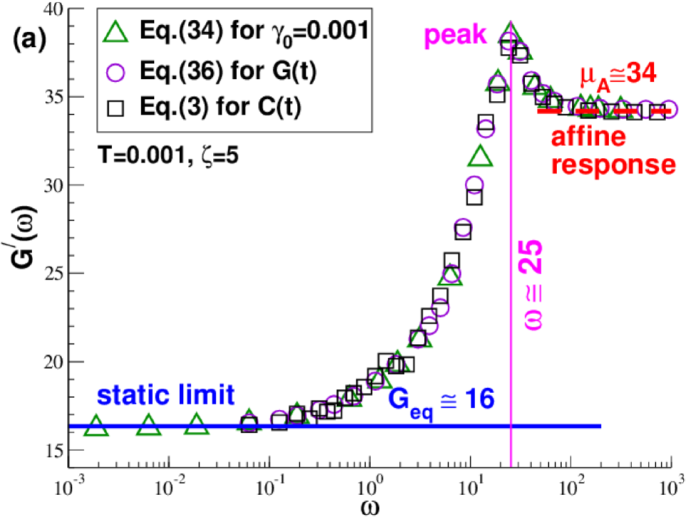
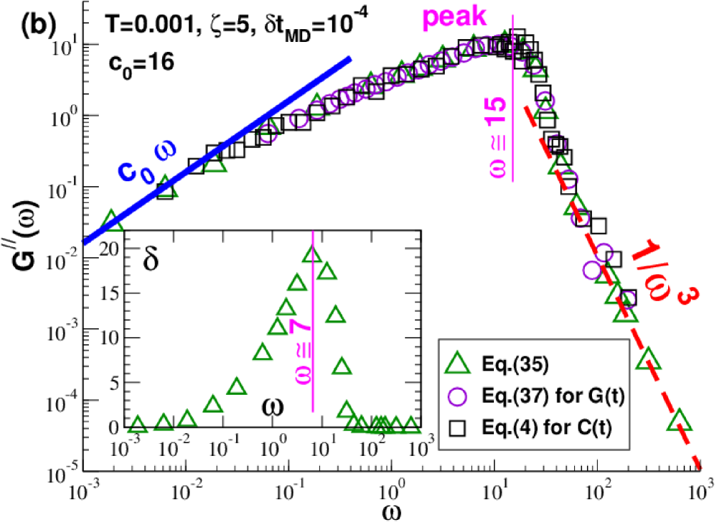
Figure 10: Oscillatory shear moduli (a) $G^{\prime}(\omega)$ using a log-linear representation and (b) $G^{\prime\prime}(\omega)$ using a double-logarithmic representation for a large friction constant $\zeta=5$. We compare the Fourier coefficients (triangles) obtained by applying a sinusoidal shear strain with amplitude $\gamma_{0}=0.001$ to the Fourier transformed step-strain relaxation modulus $G(t)$ (circles) and shear autocorrelation function $C(t)$ (squares). The bold solid lines indicate the expected asymptotic limits for small $\omega$, the dashed lines the large-$\omega$ asymptotics, the thin vertical lines the frequencies $\omega\approx 25$ and $\omega\approx 15$ of the maxima of both moduli. The latter values coincide with the breakdown of continuum elasticity at a planewave frequency $\omega=2\pi c_{\bot}/\lambda$ with $\lambda\approx 1$ probing the typical particle distance. Inset of (b): Phase angle $\delta$ with maximum $\delta\approx 20^{0}$ at $\omega\approx 7$ (vertical line).

Test of key relations.

These values of $G^{\prime}(\omega)$ and $G^{\prime\prime}(\omega)$ are compared in Fig. 10 with the Sine-Fourier and Cosine-Fourier transforms of the shear modulus $G(t)$ obtained from the step strain experiment (circles) and of the shear stress autocorrelation function $C(t)$. To reduce the well-known (but considering our tiny time step $\delta t_{\mathrm{MD}}$ surprisingly severe) numerical problems at large frequencies ($\omega\gg 10$), Filon’s quadrature method Allen and Tildesley (1994) is used for the Fourier integration. These Fourier transforms collapse nicely on the respective directly computed moduli $G^{\prime}(\omega)$ and $G^{\prime\prime}(\omega)$. The crucial point is here that it is $G_{\mathrm{eq}}+C^{\prime}(\omega)$ which collapses on $G^{\prime}(\omega)$, while $C^{\prime}(\omega)$ does not being much too small considering that $G_{\mathrm{eq}}\approx 16$, as seen in panel (a). We have verified that a similar data collapse for $G_{\mathrm{eq}}+C^{\prime}(\omega)$ onto $G^{\prime}(\omega)$ and $C^{\prime\prime}(\omega)$ onto $G^{\prime\prime}(\omega)$ is also obtained for other friction constants as may be seen from Fig. 11. Having settled this fundamental scaling issue let us turn finally to the description of the general shape and asymptotic behavior of both moduli.

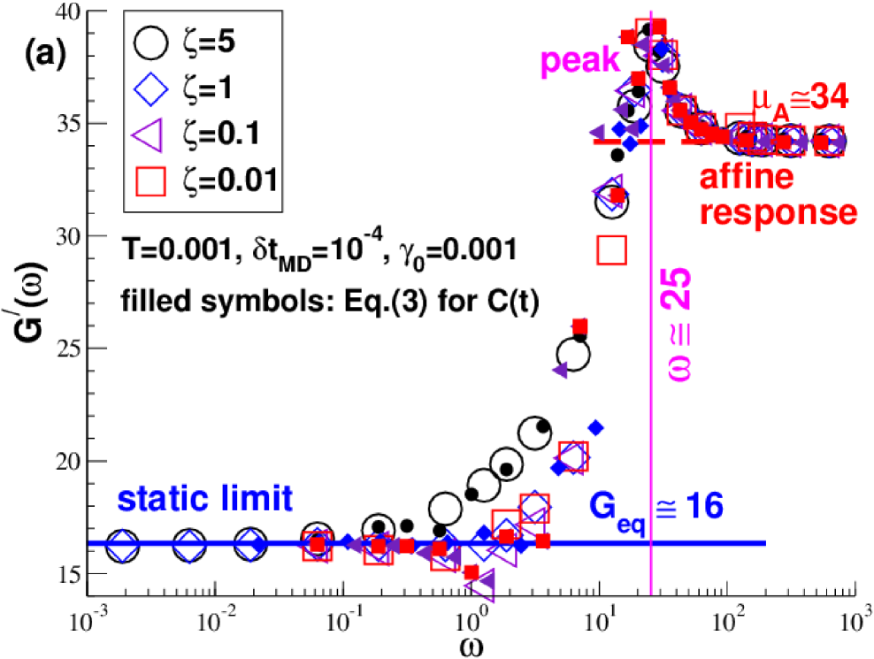
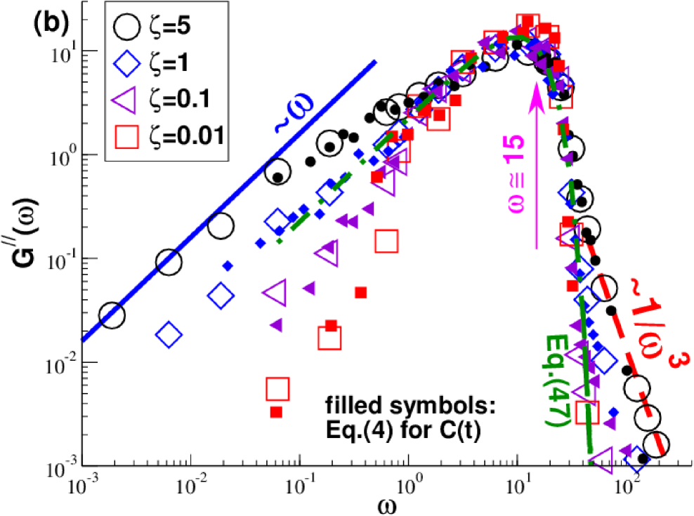
Figure 11: Effect of Langevin friction constant $\zeta$ with open symbols referring to data obtained using oscillatory shear with amplitude $\gamma_{0}=0.001$: (a) Storage modulus $G^{\prime}(\omega)$. The friction constant $\zeta$ only matters in an intermediate frequency range between $\omega\approx 0.1$ and $\omega\approx 10$ below the peak at $\omega\approx 25$. (b) Loss modulus $G^{\prime\prime}(\omega)$. The dot-dashed line is a phenomenological fit for large $\omega$ and small $\zeta$ assuming Eq. (47).

Low-frequency limit.

The low-$\omega$ limit of $G^{\prime}(\omega)$ and $G^{\prime\prime}(\omega)$ are readily obtained by expanding $\sin(x)$ in Eq. (3) and $\cos(x)$ in Eq. (4). As one expects Rubinstein and Colby (2003), one obtains to leading order that $G^{\prime}(\omega)\to G_{\mathrm{eq}}$, Eq. (1), and $G^{\prime\prime}(\omega)\to\omega c_{0}$ as indicated by bold solid lines in Fig. 10 and Fig. 11. We have fitted $G^{\prime\prime}(\omega)$ for $\zeta=5$ using the independently determined value $c_{0}\approx 16$.

Intermediate peaks.

In the intermediate frequency regime one observes a striking peak at $\omega\approx 25$ for $G^{\prime}(\omega)$, i.e. at the planewave frequency corresponding to the typical particle distance, Eq. (43), and at a slightly smaller value $\omega\approx 15$ for $G^{\prime\prime}(\omega)$. The phase angle $\delta$ characterizing the ratio $G^{\prime\prime}(\omega)/G^{\prime}(\omega)\equiv\tan(\delta)$ is presented in the inset (in grad). It reveals a maximum at $\omega\approx 7$.

High-frequency limit.

In the high-frequency limit it becomes increasing difficult to relax the imposed affine strain by non-affine displacements and, hence, to dissipate the work done on the system. This implies that

$$G^{\prime}(\omega)=G_{\mathrm{eq}}+C^{\prime}(\omega)\to(\mu_{\mathrm{A}}-\sigma_{\mathrm{F}})+\sigma_{\mathrm{F}}=\mu_{\mathrm{A}}$$ (46)

for $\omega\to\infty$ (bold dashed horizontal lines), while $G^{\prime\prime}(\omega)$ decays with a non-universal (see below) sharp cutoff (dashed and dash-dotted lines). This asymptotic behavior can be also understood on mathematical grounds by expanding Eq. (3) and Eq. (4) by integration by parts. This leads to two series-expansions in terms of even and odd derivatives of $C(t)$ taken at $t=0$ for, respectively, $G^{\prime}(\omega)$ and $G^{\prime\prime}(\omega)$. We remind that $C(t)$ is an even function for classical systems Allen and Tildesley (1994); Hansen and McDonald (2006) and that in a MD simulation $C(t)$ must become analytic at sufficiently short times ($\delta t_{\mathrm{MD}}<t\ll 1/\zeta$) where thermostat effects are negligible. (Strict non-analyticity of $C(t)$ at $t=0$ is formally found, e.g., for the Maxwell model or the polymer Rouse model Doi and Edwards (1986).) Analyticity at $t=0$ implies that the (converging) expansion of $G^{\prime}(\omega)$ is dominated by its first term for $\omega\to\infty$. This demonstrates Eq. (46). The effective odd derivatives of $C(t)$ must, however, become negligible with decreasing friction $\zeta$, increasing angular frequency $\omega$ and decreasing time step $\delta t_{\mathrm{MD}}$. Hence, $G^{\prime\prime}(\omega)$ must rapidly vanish. This point is further investigated in the final paragraph of this section.

Friction effects.

The friction effects presented in Fig. 11 are rather small for $G^{\prime}(\omega)$ due to the large static constants $G_{\mathrm{eq}}$ and $\mu_{\mathrm{A}}$ dominating the storage modulus. As one would expect, they are more marked for the loss modulus $G^{\prime\prime}(\omega)$, especially at low frequencies where the thermostat has more time to dissipate the applied mechanical energy, but also at the large-$\omega$ cutoff. For $\zeta=5$ one might be tempted to fit an $1/\omega^{3}$-decay (dashed lines) which indicates an effective non-analytical behavior of $C(t)$ at short times. With decreasing $\zeta$ the loss modulus is, however, better described by the exponential decay

$$G^{\prime\prime}(\omega)=\sigma_{\mathrm{F}}\sqrt{\pi/4}\ x\ \exp(-x^{2}/2)\mbox{ with }x=\omega\tilde{\theta}$$ (47)

as indicated by the dash-dotted line in panel (b) of Fig. 11. This phenomenological fit is the Cosine-Fourier transform assuming a Gaussian $C(t)=\sigma_{\mathrm{F}}\exp(-(t/\tilde{\theta})^{2}/2)$ with the parameter $\tilde{\theta}\approx 0.1$ determined from the short-time (high-frequency) limit. A similar phenomenological fit for the large-$\omega$ behavior of is also obtained by assuming a Lorentzian $C(t)=\sigma_{\mathrm{F}}/(1+(t/\tilde{\theta})^{2})$. We note finally that if smaller time steps and larger frequencies could be computed, one expects even for higher friction constants a similar non-algebraic cutoff, albeit with a different parameter $\tilde{\theta}(\zeta)$.

VI Conclusion

Summary.

We have studied in the present work simple isotropic solids formed by permanent spring networks. Some relevant static properties have been reviewed and characterized in Secs. II.1, IV and V.1. More importantly, we have reconsidered theoretically (Sec. II) and numerically (Sec. V) the linear-response relation between the shear stress relaxation modulus $G(t)$ and the shear stress autocorrelation function $C(t)$ both in the time (Sec. V.2, Figs. 8-9) and the frequency domain (Sec. V.3, Figs. 10 and 11). According to our key relations, Eqs. (2-4), $G(t)$ and $C(t)$ must become different in the solid limit ($G_{\mathrm{eq}}>0$) and it is thus impossible to determine $G_{\mathrm{eq}}$ from $C(t)$ or its Fourier transforms $C^{\prime}(\omega)$ and $C^{\prime\prime}(\omega)$. The short-time behavior of $C(t)$ and the large-$\omega$ limit of $C^{\prime}(\omega)$ only yield the stress-fluctuation contribution $\sigma_{\mathrm{F}}$ to the equilibrium modulus $G_{\mathrm{eq}}=\mu_{\mathrm{A}}-\sigma_{\mathrm{F}}$ (Sec. II.1) as already stressed elsewhere Yoshino and Mézard (2010); Wittmer et al. (2015). The peak frequencies observed for $G^{\prime}(\omega)$ and $G^{\prime\prime}(\omega)$ (Figs. 10 and 11) are qualitatively expected Wittmer et al. (2002); Tanguy et al. (2002) from the breakdown of continuum mechanics for large wavevectors $q\gg 1$ seen from the Fourier transformed transverse displacement field (Fig. 5).

Discussion.

It is obviously common and may often be helpful to describe a plateau of $C(t)$ at short or intermediate times (or equivalently at large or intermediate frequencies for $C^{\prime}(\omega)$) in terms of a finite shear modulus $G_{\mathrm{M}}$ of a dynamical relaxation model, such as the Maxwell model for viscoelastic fluids or the reptation model of entangled polymer melts Rubinstein and Colby (2003); Doi and Edwards (1986). However, such a model allowing the theoretical interpretation of the data should not be confused with the proper measurement procedure, Eq. (1), and a finite model parameter $G_{\mathrm{M}}$ not with the equilibrium modulus $G_{\mathrm{eq}}$ of the system which, incidentally, vanishes both for a Maxwell fluid or a linear polymer melt. In this sense different operational “static” and “dynamical” definitions of the shear modulus are used in the literature for describing glass-forming liquids close to the glass transition Klix et al. (2012); Szamel and Flenner (2011); Yoshino (2012); Yoshino and Mézard (2010); Zaccone and Terentjev (2013). This may explain why qualitatively different temperature dependences — cusp singularity Yoshino and Mézard (2010); Zaccone and Terentjev (2013) vs. finite jump Götze (2009); Klix et al. (2012); Szamel and Flenner (2011) — have been predicted recently. Hence, while our recent attempts to determine $G_{\mathrm{eq}}(T)$ for two glass-forming model systems Wittmer et al. (2013a) are consistent with a continuous cusp, this is not necessarily in contradiction with a jump singularity for $G_{\mathrm{M}}(T)$ determined from an intermediate shoulder of $C(t)$ Klix et al. (2012); Flenner and Szamel (2015).

Outlook.

We note finally that generalizing our key relations one obtains readily that

$$M(t)=C(t)+M_{\mathrm{eq}}\ \mbox{ for }t>0$$ (48)

for the relaxation modulus $M(t)$ of any continuous intensive variable $I$ with $M_{\mathrm{eq}}=\partial I/\partial X$ being the equilibrium modulus and $C(t)=\beta V\langle\delta\hat{I}(t)\delta\hat{I}(0)\rangle$ the corresponding autocorrelation function computed at a constraint thermodynamically conjugated extensive variable $X$. In the frequency domain this leads to $M^{\prime}(\omega)=M_{\mathrm{eq}}+C^{\prime}(\omega)$ and $M^{\prime\prime}(\omega)=C^{\prime\prime}(\omega)$. A natural example is provided by the relaxation modulus $M(t)=K(t)$ associated to the normal pressure $I=P$. While $C(t)$ and $C^{\prime}(\omega)$ must obviously vanish in the static limit for, respectively, large times and small frequencies, $K(t)$ and $K^{\prime}(\omega)$ approach a finite compression modulus $M_{\mathrm{eq}}=K_{\mathrm{eq}}$ for stable (non-critical) thermodynamic systems.